Use of Active RFID and Environment-Embedded Sensors for Indoor Object Location Estimation 9
Sink
Fridge
Cabinet
Door
ShoesBox
KitchenCabinet
Bed
Table
Sofa
Shelf
StereoShelf
DeskCabinet
Desk
TVShelf
X
Y
O
Chair
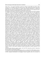
Experiment Environment
Active RFID Reader
1
2
3
4
5
6
7
8
9
10

11
12
13
Fig. 7. Supposed Object Locations and RF Readers
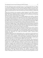
Best Accuracy
Fig. 8. Location Estimation Performance by KNN Algorithm
227
Use of Active RFID and Environment-Embedded Sensors for Indoor Object Location Estimation
10 Will-be-set-by-IN-TECH
According to Fig. 8, the pattern recognition approach works effectively in discriminating
each class from others, although there is slight dispersion in estimation performance between
different k values.
3.2 Location estimation based on object motion and human behavior
Another approach to improve object localization performance is to make the best use of
sensing information. As mentioned before, several kinds of sensors are used in our work.
Vibration sensors attached inside RFID tags are supposed to provide the system with the
information about object motion state, whereas, sensors embedded in the environment are
supposed to provide the information about human behavior and location.
It is important to perceive the moment that an object is placed for estimating its location with
sensors in the environment effectively. The vibration sensor on each RFID tag offers a great
solution to meet this requirement by detecting object motion state. However, to integrate the
vibration sensors into our system needs another problem to be solved.
Generally, active RFID tags are produced under the following policies, 1) saving the battery,
2) miniaturizing the size, and 3) cutting down the cost. To follow these policies, the frequency
of data transmission and the performance of vibration sensor inside are set up to be low.
These restrictions cause some significant problems. For example, the system cannot detect the
moment that object motion state changes in real-time because vibration sensor data requires a
moment, which is the sampling rate, to convey its reaction to the system. In addition, vibration
sensor often fails to detect object motion in the case that the movement is faint. However,
object motion detected with vibration sensor is considered as the most important information

in our system because the system uses vibration information to determine the timing to
estimate object location. To deal with the time delay between actual object movement and
vibration detection, we stagger a few seconds in our algorithm to estimate the exact moment
that an object starts to move.
The concrete location estimation algorithm based on environment-embedded sensors and
vibration sensor is constructed as follows. Our system can estimate the following three cases
individually online by combining detected reaction of each sensor. a) Object is put on and
taken away from a table. b) Object is put on and taken away from a sofa. c) Object is put into
and taken out of a drawer. That is to say, as long as the movement of object is concerned about
the area where we installed embedded sensors, we can estimate its behavior. To be concrete,
our system can detect not only the final location where object is placed, but also the state of
object in starting and quitting movement. The system estimates the two kinds of object state
as follows.
3.2.1 Estimation of movement start
In this section, we describe an algorithm to detect the start of object movement and to estimate
the original location from which object begins to move. On the occasion of estimation, we
assume that target object is in a still state before the system receives any change of sensor
state.
1. Check the state of environment-embedded sensors
According to the embedded sensors. if an object starts to move from a place where sensors
are installed, the system can detect the exact moment with the related sensors. Even if the
object moves from a place where no sensors are installed, the system can also recognize the
moment by referring to the reaction of the vibration sensor and other embedded sensors.
228
Deploying RFID – Challenges, Solutions, and Open Issues
Use of Active RFID and Environment-Embedded Sensors for Indoor Object Location Estimation 11
2. Check the state of vibration sensor
If a vibration sensor also reacts soon after the embedded sensor reaction, the system
estimates that object movement should have something to do with the sensor-embedded
place. In other words, the object is very likely to be moved from that place.

3. Recheck the state of environment-embedded sensors
After the vibration sensor reaction, if the system receives the reaction of the same
embedded sensor, it indicates that the object must be moved from the place.
To make the general rules mentioned above clearer, we pick up a typical scene to demonstrate
the estimation rules in Fig. 9. Figure 9 shows the scene that an object is moved from the table.
Firstly, the system can detect the state that something is on the table by checking the reaction
existence of the table sensor. Secondary, when the object moves, the vibration sensor reaction
will inform us of the timing of motion start. If the object does move from the table, the change
of table sensor data will indicate the strong relativity of the object and the table. Thus, the
system can estimate the object has been moved from the table in good possibility.
Table Sensor Reaction
1
if ON > ON
2
Vibration Sensor Reaction
if OFF > ON
3
Table Sensor Reaction
if ON > OFF
object is moved from the table
Estimation:
Fig. 9. Sample of Movement Start Estimation
Whereas, the process of object location estimation based on sensors is described as follows.
3.2.2 Estimation of movement end
In this process, we describe an algorithm to detect the end of object movement and to estimate
the final location where the object is placed. The system estimates the object location on the
assumption that target object has been moving until the vibration sensor reaction disappears.
1. Receive the change of state of environment-embedded sensors
If the system receives the reaction of environment-embedded sensor on the condition that
the object is in the moving state, it will suggest that the object is close to the place where the

sensor is embedded because of the presupposition that only one user is in the environment.
2. Check the change of state in vibration sensor
The phenomenon that vibration sensor’s reaction vanishes under the condition of the
embedded sensor being active indicates the high relativity between the object and the place
where the sensor is embedded.
229
Use of Active RFID and Environment-Embedded Sensors for Indoor Object Location Estimation
12 Will-be-set-by-IN-TECH
3. Recheck the state of environment-embedded sensors
The second time reaction after the vibration sensor becomes inactive allows us to
determine that the object is placed on the place.
To make the general rules mentioned above clearer, we pick up a typical scene to demonstrate
the estimation rules in Fig. 10. Figure 10 shows the scene that an object is placed in a drawer of
a cabinet. Firstly, the system will receive a reaction from the related switch sensor in addition
to the continuous reaction from the vibration sensor on the RFID tag, which means the user
opens the drawer with the object gripped in his or her hand. Soon after that, if the reaction
of the vibration sensor disappears, the possibility of the object being put into the drawer
suddenly increases. However, this does not give the confirmation because the location where
the object is placed might have no relationship with the drawer at all. Still, if the system
receives another reaction from the same switch sensor before long the vibration sensor’s
reaction vanishes, the connection between the object’s location and the drawer becomes even
deeper than ever.
1
Switch Sensor Reaction
2
Vibration Sensor Reaction
if OFF > ON
if OFF > ON
if ON > OFF
object is placed into the Cabinet

Estimation:
3
Switch Sensor Reaction
Fig. 10. Sample of Movement End Estimation
In this way, the system estimates the motion and the location of the object by combining
the information from vibration sensor and environment-embedded sensors. The concept
of the algorithm is easy to follow, but we have to overcome some difficulties to make the
estimation algorithm work well. One of the difficulties is to deal with the time delay caused
by limited sampling rate, which we used to collect sensor data. For example, an object must
have moved before the reaction of the vibration sensor and must have been placed before
the reaction disappeared from the system. We estimate the length of time delay from actual
experiments and conquer the difficulty by taking the time lag into consideration in estimating
object motion.
Another difficulty about the vibration sensor is that sometimes it does not work well. For
example, if an object is moved roughly, vibration sensor will keep reacting throughout the
movement, however, if an object is moved silently, the vibration reaction will sometimes
disappear. This means that the system should not expect continuous vibration reaction
during the object movement. Therefore, we defined a time interval to estimate the state of
object movement more accurately. If the period from the last reaction of vibration sensor is
within that interval, the system still regards the object as moving. Because the length of that
230
Deploying RFID – Challenges, Solutions, and Open Issues
Use of Active RFID and Environment-Embedded Sensors for Indoor Object Location Estimation 13
time interval depends on the way a user moves object, we decide the parameter from actual
experiments.
Although the solution mentioned above works well in estimating object motion, it also has
a problem in other aspect. That solution makes it difficult to decide the timing when an
object is moved or when an object is placed in real-time because the system has to wait
for the time interval to make the decision. It matters when we combine the reaction of a
vibration sensor with those of environment-embedded sensors to estimate where the object

is placed. According to the estimation algorithm mentioned above, the real-time detection of
the object being placed is essential in determining the final location of the object. However,
the information that object is placed will be clarified for the first time a few seconds later after
the actual point in time. Toward this problem, the system saves a series of sensor reactions
into a temporary buffer and applies the proposed estimation rules to those data after the state
of object motion fixes. The weakness of this solution is that the system cannot estimate object
location in real-time. However, we can know the correct time about the object being placed
from the object movement history into which the system stores the object estimation results
every sampling rate. In case that the system cannot estimate object location in real-time, it
saves the estimated result until the state of object is settled.
3.3 Integration method
So far we explained two estimation algorithms, one is based on pattern recognition, the other
is based on sensing technology. Each approach has its own strength and weakness. In our
work, as we have mentioned, we integrated these two approaches into one estimation method
as shown in Fig. 11. First, the algorithm processes the data from the vibration sensor and
embedded sensors to decide whether the target object is in the sensor-embedded area or
not(Case 1 in Fig. 11). If the object is in the area, the system uses the data from the vibration
sensor and embedded sensors (except for the floor sensor) for the estimation. If the object is
not in the area, the algorithm estimates the candidates for object location by using the human
position and object motion detected with floor and vibration sensors. In this case, the system
determines the most probable object location by integrating the locations estimated on the
basis of the RSSI data with those estimated on the basis of the human position data.
Learning Database
Estimation based on
RSSI Data
Estimation based on
Human Position
Integration
Estimation based on
Environment-embedded

Sensor Data
Estimation
1. Cabinet6
2. Cabinet6
3. Cabinet6
Estimation
1. Cabinet6
2. Sink
3. Table
Estimated Object
Save to Database
Object Location History Database
[Object] [Location]
Nail Clipper Cabinet7
Mug Sink
Toy Sofa
: :
: :
Table Sensor Data
Sofa Sensor Data
Switch Sensor Data
RSSI Data
Floor Sensor Data
Estimation
1. Sink
2. Table
3. Cabinet
Estimation
- Fridge
- Sink

- Bed
Vibration Sensor
Case 1
Case 2
Fig. 11. Object Localization Algorithm
231
Use of Active RFID and Environment-Embedded Sensors for Indoor Object Location Estimation
14 Will-be-set-by-IN-TECH
4. Experiments
In this section, we describe the design of our experiments to evaluate the proposed system
effectively and the conditions which we used throughout the experiments.
4.1 Experimental design
To evaluate our estimation algorithm from different aspects, various experiments were
conducted based on different conditions. First, we conducted exactly the same experiment
as many times as the number of pattern recognition methods used in our research, which are
k-nearest neighbor (KNN), distance-weighted k-nearest neighbor (DKNN), and three-layered
neural network (NN). The purpose is to examine the effect of each method on the estimation
performance. In general, classification performance highly depends on the parameters used
in each pattern recognition algorithm. For example, the performance of KNN or DKNN is
dependent on parameters such as the value of k, whereas the performance of neural network
depends on parameters such as the number of nodes in hidden layer. In our experiments,
various combination of parameters were examined to find out the best one that presents the
highest estimation performance.
Besides, we divided experiment conditions into three types, 1) Estimation only based on RSSI
data, 2) Estimation based on RSSI data and sensor data that contains floor sensor data, and
3) Estimation based on RSSI data and sensor data except for floor sensor data. This division
enables us to evaluate not only the efficiency of estimation based on RSSI, but the effectiveness
of our proposed integration of estimation algorithm.
4.2 Experimental conditions
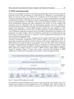
Our experimental conditions are listed in Fig. 12. As introduced before, Sensing Room, shown

at the left part of Fig. 12, was our test environment. Throughout the experiments, four objects,
shown at the top left part of Fig. 12, were selected as typical daily objects, which were a
nail clipper, a mug, a coffee mill, and a stuffed animal. On each object, an active RFID tag
including a vibration sensor was attached. Also we assumed 13 locations where objects would
be placed and five readers installed at different places. For pattern recognition, we constructed
a learning database with about 18,000 data sets stored in it. In more detail, the same amount
of RSSI datasets of each location of the labeled 13 locations were stored as training datasets.
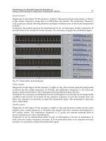
In the experiment, a participant leaded a typical daily life using four objects with active
RFID tags attached shown in Fig. 13. The system was supposed to estimate the location
of each object every sampling frame. The total number of targeted frames was 2520. To
provide the localization performance through a sequence of daily activity, we defined the
ratio of the number of correctly estimated frames to the total number of targeted frames
as the performance metric (Eq.2). In this case, "correct frame" means the frame that both
identification and localization succeeded. Furthermore, throughout the experiment, we only
adopted first location candidate and ignored the second and third location candidates in order
to provide a more reliable indicator of object localization.
Accuracy
[%]=
Correct N umbero f Fr ames
To talN umbero f Fr ames
(2)
232
Deploying RFID – Challenges, Solutions, and Open Issues
Use of Active RFID and Environment-Embedded Sensors for Indoor Object Location Estimation 15
Test Environment (Sensing Room)
•Objects
•Locations
13 labeled items in diagram
•RF Readers
5 readers marked

with arrows in diagram
•Training Data in Learning Database
13 (locations) × 1420 (datapoints)
=18460(datapoints)
Sink
Fridge
Cabinet
Shoes
Cupboard
Kitchen
Cabinet
Bed
Table
Sofa
Shelf
StereoShelf
Desk Cabinet
Desk
TV Shelf
RF Reader
active RFID tags
500 cm
450 cm
Fig. 12. Experiment Conditions
Vibration Sensor: OFF→ON
Target Object: Coffee Mill
Correct Label:
Move from Cabinet
Vibration Sensor: ON→OFF
Table Sensor: OFF→ON

Target Object: Coffee Mill
Correct Label:
Place on Table
Vibration Sensor: OFF→ON
Switch Sensor OFF→ON
Target Object: Mug
Correct Label:
Draw from Cabinet
Vibration Sensor: ON→OFF
Target Object: Mug
Correct Label:
Place on Kitchen Cabinet
Vibration Sensor: OFF→ON
Table Sensor: ON→OFF
Target Object: Coffee Mill
Correct Label:
Move from Table
Vibration Sensor: ON→OFF
Target Object: Coffee Mill
Correct Label:

Place on Kitchen Cabinet
Vibration Sensor: ON→OFF
Target Object: Mug
Correct Label:
Place in Sink
Vibration Sensor: OFF→ON
Switch Sensor OFF→ON
Target Object: Nail Clipper
Correct Label:

Draw from Cabinet
Vibration Sensor: ON→OFF
Sofa Sensor: OFF→ON
Target Object: Nail Clipper
Correct Label:
Place on Sofa
Vibration Sensor: ON→OFF
Switch Sensor OFF→ON
Target Object: Nail Clipper
Correct Label:
Put into Cabinet
Vibration Sensor: OFF→ON
Switch Sensor OFF→ON
Target Object: Stuffed Animal
Correct Label:
Draw from Cabinet
Vibration Sensor: ON→OFF
Target Object: Stuffed Animal
Correct Label:
Place on Desk
Start
End
Fig. 13. Experiment Scenes
4.3 Results and discussion
We classified the estimation results by the pattern recognition method used for the localization
and by the types of information used for the estimation, as shown in Table 3. There was
233
Use of Active RFID and Environment-Embedded Sensors for Indoor Object Location Estimation
16 Will-be-set-by-IN-TECH
(Data from floor, table, sofa, switch, and vibration sensors)

RSSI Data Only RSSI and Sensor Data RSSI and Sensor Data (w/o Floor Sensor)
KNN 50.2% 97.0% 95.3%
DKNN 49.6% 97.0% 95.3%
3-layered NN 22.0% 98.6% 90.6%
Table 3. Location Estimation Results (Only first location candidate is allowed)
(Data from floor, table, sofa, switch, and vibration sensors)
RSSI Data Only RSSI and Sensor Data RSSI and Sensor Data (w/o Floor Sensor)
KNN 60.3% 100.0% 95.3%
DKNN 61.2% 100.0% 95.3%
3-layered NN 36.5% 100.0% 92.6%
Table 4. Location Estimation Results (Up to third location candidate is allowed)
little difference in the results among the pattern recognition method used: KNN, DKNN,
and three-layered NN algorithm. There was a substantial difference in the results among
the pattern recognition methods used for the estimation. Localization accuracy with only
RSSI of the active RFID was 50% at best, whereas when we combined these two approaches
followed our proposed estimation algorithm, the accuracy reached 97.0% regardless of the
pattern recognition method. With the three-layered NN algorithm, it reached 98.6% at best.
Although we used floor sensors for the estimation in the best case, the system still recorded
95.3% even without floor sensors as shown in the table.
The results shown in Table.3 suggest two things in particular. One is that the pattern
recognition method used has little effect on the location estimation accuracy. Although we
used three kinds of methods such as k-nearest neighbor (KNN), distance-weighted k-nearest
neighbor (DKNN), and three-layered neural network (NN), none of them achieved sufficient
accuracy in object localization. The main cause of estimation mistakes we suppose is that the
object location is far from all the RF readers. As the radio wave is sensitive to environmental
noises, the further the distance between tag and reader is, the more unreliable RSSI becomes.
The other thing which we noticed from the results is that the lack of estimation accuracy
caused by not using floor sensor data can be approximately compensated for by using the
proposed algorithms and other simple sensors instead of floor sensors. Although floor sensors
can detect human position accurately, they are costly and require complicated maintenance.

To reduce the cost and maintenance burden, we estimated object location by using only the
RSSI data and data from other simple sensors (table, sofa, and switch sensors). The results
indicate that data from a combination of these sensors can achieve accuracy almost equal to
that of using floor sensors.
To make a comparison, we conducted another experiment using exactly the same data as the
previous experiment. In this case, not only the first location candidate but also the second and
the third location candidates were counted. The result is shown in Table 4.
The result shown in Table 4 indicates that the estimation performance does not make a big
difference between single location candidate and plural location candidates. Of course, when
we allow the second and the third location candidates, the estimation performance improves
to some extent. However the improvement is too slight to make a significant impact on the
estimation performance of our system.
Although we conducted all the experiments in Sensing Room, our object location estimation
method does not rely on either the experimental environment or the kinds of sensors. That is
234
Deploying RFID – Challenges, Solutions, and Open Issues
Use of Active RFID and Environment-Embedded Sensors for Indoor Object Location Estimation 17
to say, our method can work well in any houses as long as the sensors embedded in the house
can detect the same kinds of human behavior.
5. Conclusion
In conclusion, we have developed an indoor object localizing method by using active RFID
tags and simple switch sensors embedded in the environment. Our system uses 1) a pattern
recognition approach to classify the RSSIs collected from several RF readers into a particular
location, and 2) the information detected by vibration sensors and environment-embedded
sensors to improve the robustness of the method. Although position sensors used in our
previous work can detect accurate human position in the environment, we attempted to
eliminate them because of their disadvantages by combining simple switch sensors. The
results show that our method can be used to estimate the location of daily objects with
sufficient accuracy without the use of the position sensors.
One of future work is to reduce the number of RF readers. In our work, we use five active RFID

readers placed at different locations so as to cover the whole environment. However, because
the unit cost of RF readers is quite expensive, we have to reduce the number of RF readers to
ease the economical burden on introducing our system without lowering the performance of
object location estimation.
6. References
Cover, T. & Hart, P. (1967). Nearest neighbor pattern classification, Information Theory, IEEE
Transactions on 13(1): 21 – 27.
Hightower, J., Borriello, G. & Want, R. (2000). SpotON: An indoor 3d location sensing
technology based on rf signal strength, Technical Report UW CSE 2000-02-02,
University of Washington.
Mori, T., Noguchi, H., Takada, A. & Sato, T. (2006). Sensing room environment: Distributed
sensor space for measurement of human dialy behavior, Transaction of the Society of
Instrument and Control Engineers E-S-1(1): 97–103.
Mori, T., Siridanupath, C., Noguchi, H. & Sato, T. (2007). Active rfid-based
object management system in sensor-embedded environment, FGCN2007Workshop:
International Symposium on Smart Home (SH’07), Jeju Island, Korea, pp. 25–30.
Mori, T., Takada, A., Noguchi, H., Harada, T. & Sato, T. (2005). Behavior prediction based
on daily-life record database in distributed sensing space, International Conference on
Intelligent Robots and Systems, pp. 1833–1839.
Ni, L. M., Liu, Y., Lau, Y. C. & Patil, A. P. (2004). Landmarc: Indoor location sensing using
active rfid, Wireless Networks 10(6): 701–710.
Pao, T L., Cheng, Y M., Yeh, J H., Chen, Y T., Pai, C Y. & Tsai, Y W. (2008). Comparison
between weighted d-knn and other classifiers for music emotion recognition,
International Conference on Innovative Computing Information and Control(ICICIC’08),
pp. 530–530.
Shih, S T., Hsieh, K. & Chen, P Y. (2006). An improvement approach of indoor location
sensing using active rfid, the First International Conference on Innovative Computing,
Information and Control(ICICIC’06), pp. 453–456.
235
Use of Active RFID and Environment-Embedded Sensors for Indoor Object Location Estimation

18 Will-be-set-by-IN-TECH
Shimodaira, H. (1994). A weight value initialization method for improving learning
performance of the backpropagation algorithm in neural networks, International
Conference on Tools for Artificial Intelligence (ICTAI), pp. 672–675.
yao Jin, G., yi Lu, X. & Park, M S. (2006). An indoor localization mechanism using active
rfid tag, IEEE International Conference on Sensor Networks, Ubiquitous, and Trustworthy
Computing(SUTC’06), pp. 40–43.
Zhao, Y., Liu, Y. & Ni, L. M. (2007). Vire: Active rfid-based localization using virtual reference
elimination, International Conference on Parallel Processing (ICPP’07), pp. 56–63.
236
Deploying RFID – Challenges, Solutions, and Open Issues
0
RFID Sensor Modeling by Using
an Autonomous Mobile Robot
Grazia Cicirelli, Annalisa Milella and Donato Di Paola
Institute of Autonomous Systems for Automation (National Research Council)
Italy
1. Introduction
Radio Frequency Identification (RFID) technology has been available for more than fifty years.
Nevertheless, only in the last decade, the ability of manufacturing the RFID devices and
standardization in industries have given rise to a wide application of RFID technology in
many areas, such as inventory management, security and access control, product labelling
and tracking, supply chain management, ski lift access, and so on.
An RFID device consists of a number of RFID tags or transponders deployed in the
environment, one or more antennas, a receiver or reader unit, and suitable software for
data processing. The reader communicates with the tags through the scanning antenna that
sends out radio-frequency waves. Tags contain a microchip and a small antenna. The reader
decodes the signal provided by the tag, whereas the software interprets the information
stored in the tagŠs memory, usually related to its unique ID, along with some additional
information. Compared to conventional identification systems, such as barcodes, RFID tags

offer several advantages, since they allow for contactless identification, cheapness, reading
effectiveness (no need of line of sight between tags and reader). Furthermore, passive
tags work without internal power supply and have, potentially, a long life run. Owing to
these advantageous properties, RFID technology has recently attracted the interest of the
mobile robotics community that has started to investigate its potential application in critical
navigation tasks, such as localization and mapping. For instance, in (Kubitz et al., 1997) RFID
tags are employed as artificial landmarks for mobile robot navigation, based on topological
maps. In (Tsukiyama, 2005), the robot follows paths using ultrasonic rangefinders until an
RFID tag is found and then executes the next movement according to a topological map. In
(Gueaieb & Miah, 2008), a novel navigation technique is described, but it is experimentally
illustrated only through computer simulations. Tags are placed on the ceiling in unknown
positions and are used to define the trajectory of the robot that navigates along the virtual line
on the ground, linking the orthogonal projection points of the tags on the ground. In (Choi
et al., 2011) a mobile robot localization technique is described, which bases on a sensor fusion
that uses an RFID system and ultrasonic sensors. Passive RFID tags are arranged in a fixed
pattern on the floor and absolute coordinate values are stored in each tag. The global position
of the mobile robot is obtained by considering the tags located within the reader recognition
area. Ultrasonic sensors are used to compensate for limitations and uncertainties in RFID
system.
13
2 RFID
Although effective in supporting mobile robot navigation, most of the above approaches
either assume the location of tags to be known a priori or require tags to be installed in order
to form specific patterns in well-structured environments. Nevertheless, in real environments
this is not always possible. In addition, due to the peculiarities of these approaches, no sensor
model is presented, because they use only the identification event of RFID tags, without
considering at what extent. On the other hand, modelling RFID sensors and localizing passive
tags is not straightforward. RFID systems are usually sensitive to interference and reflections
from other objects. The position of the tag relative to the receivers also influences the result of
the detection process, since the absorbed energy varies accordingly. These undesirable effects

produce a number of false negative and false positive readings that may lead to an incorrect
belief about the tag location and, eventually, could compromise the performance of the overall
system (Brusey et al., 2003; Hähnel et al., 2004).
Algorithms to model RFID system have been developed by a few authors. They use different
approaches that varies depending on the type of sensor information used and the method
applied to model this information. Earlier works model the sensor information considering
only tag detection event. More recent ones, instead, consider also the received signal strength
(RSSI) value. This difference is principally due to the evolution of new RFID devices.
Nevertheless, in some cases the RSSI is simulated by means of the different power levels of
the antenna (Alippi et al., 2006; Ni et al., 2003). (Alippi et al., 2006), for example, suggest a
polar localization algorithm based on the scanning of the space with rotating antennas and
several readers. At each angular value the antenna is provided with an increasing power by
the reader. At the end of each interrogation campaign from each reader, the processing server
obtains, for each tag, a packet containing the reader ID, the angular position, the tag ID and
the minimum detection power.
One of the first works dealing with RFID sensor modeling is the one proposed in (Hähnel
et al., 2004). The sensor model is based on a probabilistic approach and is learnt by generating
a statistics by counting the frequency of detection given different relative position between
antenna and tag. In (Liu et al., 2006) the authors present a simplified antenna model that
defines a high probability region, instead of describing the probability at each location, in
order to achieve computational efficiency. In (Vorst & Zell, 2008) the authors present a novel
method of learning a probabilistic RFID sensor model in a semi-autonomous fashion.
A novel probabilistic sensor model is also proposed in (Joho et al., 2009). RSSI information and
tag detection event are both considered to achieve a higher modelling accuracy. A method for
bootstrapping the sensor model in a fully unsupervised manner is presented. Also, in (Milella
et al., 2008) a sensor model is illustrated. The presented approach differs from the above in
that they use fuzzy set theory instead of probabilistic approach.
In this chapter we present our recent advances in fuzzy logic-based RFID modelling using an
autonomous robot. Our work follows in principle the work by (Joho et al., 2009), since we
use both signal strength information and tag detection event for sensor modelling. However,

our approach is different in that is based on a fuzzy reasoning framework to automatically
learn the model of the RFID device. Furthermore, we consider not only the relative distance
between tag and antenna, but also their relative orientation.
The main contribution of our work concerns supervised learning of the model of the RFID
reader to characterize the relationship between tags and antenna. Specifically, we introduce
the learning of the membership function parameters that are usually empirically established
by an expert. This process can be inaccurate or subject to the expert’s interpretation. To
overcome this limitation, we propose to extract automatically the parameters from a set of
238
Deploying RFID – Challenges, Solutions, and Open Issues
RFID Sensor Modeling by Using
an Autonomous Mobile Robot 3
Fig. 1. The mobile robot Pioneer P3AT equipped with two RFID antennas and a laser range
scanner.
training data. In particular, Fuzzy C-Means (FCM) algorithm is applied to automatically
cluster sample data into classes and also to obtain initial data memberships. Next, this
information is used to initialize an ANFIS neural network, which is trained to learn the RFID
sensor model. The RFID sensor model is defined as combination of an RSSI model and a Tag
Detection Model. Experimental results from tests performed in our Mobile Robotics Lab are
presented. The robot used in the experimental session is a Pioneer P3AT equipped with two
RFID antennas and a laser range scanner (see Fig. 1). The RFID system is composed by a SICK
RFI 641 UHF reader and two antennas, whereas tags are passive UHF tag ¸SDogBone" by UPM
Raflatac.
The rest of this chapter is organized as follows. Section 2 describes the sensor modelling
approach. Experimental results are shown in Section 3. Finally, conclusions are drawn in
Section 4.
2. Learning the Sensor Model
In our work, modeling an RFID device means to model the possibility of detecting a tag given
its relative position and angle with respect to the antenna. Building this sensor model involves
two phases: data acquisition and model learning. The former refers to the strategy we apply in

239
RFID Sensor Modeling by Using an Autonomous Mobile Robot
4 RFID
order to collect data. The latter, instead, refers to the construction of the model actually learnt
by using recorded data. To model the RFID device we use a Fuzzy Inference System and then
to learn it the Adaptive Neuro-Fuzzy Inference System (ANFIS) is applied: the membership
function parameters and the rule base are automatically learnt by training an ANFIS neural
network on sample instances removing, in this way, the subjectivity of an observer. First
sample data are automatically clustered into classes by using the Fuzzy C-Means (FCM)
algorithm that at the same time gives an initial fuzzy inference system. Next this information
is used to initialize the ANFIS neural network. In the subsequent, both algorithms FCM and
ANFIS will be briefly reviewed before the sensor model description.
2.1 Data recording
Past approaches to data recording, presented in related works (Hähnel et al., 2004; Milella
et al., 2008), fix a discrete grid of different positions and count frequencies of tag detections for
each grid cell. These detections are collected by moving a robot, equipped with one or more
antennas, on this grid in front of a tag attached to a box or a wall. This way of proceeding
is advantageous in that measurements are taken at known positions and detection rates are
computed as tag detection frequencies on a grid. However, this procedure could be tedious
and slow if a huge quantity of measurements has to be taken. We follow a slightly different
approach to collect the data useful for the sensor model construction. After having deployed
a number of tags at different positions in our corridor-like environment, the robot, equipped
with the antennas, is manually moved up and down the corridor, continuously recording
tag measurements. With tag measurements we refer to the relative distance and relative
orientation of the antenna with respect to the tag and RSSI value for each tag detection.
Notice that, for each detected tag, the reader reports the tag ID, the RSSI value and which
antenna detected the tag. True tag locations are computed by using a theodolite station,
whereas the robot positions, in a map of the environment, are estimated applying an accurate
self-localization algorithm called Mixture-Monte Carlo Localization (Thrun et al., 2000) by
using laser data. Then the relative position between tags and robot are known. Notice that

more tags can be simultaneously read by the antenna, therefore the recording phase is, at the
same time, rich in data and faster with respect to the above reported ones. In addition, the
proposed approach skips the tedious effort of choosing grid points, since a variety of positions
for the robot (or antennas) is guaranteed during the guided tour of the environment.
2.2 Fuzzy C-Means (FCM)
FCM is one of the most popular family of clustering algorithms that is C-Means (or K-Means),
where C refers to the number of clusters. These algorithms base on the minimum assignment
principle, which assigns data points to the clusters by minimizing an objective function
that measures the distance between points and the cluster centers. The advantages of
these algorithms are their simplicity, efficiency and self-organization. FCM is a variation of
C-Means. It was introduced in (Bezdek, 1981). The peculiarity of fuzzy clustering is that data
points do not belong to exactly one cluster, but to more than one cluster since each point has
associated a membership grade which indicates the degree to which it belongs to the different
clusters.
Given a finite set of data point vectors Z
= {Z
1
, Z
2
, , Z
N
}, FCM algorithm partitions it into
a collection of C
≤ N clusters such that the following objective function is minimized:
J
q
=
C
∑
i=1

N
∑
k=1
w
q
ik
Z
k
− V
i

2
240
Deploying RFID – Challenges, Solutions, and Open Issues
RFID Sensor Modeling by Using
an Autonomous Mobile Robot 5
where V
i
are the cluster centers for i = 1, C; w
ik
is the membership value whit which point
Z
k
belongs to the cluster defined by V
i
center and q > 1 is the fuzzification parameter. This
parameter in general specifies the fuzziness of the partition, i.e. larger the value of q greater is
the overlap among the clusters.
Starting by an initial guess for the cluster centers, FCM algorithm alternates between
optimization of J

q
over the membership values w
ik
fixed the cluster centers V
i
and viceversa.
Iteratively updating w
ik
and V
i
, FCM moves the cluster centers to the optimal solution within
the data set. Membership values and cluster centers are computed as follows:
w
ik
=

D
2
ik
∑
C
j
=1
D
2
jk

−1
q−1
under the constraint

∑
C
i
=1
w
ik
= 1 ∀k
V
i
=
∑
N
k
=1
w
q
ik
Z
k
∑
N
k
=1
w
ik
for i = 1, , C
where D
ik
is the distance between i-th cluster center and k-th sample point. The iterative
process ends when the membership values and the cluster centers for successive iterations

differ only by a predefined tolerance .
2.3 Adaptive Neuro Fuzzy Inference System (ANFIS)
ANFIS (Jang, 1993) implements a Sugeno neuro-fuzzy system making use of a hybrid
supervised learning algorithm consisting of backpropagation and least mean square
estimation for learning the parameters associated with the input membership functions.
A typical i
− th if-then rule in a Takagi and Sugeno fuzzy model is of the type:
if x
1
is A
i
and x
2
is B
i
then f
i
= p
i
x
1
+ q
i
x
2
+ r
i
where A
i
and B

i
are the linguistic terms associated with the input variables x
1
and x
2
. The
parameters before the word ¸Sthen" are the premise parameters, those after ¸Sthen" are the
consequent parameters. Thereafter the case of two input variables x
1
and x
2
and two if-then
rules is considered for simplicity. The main peculiarity of a Sugeno fuzzy model is that the
output membership functions are either linear or constant.
The architecture of the ANFIS network is composed by five layers as shown in figure 2.
Layer 1 The first layer is the input layer and every node has a node function defined by
the membership functions of the linguistic labels A
i
and B
i
. Usually the generalized bell
membership function:
μ
A
i
(x)=
1
1 +(
x−c
i

a
i
)
2b
i
or the Gaussian function is chosen as node function:
μ
A
i
(x)=e
−(
x−c
i
a
i
)
2
where a
i
, b
i
and c
i
are the premise parameters. The same holds for μ
B
i
(x).
Layer 2 In the second layer each node computes the firing strength or weight of the
corresponding fuzzy rule as product of the incoming signals.
w

i
= μ
A
i
(x
1
)μ
B
i
(x
2
) i = 1,2
Each node of this layer represents the rule antecedent part.
241
RFID Sensor Modeling by Using an Autonomous Mobile Robot
6 RFID
Fig. 2. The ANFIS architecture.
Layer 3 The third layer normalizes the rule weights considering the ratio between the i-th
weight and the sum of all rule weights:
w
i
=
w
i
∑
i
w
i
i = 1,2
Layer 4 In the fourth layer the parameters of the rule consequent parts are determined. Each

node produces the following output:
w
i
f
i
= w
i
(p
i
x
1
+ q
i
x
2
+ r
i
)
where {p
i
, q
i
, r
i
} are the consequent parameters.
Layer 5 Finally the fifth layer computes the overall output as following:
f
=
∑
i

w
i
f
i
=
∑
i
w
i
f
i
∑
i
w
i
In this work we use Gaussian membership functions and their parameters, the premise
parameters, are initialized by using the FCM algorithm described in the previous section.
Training the network consists of determining the optimal premise and consequent parameters.
During the forward pass the consequent parameters of layer 4 are identified by least square
estimate. In the backward pass, instead, the premise parameters are updated applying
gradient descent. For more details see (Jang, 1993).
2.4 Sensor Model
Our RFID system, at each tag detection event returns two pieces of information: the tag unique
ID and its signal strength. Note that receiving a signal strength measurement implicitly
involves that a tag has been detected, but we consider both information in order to make
a distinction among the different tags deployed in the environment. However in the rest of
the paper, for simplicity, all the variables that will be defined will refer to a generic unique tag,
assuming that only relative pose between tag and antenna is relevant. This last assumption is
242
Deploying RFID – Challenges, Solutions, and Open Issues

RFID Sensor Modeling by Using
an Autonomous Mobile Robot 7
Fig. 3. Relative pose between tag and antenna.
a strong one since, as discussed in the introduction section, the propagation of an RFID signal
is influenced by a set of factors dependent on the particular location of each tag: for example
the materials the tag is attached on or the surface materials around the tag that can reflect
or absorb the electromagnetic waves or the orientation of the tag. While location-dependent
models certainly provide more precision they involve a high computational cost. In this work
we tried to find a good trade-off between computational overhead and precision, developing
a model that bases on both the relative location and the relative orientation of the antenna
with respect to the tag.
First of all some variable definitions are needed: we define α the relative orientation between
antenna and tag (see Figure 3). As shown in figure 3 points A and T are antenna and tag
position in the world reference system X
w
OY
w
, whereas d is the distance between T and
A. Angle θ
A
is the absolute orientation of the antenna in the world reference system. Each
antenna is mounted on the robot and its pose with respect to the robot is known, therefore θ
A
as well as each antenna position is simply obtained by using the absolute pose of the robot in
the X
w
OY
w
system.
As introduced before the sensor model specifies the possibility of detecting a tag given the

relative position between antenna and tag. This is modelled by multiplying the expected
signal strength f
s
(d, α) and the frequency f
T
(d, α) of detecting a tag T given a certain distance
d and a certain relative orientation α between tag and antenna. In formula:
ρ
= f
s
(d, α)f
T
(d, α) (1)
In other words the sensor model is obtained combining an RSSI Model (SSM) and a Tag
Detection Model (TDM). These two models are learnt by using Fuzzy Inference System,
applying ANFIS networks. Both models are detailed in the next two subsections.
2.4.1 RSSI Model (SSM)
RSSI Model is learnt applying the ANFIS network with two inputs, d and α, and one output f
s
.
Data samples used as input to FCM and ANFIS are the ones stored during the data acquisition
243
RFID Sensor Modeling by Using an Autonomous Mobile Robot
8 RFID
Fig. 4. Input-Output surface for RSSI Model.
phase, as described in section 2.1. First FCM algorithm is applied to initialize the membership
function parameters of the input variables considering C
= 3 clusters (see section 2.2), then
ANFIS is trained by using an additional training data set with 12395 samples. Each training
data sample is composed by the couple of input variables

(d, α) and by the relative signal
strength s, stored during data acquisition, opportunely normalized in [0,1]. For simplicity
data with distance d
< 3meters has been considered. Figure 4 shows the surface that models
the if-then rules of the obtained fuzzy inference system. Lighter areas denote higher received
signal strength.
2.4.2 Tag Detection Model (TDM)
Tag Detection Model has been built similarly to RSSI model. The input variables are the same
(d, α), whereas the output variable is the frequency f
T
of detecting a tag given d and α.In
order to build the training set, the proper f
T
value must be associated to each couple (d, α).
This has been done by first discretizing the space into a grid of cells and then counting the
number of tag detection events ( n
+
T
) and the number of no-tag detection events (n
−
T
). For each
cell the frequency value f
T
is evaluated by using its definition formula:
f
T
=
n
+

T
n
+
T
+ n
−
T
FCM, with C = 3 (see section 2.2), is then applied on a first training set of data to obtain an
initial fuzzy inference system used as input for ANFIS network. A second training set with
12395 sample data is used to train the network. In this case each sample is composed by the
input couple
(d, α) and the output value f
T
. The obtained input-output surface is displayed
in figure 5.
3. Experiments
Some tests have been carried out in our laboratory by using the Pioneer P3AT robot shown in
figure 1. The robot has been moved randomly in front of a tag. During navigation a number
of points P
i
for i = 1, , M have been generated uniformly distributed within a circular area
around each robot pose. Knowing the absolute position and orientation of the robot and the
244
Deploying RFID – Challenges, Solutions, and Open Issues
RFID Sensor Modeling by Using
an Autonomous Mobile Robot 9
Fig. 5. Input-Output surface for Tag Detection Model.
absolute position of each generated point, the distance and relative orientation between each
point P
i

and each antenna can be estimated. These data are used as input to the RFID sensor
model and the output ρ
i
is obtained for each P
i
. Figure 6 shows some plots of the described
procedure in different poses of the robot. For clarity of display, data relative to only one
antenna are plotted. In particular in each plot the green points refer to the set of randomly
generated points, the red oriented triangle is the antenna, the blue star point denotes the
position of one tag. The green area of each point changes depending on the confidence value
ρ
i
defined by the sensor model. Higher ρ
i
larger the green area around point P
i
. As can be
seen in figure 6 larger areas are for those points close to the antenna current position and in
front of it. Points located behind the antenna have very low ρ
i
values and then are represented
by smaller green areas.
At the same time, during navigation, the signal strengths s
j
received by the RFID reader have
been stored and compared with the f
s
values returned by the RSSI model. More specifically a
path of 200 robot poses Q
j

, for j = 1, , 200, has been considered and for each pose the average
¯
f
j
s
has been estimated considering only those points localized close to the tag:
¯
f
j
s
=
∑
k∈P
f
k
s
|P|
where P = {P
i
: P
i
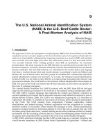
− T < 10cm}. Figure 7 shows the error Error = |
¯
f
j
s
− s
j
| estimated in
each robot pose. As can be noticed the error is below 20% which is a good result considering

the high fluctuations of RSSI signals. Furthermore this proves the high reliability of RSSI
model and then of RFID sensor model which combines both SSM and TDM.
4. Conclusion
In this chapter an approach for developing an RFID sensor model has been presented. The
model is a combination of an RSSI model and a tag Detection model. The main contribution
of our work concerns the supervised learning of the model to characterize the relationship
between tags and antenna. FCM and ANFIS networks have been used to learn the Fuzzy
Inference Systems describing both SSM and TDM. Experimental tests prove the reliability of
245
RFID Sensor Modeling by Using an Autonomous Mobile Robot
10 RFID
Fig. 6. Sample pictures of points randomly deployed around different robot poses with
plotted importance weights (green blobs). The red oriented triangle is one antenna placed on
the robot, the blue star point is the tag.
246
Deploying RFID – Challenges, Solutions, and Open Issues
RFID Sensor Modeling by Using
an Autonomous Mobile Robot 11
Fig. 7. Percentage average error on f
s
values vs. robot poses.
the obtained model. Constructing a reliable sensor model is very important for successive
applications such as tag localization, robot localization, just to mention a few. Our future
work, in fact, will address these two problems: automatic localization of tags displaced in
unknown positions of the environment and, successively, absolute robot localization.
5. References
Alippi, C., Cogliati, D. & Vanini, G. (2006). A statistical approach to localize passive rfids,
IEEE International Symposium on Circuits and Systems, Island of Kos, Greece.
Bezdek, J. C. (1981). Pattern Recognition with Fuzzy Objective Function Algorithms, Plenum, New
York.

Brusey, J., Floerkemeier, C., Harrison, M. & Fletsher, M. (2003). Reasoning about uncertainty
in location identification with rfid, IJCAI-03 Workshop on Reasoning with Uncertainty
in Robotics.
Choi, B. S., Lee, J. W., Lee, J. J. & Park, K. T. (2011). A hierarchical algorithm for indoor mobile
robots localization using rfid sensor fusion, IEEE Transactions on Industrial Electronics
to appear.
Gueaieb, W. & Miah, M. S. (2008). An intelligent mobile robot navigation technique using rfid
technology, IEEE Transactions on Instrumentation and Measurement Vol. 57(No. 9).
Hähnel, D., Burgard, W., Fox, D., Fishkin, K. & Philipose, M. (2004). Mapping and
localization with rfid technology, IEEE International Conference on Robotics and
Automation (ICRA2004), New Orleans, LA, USA.
Jang, S. R. (1993). Anfis: adaptive-network-based fuzzy inference system, IEEE Trnas. on
Systems, Man and Cybernetics Vol. 23(No. 3): 665–685.
Joho, D., Plagemann, C. & Burgard, W. (2009). Modeling rfid signal strength and tag detection
for localization and mapping, IEEE International Conference on Robotics and Automation
(ICRA2009), Kobe, Japan.
247
RFID Sensor Modeling by Using an Autonomous Mobile Robot
12 RFID
Kubitz, O., Berger, M., Perlick, M. & Dumoulin, R. (1997). Application of radio frequency
identification devices to support navigation of autonomous mobile robots, IEEE 47th
Vehicular Technology Conference, Phoenix, Arizona, USA, pp. 126–130.
Liu, X., Corner, M. & Shenoy, P. (2006). Ferret: Rfid localization for pervasive multimedia, 8th
UbiComp Conference, Orange County, California, USA.
Milella, A., Cicirelli, G. & Distante, A. (2008). Rfid-assisted mobile robot system for mapping
and surveillance of indoor environments, Industrial Robot: An International Journal
Vol. 35(No. 2): 143–152.
Ni, M. L., Liu, Y., Lau, Y. C. & Patil, A. P. (2003). Landmarc: Indoor location sensing using
active rfid, IEEE International Conference on Pervasive Computing and Communications,
Fort Worth, Texas, USA.

Thrun, S., Fox, D., Burgard, W. & Dellaert, F. (2000). Robust monte carlo localization for mobile
robots, Artificial Intelligence Vol. 128(No. 1-2): 99–141.
Tsukiyama, T. (2005). World map based on rfid tags for indoor mobile robots, Proceedings of
the SPIE, Vol. Vol. 6006, pp. 412–419.
Vorst, P. & Zell, A. (2008). Semi-autonomous learning of an rfid sensor model for mobile robot
self-localization, European Robotics Symposium, Vol. Vol. 44/2008 of Springer Tracts in
Advanced Robotics, Springer, Berlin/Heidelberg, pp. 273–282.
248
Deploying RFID – Challenges, Solutions, and Open Issues
14
Location of Intelligent Carts Using RFID
Yasushi Kambayashi and Munehiro Takimoto
Nippon
Institute of Technology & Tokyo University of Science
Japan
1. Introduction
This chapter addresses optimizing distributed robotic control of systems using an example
of an intelligent cart system designed to be used in common airports. This framework
provides novel control methods using mobile software agents. In airport terminals, luggage
carts used by traveler are taken from a depot but are left after use at arbitrary points. It
would be desirable that carts be able to draw themselves together automatically after being
used so that manual collection becomes less laborious. In order to avoid excessive energy
consumption by the carts, we employ mobile software agents and RFID (Radio Frequency
Identification) tags to identify the location of carts scattered in a field and then cause them to
autonomously determine their moving behavior using a clustering method based on the ant
colony optimization (ACO) algorithm.
When we pass through terminals of an airport, we often see carts scattered in the walkway
and employees manually collecting them one by one. It is a laborious task and not a
fascinating job. It would be much easier if carts were roughly gathered in any way before
the laborers begin to collect them. Multiple robot systems have made rapid progress in

various fields, and the core technologies of multiple robot systems are now easily available
(Kambayashi & Takimoto, 2005). Employing such technologies, it is possible to give each
cart minimum intelligence, making each cart an autonomous robot. We realize that for such
a system cost is a significant issue and we address one of those costs, the power source. A
big, powerful battery is heavy and expensive; therefore such intelligent cart systems with
small batteries are desirable to save energy (Takimoto, Mizuno, Kurio & Kambayashi, 2007;
Nagata, Takimoto & Kambayashi, 2009; Oikawa, Mizutani, Takimoto & Kambayashi, 2010;
Abe, Takimoto & Kambayashi, 2011).
Travelers pick up carts at designated points and leave them in arbitrary places. It is
desirable that intelligent carts (intelligent robots) draw themselves together automatically. A
simple implementation would be to give each cart a designated assembly point to which it
automatically returns when free. That solution is easy to implement, but some carts would
have to travel a long way back to their own assembly point, even though they are located
close to other assembly points. That strategy consumes unnecessary energy.
To improve efficiency, we employ mobile software agents to locate carts scattered in a field,
e.g. an airport, and enable them to determine their moving behavior autonomously using a
clustering algorithm based on ant colony optimization (ACO). ACO is a swarm intelligence-
based method and a multi-agent system that exploits artificial stigmergy for the solution of
combinatorial optimization problems. Preliminary experiments yield a favorable result. Ant

Deploying RFID – Challenges, Solutions, and Open Issues

250
colony clustering (ACC) is an ACO specialized for clustering objects. The idea is inspired by
the collective behaviors of ants, used by Deneubourg to formulate an algorithm that
simulates the ant corps gathering and brood sorting behaviors (Deneuburg, Goss, Franks,
Sendova-Franks, Detrain & Chretien, 1991).
We have studied the base idea for controlling mobile multiple robots connected by
communication networks (Kambayashi, Tsujimura, Yamachi, Takimoto, & Yamamoto, 2010;
Kambayashi & Takimoto, 2005). Our framework provides novel methods to control

coordinated systems using mobile agents. Instead of physical movement of multiple robots,
mobile software agents can migrate from one robot to another so that they can minimize
energy consumption for aggregation. In this chapter, we describe the details of
implementation of the multi-robot system using multiple mobile agents and static agents
that implement ACO as well as the location system using RFID. The combination of the
mobile agents augmented by ACO and mobile multiple robots with RFID opens a new
horizon of efficient use of mobile robot resources. We report here our experimental
observations of our robot cart system.
Quasi-optimal cart collection is achieved in three phases. The first phase collects the
positions of the carts. One mobile agent issued from the host computer visits scattered carts
one by one and collects the positions of them. The precise coordinates and orientation of
each robot are determined by interrogating RFID tags under the floor carpet. Upon the
return of the position collecting agent, the second phase begins wherein another agent, the
simulation agent, performs the ACC algorithm and produces the quasi-optimal gathering
positions for the carts. The simulation agent produces not only the assembly positions of the
carts but also the moving routes and waiting timings for avoiding collisions; i.e. the entire
behaviors of all the intelligent carts. The simulation agent is a static agent that resides in the
host computer. In the third phase, a number of mobile agents, the driving agents are issued
from the host computer. Each driving agent migrates to a designated cart, and drives the
cart to the assigned quasi-optimal position that was calculated in the second phase.
The behaviors of each cart are determined by the simulation agent. It is influenced, but not
determined, by the initial positions and the orientations of scattered carts, and is
dynamically re-calculated as the configuration of the field (positions of the carts in the field)
changes. Instead of implementing ACC with actual carts, one static simulation agent
performs the ACC computation, and then mobile agents distribute the sets of produced
driving instructions. Therefore our method eliminates unnecessary physical movement and
provides energy savings.
The structure of the balance of this paper is as follows. In the second section, we review the
history of research in this area. In the third section, we describe the controlling agent system
that performs the arrangement of the intelligent carts. The agent system consists of several

static and mobile agents. The static agents interact with the users and compute the ACC
algorithm and the simulation of the intelligent carts‘ behaviors. The other mobile agents
gather the initial positions of the robots and drive the carts to the assembly positions. The
fourth section describes how each robot determines its coordinates and orientation by
sensing RFID tags under the floor carpet. The fifth section describes the ACC algorithm we
have employed to calculate the quasi-optimal assembly positions and moving instructions
for each cart. Finally, in the sixth section, we summarize the work and discuss future
research directions.

Location of Intelligent Carts Using RFID

251
2. Background
Kambayashi and Takimoto have proposed a framework for controlling intelligent multiple
robots using higher-order mobile agents (Kambayashi & Takimoto, 2005). The framework
helps users to construct intelligent robot control software using migration of mobile agents.
Since the migrating agents are of higher order, the control software can be hierarchically
assembled while they are running. Dynamic extension of control software by the migration
of mobile agents enables the controlling agent to begin with relatively simple base control
software, and to add functionalities one by one as it learns the working environment. Thus
we do not have to make the intelligent robot smart from the beginning or make the robot
learn by itself. The controlling agent can send intelligence later through new agents. Even
though the dynamic extension of the robot control software using the higher order mobile
agents is extremely useful, such a higher order property is not necessary in our setting. We
have employed a simple, non-higher-order mobile agent system for our intelligent cart
control system. We previously implemented a team of cooperative search robots to show the
effectiveness of such a framework, and demonstrated that that framework contributes to
energy savings for a task achieved by multiple robots (Takimoto, Mizuno, Kurio &
Kambayashi, 2007; Nagata, Takimoto & Kambayashi, 2009; Oikawa, Mizutani, Takimoto &
Kambayashi, 2010; Abe, Takimoto & Kambayashi, 2011). Our simple agent system should

achieve similar performance.
Deneuburg formulated the biologically inspired behavioral algorithm that simulates the ant
corps gathering and brood sorting behaviors (Deneuburg, Goss, Franks, Sendova-Franks,
Detrain, & Chretien, 1991). His algorithm captured many features of the ant sorting
behaviors. His design consists of ants picking up and putting down objects in a random
manner. He further conjectured that robot team design could be inspired from the ant corps
gathering and brood sorting behaviors (Deneuburg, Goss, Franks, Sendova-Franks, Detrain,
& Chretien, 1991). Wang and Zhang proposed an ant inspired approach along this line of
research that sorts objects with multiple robots (Wang & Zhang, 2004).
Lumer improved Deneuburg’s model and proposed a new simulation model that was called
Ant Colony Clustering (Lumer, & Faieta, 1994). His method could cluster similar object into
a few groups. He presented a formula that measures the similarity between two data objects
and designed an algorithm for data clustering. Chen et al have further improved Lumer’s
model and proposed Ants Sleeping Model (Chen, Xu & Chen, 2004). The artificial ants in
Deneuburg’s model and Lumer’s model have considerable amount of random idle moves
before they pick up or put down objects, and considerable amount of repetitions occur
during the random idle moves. In Chen’s ASM model, an ant has two states: active state and
sleeping state. When the artificial ant locates a comfortable and secure position, it has a
higher probability of being in the sleeping state. Based on ASM, Chen has proposed an
Adaptive Artificial Ants Clustering Algorithm that achieves better clustering quality with
less computational cost.
Algorithms inspired by behaviors of social insects such as ants that communicate with each
other by the stigmergy are becoming popular (Dorigo & Gambardella, 1996). Upon
observing real ants’ behaviors, Dorigo et al found that ants exchanged information by laying
down a trail of a chemical substance (pheromone) that is followed by other ants. They
adopted this ant strategy, known as ant colony optimization (ACO), to solve various
optimization problems such as the traveling salesman problem (TSP) (Dorigo &
Gambardella, 1996). Our ACC algorithm employs pheromone, instead of using Euclidian
distance to evaluate its performance.