Application of Artificial Neural Network (ANN)
to Predict Soil Organic Matter Using Remote Sensing Data in Two Ecosystems

191
model improved the MAE and RMSE, which were 0.09 and 0.12 for rangeland and 0.01 and
0.09 for forested land, respectively. Overall, the ANN models explained greater variability
and had higher capacity to predict SOM because these models use the non-linear
relationships among inputs and output variables.
The developed ANN model for predicting the soil organic matter in the present study
explained 84% and 91% of the total SOM variability in the rangeland and forest landscapes
receptively. Overall, the results implied that the ANN modeling was successful in
identifying most of the remote sensing data, which influence soil organic matter. However,
our results also suggest that this methodology used for analyzing the data has wider
applicability and can be applied to other sites.




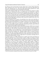
Fig. 4. Scatter plot displaying the relationships between measured and estimated value of the
SOM in MLR and ANN models at the two sites studied in west and central Iran. (a): MLR for
rangeland (b): MLR for forested land (c): ANN for rangeland, (d):ANN for forested land.
3.5 Determining the most important bands for explaining variability in SOM
The results on the relative importance of digital numbers and vegetation index using
sensitivity analysis based upon coefficients of sensitivity of the ANN model for soil organic
matter are shown in Fig. 5. The variables with high values made contributions to explain the
variability in SOM.
Band 1 of ETM was identified as the most important band for detecting SOM variability in
the study area of rangeland (Fig. 5a). Other important factors for predicting SOM, included

Biomass and Remote Sensing of Biomass

192
band 2 and 5 with relative coefficients of sensitivity ranking as 1.21 and 1.06, respectively.
Two other selected variables included band 7, and the NDVI showed sensitivity coefficient
of less than 1, implying that they make lower contribution in predicting SOM in the
rangeland site.
In the ANN analysis for SOM variability in forested land, the NDVI was identified as the
most important and other digital numbers were also identified. NDVI, a widely used
indicator in remote sensing showing abundance of vegetation cover. Spatial distribution of
the NDVI was strongly influenced by the relief, which controls the movement of water and
nutrients along the hillslopes. The distribution of vegetation could be controlled the
variability in SOM within the landscape, and the reflectance of soil surface in red and
infrared spectrums can determine the presence of different amounts of SOM. (Liu et al.,
2004). The NDVI indicates the greenness cover on the land surface and shows a well
documented relationship with crop and vegetation productivity (Pettorelli, 2005). Lozano-
Garcia et al. (1991) reported on the correlations between NDVI and soil properties. Li et al.
(2001) found that the NDVI between red and infrared wavelengths was cross-correlated
with soil water content, sand, clay and elevation. However, a composed and complex index
such as NDVI, which mostly reflects biomass status, indicates soil-dependent site quality
(Sommer, 2003).


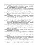
Fig. 5. Histogram displaying the results on sensitivity analysis, relative sensitivity
coefficients of remote sensing data for the SOM. NDVI: normalized difference vegetation
index.(a): Rangeland of Semiroum; (b): Forested land of Lordegan
Independent variable Landsat ETM digital numbers of bands 1, 2, 5 and 7, which may have
been influenced by the presence of vegetative cover, were identified as important factors for
the variability in SOM. Band 1 is useful for soil/vegetation differentiation and in
distinguishing the forest types. Band 2 detects green reflectance from healthy vegetation.
The two mid-IR red bands on TM ( bands 5 and 7) are useful for vegetation and soil
moisture studies (Lillesand &Kieffer, 1987).

Moreover, SOM has been related to reflectance in data collected over agricultural fields in
several studies (Coleman et al., 1991; Henderson, 1992; Chen, 2000) and it has been reported
that visible wave-lengths (0.425 to 0.695 mm) (Bands 1 to 3) had a strong correlation with
SOM for soils with the same parent material. The use of middle infrared bands (Band 5 of
ETM) improved the prediction of SOM content when the soils were from different parent
materials (Henderson, 1992). Chen et al. (2000) were able to accurately predict SOM using
true color imagery of a 115-ha field with the use of locally developed regression
relationships.
Application of Artificial Neural Network (ANN)
to Predict Soil Organic Matter Using Remote Sensing Data in Two Ecosystems

193
Organic matter influences soil optical properties. Organic matter may indirectly affect the
spectral influence, based on the soil structure and water retention capacity. High organic
matter in soil may produce spectral interferences for band characteristics of mineral like
manganese oxide and iron oxide (Coleman et al., 1991). The relationships of surface SOM
concentration with the pixel intensity values, with data ranging from 0 to 255 for each band,
were not linear (Chen, 2000). Therefore, non-linear regression analyses were developed.
Stamatiadis et al. (2005) observed that the red and NIR regions are more sensitive to
matterates in soils. The results of this study also showed that in samples that contain high
amounts of matterates, the visible bands showed higher correlation (Stamatiadis et al., 2005).
These results are similar to those reported by Fox and Sabbagh (2002) who found the
strongest correlation of SOM with reflectance in red band, but their results did not confirm
the result reported by Sullivan et al. (2005) and Agbu et al. (1990), who showed that
reflectance in green band was more strongly correlated with SOM than the reflectance in
red band. Krishnan et al. (1980), reported that no absorption climax was caused by organic
matter in the NIR region (800–2400 nm), and SOM content was better measured with visible
bands than NIR bands.
Overall, organic matter is the factor that influences soil optical properties. Organic matter
may indirectly affect the spectral influence, based on the soil structure and water retention

capacity. High organic matter in soil may produce spectral interferences for band
characteristics of minerals such as manganese and iron oxides.
The developed ANN models for predicting the SOM in the present study by ETM-Landsat
explained 84% and 91% of the total SOM variability within the two selected landscapes. A
part of the unexplained variability is probably due to the management practices such as
grazing and deforestation in some parts that influenced the plant density over the
landscape. Moreover, as reported by other researchers (Kaul et al., 2005), it is important to
compare the results of the ANN models with those obtained by other statistical approaches
for determining the precision of the model under development. Hence the learning rate,
number of hidden layer, number of hidden nodes and the training tolerance need to be
determined accurately for developing models for SOM prediction. However, the
performance of the ANN models as compared to other approaches suggest that ANN
models have better realistic chance to predict SOM, especially when complex non-linear
relationships exist among factors. In such cases, the correlation study may provide
inaccurate and even misleading results about the relationships (Liu et al., 2001).
4. Conclusions
In this study, the potential of remote sensing data for the estimation of within-field
variability of SOM was explored for hillslopes in the semiarid region under rangeland and
forested uses. Multivariate statistical techniques and ANNs were employed for model
development to explore the potential of remote sensing data. To achieve a nonlinear
function relating soil organic matter to remote sensing data in hilly region of the semiarid
region of central and western Iran, the results of this study indicated that the designed ANN
models was able to establish the relationship between the remote sensing data and SOM
content. Some of remote sensing data such as band 1, band 2 and NDVI were identified as
the important factors that explained the variability in SOM content at the sites studied both
in in rangeland and forested areas. The results showed that the MLR and ANN models
explained 54 and 84 % of the total variability in SOM, respectively, in the rangeland site.

Biomass and Remote Sensing of Biomass


194
On the other hand, the MLR and ANN models explained 77 and 91% of the total variability
of SOM in forested area using remotely sensed data.
The calculated MAE and RMSE values were 0.18 and 0.26 for the MLR model for SOM in
rangeland and 0.09 and 0.13 for the forested area using MLR. On the other hand, ANN
improved the MAE and RMSE to 0.09 and 0.12 for rangeland and 0.01 and 0.09 for forested
land, respectively. Therefore, the ANN model could provide superior predictive
performance when compared with the MLR model developed.
Our results also suggest that the future research should consider soil properties which are
used as factors in the equation, because soil reflectance properties depend on numerous soil
characteristics such as mineral composition, texture, structure and moisture content in the
use of remote sensing imagery to achieve a high accuracy in research.
5. References
Agbu, P. A.; Fehrenbacher, D. J. & Jansen, I. I. (1990). Soil property relationships with SPOT
satellite digital data in East Central Illinois. Soil Science Society of America Journal,
54, 807-812.
Blackmer, A. M. & White, S. E. (1998). Using precision farming technologies to improve
management of soil and fertilizer nitrogen. Australian Journal of Agricultural
Research, 49, 555–564.
Brown, D. J.; Shepherd, K. D.; Walsh, M. G.; Dewayne Mays, M. & Reinsch, T. G. (2006).
Global soil characterization with VNIR diffuse reflectance spectroscopy. Geoderma,
132, 273–290.
Caudill, H. J. (2006). Management and landscape influences on soil organic carbon in the
southern piedmont and coastal plain. the Graduate Faculty of Auburn University,
152.
Chang, C. W. & Laird, D. A. (2002). Near-infrared reflectance spectroscopic analysis of soil C
and N. Soil Science, 167, 110-116.
Chen, F.; Kissel, D. E.; West, L. T. & Adkins, W. (2000). Field-scale mapping of surface soil
organic carbon using remotely sensed imagery. Soil Science Society of America
Journal, 64, 746–753.

Chen, F.; Kissel, D. E.; West, L. T.; Rickman, D.; Luvall, J. C. & Adkins, W. (2005). Mapping
surface soil organic carbon for crop fields with remote sensing. Journal of soil and
water Conservation, 60, 51-57.
Christy, C. D.; Drummond, P. & Laird, D. A. (2003). An on-the-go spectral reflectance sensor
for soil. American Society of Agricultural Engineers Meeting, 3, 10-44.
Coleman, T. L.; Agbu, P. A.; Montgomery, O. L.; Gao, T. & Prasad, S. (1991). Spectral band
selection for quantifying selected proper-ties in highly weathered soils. Soil Science,
151 (5), 355-361.
Fox, G. A. & Sabbagh, G. J. (2002). Estimation of soil organic matter from red and near-
infrared remotely sensed data using a soil line Euclidean distance technique. Soil
Science Society of America Journal, 66, 1922-1929.
Galvao, L. S. & Vitorello, I. (1998). Role of organic matter in obliterating the effects of iron on
spectral reflectance and colour of Brazilian tropical soils. International Journal of
Remote Sensing, 19, 1969-1979.
Haykin, S. (1994). Neural Networks: A Comprehensive Foundation. Macmillan, New York,
NY.
Application of Artificial Neural Network (ANN)
to Predict Soil Organic Matter Using Remote Sensing Data in Two Ecosystems

195
Henderson, T. L.; Baumgardner, M. F.; Franzmeier, D. P.; Stott, D. E. & Coster, D. C. (1992).
High dimensional reflectance analysis of soil organic matter. Soil Science Society of
America Journal, 56, 865–872.
Huang, Y. (2009). Advances in Artificial Neural Networks – Methodological Development
and Application. Algorithms, 2, 973-1007.
Huete, A. R. & Escadafal, R. (1991). Assessment of biophysical soil properties through
spectral decomposition techniques. Remote Sensing of Environment, 35, 149-157.
Huete, A. R., Liu, H.Q. (1994). An error and sensitivity analysis of the atmospheric-
correcting and soil-correcting variants of the NDVI for the modis-eos. IEEE Trans.
Geosci. Remote Sensing, 32, 897-905.

Kaul, M.; Hill, R. & Walthall, C. (2005). Artificial neural networks for corn and soybean yield
prediction. Agricultural Systems, 85, 1-18.
Krishnan, P.; Alexander, J. D.; Butler, B. J. & Hummel, J. W. (1980). Reflectance technique for
predicting soil organic matter. Soil Science Society of America Journal, 44, 1282-
1285.
Ladoni, M.; Bahrami, H. A.; Alavipanah, S. K. & Norouzi, A. A. (2010). Estimating soil
organic carbon from soil reflectance: A review. Precision Agriculture, 11, 82-100.
Lal, R. (2001). Soils and the greenhouse effect, Soil Science Society of America Special pub.
Lillesand, T. M. & Kieffer, R. W. (1987). Remote sensing and image ineroretation, New York:
John Wiley and Sons.
Liu, J.; Goering, C. E. & Tian, L. (2001). A neural network for setting target yields. American
Society of Agricultural and Biological Engineers, 44, 705–713.
Liu, C. W.; Huang, H.C.; Chen, S.K. & Kuo, Y.M. (2004). Subsurface return flow and ground
water recharge of terrace fields in northern Taiwan. J. Am. Water Resources Assoc,
40, 603-614.
Loveland, P. & Webb, J. (2003). Is there a critical level of organic matter in the agricultural
soils of temperate regions: a review. soil Till Res, 70, 1-18.
Lozano-Garcia, D. F.; Fernandez, R.N. & Johannsen, C.J. (1991). Assessment of regional
biomass-soil relationships using vegetation indexes. IEEE Trans. Geosci. Remote
Sensing, 29, 331-339.
Lu, Y. C.; Daughtry, C.; Hart, G. & Watkins, B. (1997). The current state of precision farming.
Food Reviews International, 13, 141–162.
McKenzie, N. J.; Cresswell, H. P.; Ryan, P. J. & Grundy, M. (2000). Contemporary land
resource survey requires improvements in direct soil measurement. Soil Science
and Plant Analysis, 31, 1553-1569.
Melesse, A. M. & Hanley, R. S (2005). Artificial neural network application for multi-
ecosystem carbon flux simulation. Ecological Modelling, 189, 305-314.
Miao, Y.; Mulla, D.J. & Robert, P.C. (2006). Identifying important factors influencing corn
yield and grain quality variability using artificial neural networks. Precision
Agriculture, 7, 117-135.

Nelson, D. W. & Sommers, L.E. (1982) . Total carbon, organic carbon, and organic matter.
Pettorelli, N.; Vik, J.O.; Mysterud, A.; Gaillard, J.M.; Tucker, C.J. & Stenseth, N.C. (2005).
Using the satellite-derived NDVI to assess ecological responses to environmental
change. Trends Ecol. Evol., 20, 503-510.
Post, W. M.; Izaurralde, R. C.; Mann, L. K. & Bliss, N. (2001). Monitoring and verifying
changes of organic carbon in soil. Climate Change, 51, 73-99.

Biomass and Remote Sensing of Biomass

196
Roy, S. K.; Shibusawa, S. & Okayama, T. (2006). Textural analysis of soil images to quantify
and characterize the spatial variation of soil properties using a real-time soil sensor.
Precision Agriculture, 7, 419-436.
Rumelhart, D. E. & McClelland, J.L. (1986). Parallel Recognition in Modern computers.
Explorations in the Microstructure of Cognition, 1. Foundations(MIT Press/
Bradford Books, Cambridge, MA.).
Shepherd, K. D. & Walsh, M. G. (2002). Development of Reflectance Spectral Libraries for
Characterization of Soil Properties. Soil Science Society of America Journal, 66, 988-
998.
Sommer, M.; Wehrhan, M.; Zipprich, M.; Weller, U.; Castell, W.Z.; Ehrich, S.; Tandler, B. &
Selige, T. (2003). Hierarchical data fusion for mapping soil units at field scale.
Geoderma, 112, 179-196.
Sorenson, L. K. & Dalsgaard, S. (2005). Determination of clay and other soil properties by
near infrared spectroscopy. Soil Science Society of America Journal, 69, 159-167.
Stamatiadis, S.; Christofides, C.; Tsadilas, C.; Samaras, V.; Schepers, J. S. & Francis, D. (2005).
Groundsensor soil reflectance as related to soil properties and crop response in a
cotton field. Precision Agriculture 6, 399-411.
StatSoft (2004). Electronic Statistics Textbook (Tulsa, OK).

Suchenwirth, L.; Kleinscmit, B. & Forster, M. (2010). Modelling the distribution of organic

carbon stocks in floodplain soils with VHSR remote sensing data and additional
geoinformation. Proceedings of the remote sensing and photogrammetry society
conference remote sensing and the carbon cycle, Burlington House, London, 5th, 1-
4.
Sudduth, K. A. & Hummel, J. W. (1993). Potable, near-infrared spectrophotometer for rapid
soil analysis. Trans. ASAE, 36, 185-193.
Sullivan, D. G., Shaw, J. N., Rickman, D., Mask, P. L., & Luvall, J. C. (2005). Using remote
sensing data to evaluate surface soil properties in Alabama ultisols. Soil Science,
170 954–968.
Thomasson, J. A.; Sui, R.; Cox, M. S. & Al-Rajehy, A. (2001). Soil reflectance sensing for
determining soil properties in precision agriculture. Transactions of ASAE, 44,
1445-1453.
Wetterlind, J.; Stenberg, B. & Soderstrom, M. (2008). The use of near infrared (NIR)
spectroscopy to improve soil mapping at the farm scale. Precision Agriculture, 9,
57-69.
Wilson, J. P. & Gallant, J. C. (2000). Terrain analysis. New York, Wiley & Sons.
Zhang, C. & McGrath., D. (2004). Geostatistical and GIS analyses on soil organic carbon
concentrations in grassland of southeastern Ireland from two different periods.
Geoderma, 119, 261-275.
Part 3
Carbon Storage

11
A Comparative Study of Carbon
Sequestration Potential in Aboveground
Biomass in Primary Forest and Secondary
Forest, Khao Yai National Park
Jiranan Piyaphongkul
1
, Nantana Gajaseni

2
and Anuttara Na-Thalang
3

1
Faculty of Liberal Arts and Science, Kasetsart University,
2
Faculty of Science, Chulalongkorn University,
3
BIOTEC Central Research Unit, The National Science and Technology Development,
Thailand

1. Introduction
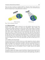
Climate change is a topic that has been widely discussed and debated over recent decades.
Scientists have reached a general agreement that the lower atmosphere and the Earth’s
surface are definitely getting warmer. The Intergovernmental Panel on Climate Change
(IPCC) reported that a gradual but accelerating increase of atmospheric greenhouse gases
has occurred since 1750 as result of human activities and among the anthropogenic
greenhouse gases, CO
2
is the most important. The global atmospheric concentration of CO
2

has increased from a pre-industrial value of about 280 ppm to 379 ppm in 2005 (Alley et al.,
2007). Temperature has risen by about 0.3-0.6
o
C since the late 19
th
century. If CO
2

emissions
were maintained at 1994 levels, its concentration would increase to about 550 ppm by the
end of the 21
st
century (Chakraborty et al., 2000). Thailand is a member of the United Nation
Framework Convention on Climate Change (UNFCCC), which is negotiated by the nations
of the world in June 1992 (Michaelowa and Rolfe, 2001). The targets of the UNFCCC is to
reducing CO
2
emissions from the rate reported for 1990 during the five-year period from
2008 - 2012. This agreement is called the Kyoto Protocol which Thailand has ratified since
August 28, 2002. There are two alternatives to reduce CO
2
, these include decreasing fossil
fuel consumption and increasing carbon sink through forestry activities. According to
Article 3.3 of the agreed Kyoto Protocol, some CO
2
sources and sinks of forests shall be used
to meet the commitments (UNFCCC, 1997). The sources and sinks to be used were
measured as verifiable changes in carbon stocks in each commitment period (Terakunpisut
et al., 2007; Forest research, 2011).
Forestry sectors are known as an important natural brake on climate change since they play
an important role in the global both as a carbon sink and source because of their large
biomass per unit area of land (Gibbs et al., 2007). The carbon in forests originates from the
atmosphere and is accumulated in terms of the organic matter of soil and trees, and it
continuously cycles between forests and the atmosphere through the decomposition of dead
organic matter (Alexandrove, 2007). Thus, changing carbon stocks in forests can affect the
amount of carbon in the atmosphere. If more carbon accumulates in forest through

Biomass and Remote Sensing of Biomass


200
photosynthetic process, the forest will be a sink of atmospheric carbon. If the carbon stocks
in forests decrease and release carbon into the atmosphere, the forests will become a source
of atmospheric carbon. The carbon stocks of forests can change in two ways, on the one
hand as a result of changes in forest area and on the other hand as a result of changes in
carbon stocks on the existing forest area. Broadmeadow and Matthews (2003) report that
approximately 1.6 GtC per year have released into the atmosphere as CO
2
from
deforestation during 1990s, but at the same time forest ecosystems is believed to have
absorbed between 2 – 3 GtC per year.
Tropical forests have an importan role for carbon sequestration in a much higher quantity
than any other biome (Gorte, 2009) and also as a main carbon source to the atmoshere in
areas that have undergone deforestation or unsustainable management (Malhi et al., 2006).
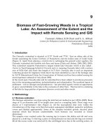
The amount of carbon storage in the world’s tropical forests which cover 17.6 x 10
6
km
2
are
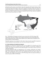
approximately 4.28 x 1011 tonne C in vegetation and soils (Lasco, 2002). Figure 1 shows the
total world’s tropical forests. In Asia, tropical forests are accounted for about 15.3 per cent
in the world (UNCTAD Secretariat, n.d.). However, these forest ecosystems are facing the
problem from deforestation and forest degradation in the tropics and Southeast Asia has
been no exception. Lasco (2002) indicates that in 1990 deforestation rate in Southeast Asia
was around 2.6x106 ha/ year. In addition there is liitle information on the carbon
sequestration in natural forest ecosystems in Southeast Asia. To understand carbon sources
and sinks, it is essential to estimate the biomass for these forests. Thus, the aim of this study
was to estimate and compare the aboveground biomass and carbon stock between primary
forest and secondary forest in the area of Khao Yai National Park.

2. Materials and methods
2.1 Study areas
This study was carried out at
Khao Yai National Park. It covers a large complex area in
Nakhon Ratchasima, Saraburi, Prachinburi and Nakhon Nayok Provinces. This National


Fig. 1. The distribution of the world’s tropical forest area in 2000 from UNCTAD Secretariat
(n.d.)
A Comparative Study of Carbon Sequestration Potential
in Aboveground Biomass in Primary Forest and Secondary Forest, Khao Yai National Park

201
Park is also part of the Dong Phaya Yen . The Dong Phayayen-Khao Yai Forest Complex is
an important pool of biodiversity and complex terresstrial habitats not only in region, but
also at global level. It was granted as a UNESCO Natural World Heritage Site on 14 July
2005 (Kekule, 2009). The climatological data was recieved from Khao Yai station,
Department of Meteorology provied 25 years from 1982 – 2006. The annual temperature in
the area varied from 30 - 33
o
C and the area recieved the annual mean precipitation of
1,123.48 ± 165.08 mm. The selected study areas were carried out in Nakhon Ratchasima
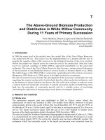
Province as shown in Figure 2. The sites were selected based on anthropogenic disturbance.
The primary forest was classified as non or least disturbed forested area and the main area
characteristic was classified as the tropical rain forest. On the other hand, the secondary
forest was disturbed from anthropogenic activities in the past and described as dry
evergreen and mixed deciduous forest types. All sampling plots were in the permanent plot
of Professor Emeritus Warren Y. Brockelman under the project : foraging and ranging
behavior of gibbons in Khao Yai National Park.



(a) The sampling plot in the primary forest (b) The sampling plot in the secondary forest
Fig. 2. The study sites in Khao Yai National Park
2.2 Data collection and analysis
A randomly 1 ha sampling plot (100 m x 100 m) in each forest type was established. To
reveal the tree composition and biomass, all live trees with a diameter ≥ 4.5 cm were
recorded. The diameter was measured at breast height (DBH, 1.3 m height from the ground)
to estimate biomass and the size class distribution of trees as well as species diversity in a
sampling plot. All supported botanical data were represented by the species in terms of
taxonomic classification identifie into Genera or Species, providing both local and scientific
names by Aunttara Na-Thalang, a researcher at BIOTEC central research unit and a co-
researcher of this project. In case of irregularities of trunk tree, the measurement was taken
at the nearest lower point where the stem was cylindrical, or above the buttresses on large
trunks. DBH was measured by used of diameter tape. Trees with multiple stems connected
near the ground were counted as single individuals and bole circumference was measured
separately. Tree height was recored by using a measuring pole. Figure 3 displayed primary
data record and field measurement.

Biomass and Remote Sensing of Biomass

202

(a) Trees ≥ 4.5 cmwere
measured
(b) DBH was measured above
the buttress root
(c) Tree height was recorded
Fig. 3. Field measurement
3. Data analysis
3.1 Species diversity and Important Value Index (IVI)

It was widely believe that species diversty related to the level of disturbance (Mackey and
Currie, 2001). Thus, species diversity was evaluated by using the Shannon – Wiener index
method (see Equation 1) in this study to compare between primary forest and secondary
forest. It was assumed that all species represented in the sampling plot were randomly
sampled. In this method, the proportion of number of individuals of a species to the overall
number of individuals in the sample plots was used to express the diversity of species in the
studied ecosystem (Krebs, 1999).

 
2
1
´ log
s
ii
i
Hpp



(1)
Where:
´Index of species diversit
y
H 

s Species number in the sample





i
 Proportional abundance of the th species n /N
i
pi
To investigate the structural role of tree in the sampling plots, the importance value index
(IVI) of each species was calculated using the percentage of relative abundance (R.A.),
relative dominance (R.D.) and relative frequency (RF) (see Equation 2)
I.V. R.A. R.D. R.F

……Whittaker (1970) (2)
Where:
A Comparative Study of Carbon Sequestration Potential
in Aboveground Biomass in Primary Forest and Secondary Forest, Khao Yai National Park

203
I.V. Important value index of each species


total number of each speciesx 100
R.A. Relative abundance
total nuber of all species

basal area of each species x 100
R.D. Relative dominance
basal area of all species

chance to find each speciesx 100
R.F. Relative frequency
chance to find all of species


To test the significance of the difference between categories, one way analysis of variance
(ANOVA) was carried out using the SPSS Statistics 17.0 software. Data on species
distribution in two forest types were analyzed by correspondence analysis using the same
software.
We used correspondence analysis (CA) as the ordination method to examine the
differences in the distribution of tree species
using the same software.
3.2 Aboveground biomass and carbon sequestration
To estimate aboveground biomass in the study areas by non – destructive methods, we had
to collect data such as diameter at breast height (DBH) and height of all trees. SILVIC
Program was used to predict the mean total tree height in the sampling plots. It was
developed from the relationship between DBH and tree height (Ht) by hyperbolic equation
(see Equation 3) or D – H curve (Ogawa, Yoda and Kira, 1961). Forty trees in different sizes
in the sampling plots were observed to analyse their height and DBH relationships. Ogawa
(1969) showed that H was approximately equal to one for most mature forests. Assuming
that h equaled one, the other coefficients, A and H* for each stand were calculated by using
the non – linear least square method. These constant values were used to predict tree height
in this study.


h
t
1/ H 1 /A DBH 1/ H* (3)
Where


Ht hei
g
ht of tree m



DBH diameter at breast hei
g
ht cm
A, h, H * constant
The next step was the aboveground biomass evaluation by non-destructive assessments. The
biomass regression equations on the basis of DBH and Ht which derived from in tropical
forests were applied for calculating the aboveground biomass and the size class analysis will
evaluate the status of forest ecosystem. The primary forest used the equation developed by
Tsutsumi et al. (1983) (see Equation 4) and the equation developed by Ogawa et al. (1965)
was used for the secondary forest (see Equation 5).

Stem (WS) = 0.0509*(D
2
H)
0.919
(4)
Branch (WB) = 0.00893*(D
2
H)
0.977

Biomass and Remote Sensing of Biomass

204
Leaf (WL) = 0.0140*(D
2
H)
0.669
and

Stem (WS) = 0.0396*(D
2
H)
0.9326
(5)
Branch (WB) = 0.003487*(D
2
H)
1.027
Leaf (WL) = ((28.0/ WS + WB) + 0.025)
-1
Where
Ws = stem mass
(kg/ individual tree)
Wb = branches mass
(kg/ individual tree)
Wl = leaf mass
(kg/ individual tree)
Ht = height of tree (m)
DBH = diameter at breast height (cm)
Total carbon content was estimated from aboveground biomass by converted from biomass
to carbon stock. From the reports (Atjay et al., 1979; Brown & Lugo, 1982; Iverson et al., 1994;
Dixon et al., 1994; Cannell & Milne, 1995 and Terakunpisut et al., 2007), carbon content
would be about fifty percent of the amount of aboveground biomass. To compare the
potential of carbon sequestration between primary forest and secondary forest, frequency
distribution of total aboveground biomass in a range of DBH size classes were considered to
assess the potential of the forests across their size classes and age.
4. Results and discussion
4.1 Species diversity
Across sampling sites, tree species varried with forest types. Primary forest had greater

species richness (75 species/ ha) than secondary forest (47 species/ ha). It probably implied
that the study site in primary forest was more complexity in a community and species
interaction. Since number of species compositions indicated the degrees of energy transfer
through foodweb. In this case, the level of energy transfer in primary forest was stronger
than secondary forest in order to support the higher total number of individuals of all
species. This meant that the productivity in primary forest was also higher than another. In
addition, the greater number of species compositions were most in ecosystems that have
long time evolution, because organisms may develop mechanisms to conserve or more
efficiently acquire any of the other limiting resources by certain physical or abiotic factors of
the environment such as temperature, precipitation, light and soil.
From the species diversity (H´) measurement, The results showed that the overall plant
species diversity of primary forest was higher than secondary forest, with the Shannon-
Wiener indexes being 3.46 and 2.03 respectively. In practical, species diversity has been used
to indicate the stability of the ecosystem. It meant that the high species diversity can exist in
the spatially heterogeneous environment where the disturbances influence to the species in
different degree. The species diversity index values measured and calculated from different
forest ecosystems in Thailand had been listed and compared with this study as shown in
Table 1. The species diversity values in primary forest and secondary forest were not much
different from others study. The main conclusion was clearly demonstrated that the highest
species diversity was from primary forest (tropical rain forest) because there were rich in
A Comparative Study of Carbon Sequestration Potential
in Aboveground Biomass in Primary Forest and Secondary Forest, Khao Yai National Park

205
resource such as diverse of habitat types and a large extent on food available in the tropical
rain forest more than in other forest types.

Forest ecosystem
Shannon – Wiener diversity
index

References
The primary forest
The secondary forest
3.46
2.03
This study
Tropical rain forest 3.48 - 3.52 Terakunpisut et al., 2007
Dry evergreen forest
3.62
3.5 – 4.9
Terakunpisut et al., 2007
Sahunalu et al., 1979
Mixed deciduous forest
3.09
3.5 – 3.9
Terakunpisut et al., 2007
Sahunalu et al., 1979
Table 1. A comparison of species diversity index under different forest ecosystems in
Thailand among this study and the others.
This study also identified the dominant species according to the important value index (IVI).
The result represented in Figure 4, which ranked from the highest value to lower value. The
result indicated that common species in the primary forest were Ardisia nervosa (127 tree/
ha, IVI = 56.08) followed by Mastixia pentandra, Gonocaryum lobbianum, Dipterocarpus gracilis,
Cinnamomum subavenium and Aglaia elaeagnoidea. The contribution of the dominant species in
the secondary forest was Schima wallichii (505 trees/ ha, IVI = 71.94) and 2 co-dominant
species were Machilus odoratissima and Eurya nitida.


Fig. 4. Important value index of tree species (DBH ≥ 4.5 cm) in the primary forest and the
secondary forest


Biomass and Remote Sensing of Biomass

206
The correspondence analysis revealed the pattern of the species distribution tree
distribution in the study areas (see Figure 5). A correspondence map displayed two of the
dimensions to relate the distribution of tree species with forest types. It showed that some
plant species had high potential distribution. Thus, there were overlapped in their
distribution between the different forest types. For example, Aquilaria crassna, Bridelia
insulana, C. subavenium, Cleistocalyx operculatus, D. gracilis, Eurya nitida, Garcinia benthamii, G.
lobbianum, Helicia formosana, Ilex chevalieri, Litsea umbellata, M. pantandra, Phoebe lanceolata,
Syzygium grande, S. siamensis and S. Syzygiodes occurred in both forest types and the pattern
indicated links to both forests. Because of the similarity of climate such as annual
precipitation and annual temperature, the species compositions of each forest type had
features in common and only a few rare species were specific to a single forest type. The
analysis of variance showed that tree species did not significantly differ across the two forest
types in terms of species richness, F (1, 120) = 2.328, p = 0.130. This was due to several
species were found in both forests.


Fig. 5. Species distribution and forest types. Tree compositions in both forests were not
significantly different across groups, F (1, 120) = 2.328, p = 0.130
Figure 6 showed the DBH size class distribution on two sampling plots. The density of
plants with DBH ≥ 4.5 cm in secondary forest was 1,249 trees/ ha due to lots of small tree
sizes. While tree density in primary forest was only 919 trees/ ha since the main tree size
class in this area was medium to large tree sizes at DBH > 40 – 60 cm and 60 – 80 cm. It was
cler that the frequency distribution curves of DBH were all L- shaped in both forests. The
density of trees was the highest at the left end of the graph and decreased afterward. Up to
> 20 – 40 cm, the distribution curves of primary forest and secondary forest were similar,
A Comparative Study of Carbon Sequestration Potential

in Aboveground Biomass in Primary Forest and Secondary Forest, Khao Yai National Park

207
although the amount of trees in secondary forest were much higher, especially in DBH size
class ≥ 4.5 – 20 cm. The main differences between primary forest and secondary forest were
in the number of trees in medium size class at DBH > 40 – 60 cm and > 60 – 80 cm which
were greater amount in primary forest. The analysis of variance showed that there was
significant difference of tree density between primary forest and secondary forest, F (1, 120)
= 4.393, p = 0.038.


Fig. 6. A trend of tree density distribution in different DBH size classes
4.2 Aboveground biomass and carbon sequestration
Aboveground biomass distribution and carbon storage in different DBH size classes were
compared between primary forest and secondaryforest in Khao Yai National Park (see
Figure 7). It was remarkable that total aboveground biomass accumulation in primary forest
(684.76 tonne/ ha) was higher than seconday forest (198.20 tonne/ ha). Although the
number of trees were significantly greater in secondary forest, but the highest tree density
were in the group of small tree size classes at DBH ≥ 4.5 – 20 and 20 – 40 cm which had
lowest individual volume and biomass. On the other hand, the most aboveground biomass
accumulation was found in big trees of size class at > 60 – 80, > 80 –100 and > 100 cm that
were dominant tree groups in primary forest. Because these trees were highest stem volume
and large diameter, although they were the smallest group of tree densities. The analysis of
variance revealed a significant difference in terms of median total aboveground biomass
between primary forest and secondaryforest, F (1, 3046) = 29.189, p = 0.000.
In comparison with other tropical forests, the range of aboveground biomass in this study
both areas were similar (see Table 2). The result in Primary forest was compared to tropical
rain forest, while data in secondary forest was compared with the biomass in dry evergreen
forest and mixed deciduous forest.


Biomass and Remote Sensing of Biomass

208

Fig. 7. Frequency distribution of total aboveground biomass in a range of DBH size classes
between the primary forest and the secondary forest

Forest ecosystem
Aboveground biomass
(tonne/ ha)
References
The primary forest
Tropical rain forest
684.76
509.00
This study
Yamakura et al., 1986

The secondary forest
Dry evergreen forest
Dry evergreen forest
Mixed deciduous forest

198.20
73.06 - 173.10
140.58
96.28
This study
Mani and Parthasarathy, 2007
Terakunpisut et al., 2007

Terakunpisut et al., 2007

Table 2. A comparison of total aboveground biomass in this study and the others.
The percentage data of tree density and carbon sequestration were presented in Table 3. The
total carbon sequestration in primary forest and secondary forest were equal to 342 and 99.10
tonne C/ ha, respectively. The results showed that the distribution of DBH size classes and the
total carbon storage in each size class varied between the forest types. About 80 per cent of
the carbon stock was presented in DBH size class at ≥ 4.5 – 20 cm and > 20 – 40 cm in
secondary forest but contributed only 20 per cent of total carbon stock in primary forest. The
carbon storage was highest in DBH size class at > 60 – 80 cm and > 80 – 100 cm in primary
forest.
However, the highest potential size class to sequester CO
2
from the atmosphere in primary
forest and secondary forest were DBH size class at > 60 – 80 cm and > 20 – 40 cm,
respectively. Since number of trees in these size classes were lower than other, but the
A Comparative Study of Carbon Sequestration Potential
in Aboveground Biomass in Primary Forest and Secondary Forest, Khao Yai National Park

209
amount of carbon storage were greater than other groups which had higher tree density. For
example, in secondary forest; trees in the size class at ≥ 4.5 – 20 cm were five times more tree
density than trees in the size class at > 20 – 40 cm, but the amount of carbon storage were
similar. Likewise primary forest, trees in the size class at > 60 – 80 cm were found only 0.44
per cent, but the amount of carbon storage was nearly four times of trees in the size class at
≥ 4.5 – 20 cm.

size class The primary forest The secondary forest
(DBH, cm) Tree density (℅) Carbon stock (℅) Tree density (℅) Carbon stock (℅)
≥ 4.5 - 20 76.20 6.93 85.30 38.18

> 20 - 40
20.00 13.43
14.37 39.96
> 40 - 60 3.04 6.37 0.19 1.48
> 60 - 80 0.44 26.73
0.05 0.62
> 80 - 100 0.33 46.53 - -
> 100 - - 0.09 19.75
Table 3. A comparison of the percentage of tree density and carbon sequestration potential
between the primary forest and the secondary forest
In summary, the distribution pattern of aboveground biomass had been related to past
disturbance history the forests. Total aboveground biomass in the primary forest was about
triple that of the secondary forest. However, both study areas had high carbon sequestration
potential in the future due to presence of large number of trees belonging to small DBH size
classes. These trees in size class at ≥ 4.5 – 20 cm were in the youth phase and their growth
rate was accelerating to reach maturity. It meant that at the present these smaller trees are
not the highest carbon sequestration potential, but in the near future they can sequester CO
2

from the atmosphere through photosynthesis to form their structure till senescent phase.
Broadmeadow and Matthews (2003) suggested the option to reserve carbon in the forests by
minimal intervention, with a gradual long – term increase in carbon stocks.
5. Conclusions
The number of tree species occurring on the sample area in the primary forest and the
secondary forest were 75 and 47 species, respectively. To conclude the correspondence
analysis and ANOVA, it was found that there were many species in common between
primary forest and secondary forest. So each forest type had not a distinctive of species
distribution. From the results, it was found that the tree density was counted in the
secondary forest as 2,129 trees/ ha due to lots of saplings and small trees, while the tree
density in the primary forest was found only 919 trees/ ha since the main tree size class in

this area was medium to large tree size at > 60 – 80 cm.
The primary forest and secondary forest of Khao Yai National Park had carbon stocks 342.29
and 99.10 tonne C/ ha, respectively. The total aboveground carbonstorage in the primary
forest was significantly greater than the secondary forest. Although the young trees
belonging to the size class at DBH ≥ 4.5 - 20 cm dominated both forests in terms of tree
density, the carbon sequestration potential was greater in the size class at DBH > 20 - 40 cm
in secondary forest and in the size class at DBH > 60 - 80 cm in primary forest. Both forests
were very important for carbon sequestration because there were typically high carbon

Biomass and Remote Sensing of Biomass

210
stocks. Moreover, the result also implied that the potential was considerably high to
sequester carbon in both forest areas in the near future due to lots of small trees in the areas.
We hope that the results of this study on aboveground biomass and carbon sequestration
will be useful to conserve these forest areas under sustainable management.
6. Acknowledgements
The authors express their sincere gratitude to Kasetsart University Research and
Development Institute (KURDI) for financial support of this project and wish to thank
Kasetsart University for support in publishing. The authors also thank the Biodiversity
Research and Training Program (BRT) to support young sciencetists. The authors are
thankful to Professor Emeritus Warren Y. Brockelman, for his support valuable data use in
this article and giving permission to carry out field work in the permanent plot under the
project: foraging and ranging behavior of gibbons in Khao Yai National Park. The author
also thanks the staff of Professor Emeritus Warren Y. Brockelman’s project and a team of
undergraduade students from the Faculty of Liberal Arts and Science, Kasetsart University
for help in the field survey. A big thank you also goes out to Dr. Taeng-on Prommi, a
lecturer at Faculty of Liberal Arts and Science for help in the application process of
publishing grant. Also thank Megan Combs for always improving the language of this
paper.

7. References
Alexandrove, G.A. (2007). Carbon Stock Growth in a Forest Stand: the Power of Age, Carbon
Balance and Management, Vol. 2 (4), pp. 1 – 5.
Alley, R., Berntsen, T., Bindoff, N.L., Chen, Z., Chidthaisong, A., Friedlingstein, P., Gregory,
J., Hegerl, G., Heimann, M., Hewitson, B., Hoskins, B., Joos, F., Jouzel, J., Kattsov,
V., Lohmann, U., Manning, M., Matsuno, T., Molina, M., Nicholis, N., Overpeck, J.,
Qin, D., Raga, G., Ramaswamy, V., Ren, J., Rusticucci, M., Solomon, S., Somerville,
R., Stocker, T.F., Stott, P., Stouffer, R.J., Whetton, P., Wood, R.A. & Wratt, D. (2007).
The Fourth Assessment Report of the Intergovernmental Panel on Climate Change: Climate
Change 2007: the Physical Science Basis, Geneva, Switzerland, Intergovernmental
Panel on Climate Change.
Atjay, G.L., Ketner, P. & Duvignead, P. (1979). Terrestrial Primary Production and
Phytomass. In B. Bolin, E.T. Degens, & S. Kempe, (Eds.), The Global Carbon Cycle,
Wiley and Sons, New York, pp. 129 – 182,
Broadmeadow, M. & Matthews, R. (2003). Forests, Carbon, and Climate Change: the UK
Contribution, Information Note, June 2003. Available from

Brown, S. & Lugo, A.E. (1982). The Storage and Production of Organic Matter in Tropical
Forests and Their Role in the Global Carbon Cycle, Biotropica Vol 14, pp. 161 – 187.
Cannell, M.G.R. & Milne, R. (1995). Carbon pools and sequestration in forest ecosystems in
Britain, Forestry Vol 68, pp. 361 – 378.
Chakraborty, S., Tiedemann, A.V. & Teng, P.S. (2000). Climate Change: Potential Impact on
Plant Diseases, Environmental Pollution Vol.108, pp. 317-326.
Dixon, R.K., Brown, S., Solomon, R.A., Trexler, M.C. & Wisniewski, J. (1994). Carbon Pools
and Flux of Global Forest Ecosystems, Science Vol 263, pp. 185 – 190.