Wind Energy Management Part 4 pdf
Bạn đang xem bản rút gọn của tài liệu. Xem và tải ngay bản đầy đủ của tài liệu tại đây (878.15 KB, 13 trang )
Wind Energy Management
30
Skov, H., Krogsgaard, J., Piper, W., Durinck, J. (2009). Anholt Offshore Wind Farm. Birds.
Report to EnergiNet.Dk. DHI.
Sokal, R.R. & Rohlf, J.F. (1981). Biometry: the principles and practice of statistics in bio-logical
research. 2nd ed., W. H. Freeman and Company, San Francisco.
Part 3
Power System Control
3
Technical Framework Conditions to
Integrate High Intermittent Renewable
Energy Feed-in in Germany
Harald Weber
1
, Christian Ziems
1
and Sebastian Meinke
2
1
Institute of Electrical Power Engineering
2
Department of Technical Thermodynamics
University of Rostock
Germany
1. Introduction
The first part of this chapter gives a short overview about the general problems of
integration. Therefore a control theory based description of the basic fundamentals of the
power system control concepts is given.
The second part of the chapter concentrates on the technical framework conditions of
conventional power plants to follow the intermittent power feed-in because as long as no
large-scale storage systems are available these conventional power plants will be necessary
to integrate the renewable energy at least for the next 20 years. Therefore different methods
and tools to analyze and simulate the power plant scheduling and to determine the
additional life time consumption of highly stressed components of fossil fueled power
plants will be presented and illustrated by different scenarios.
2. German ambitions for renewable energy until 2050
In Germany the existing electrical generation system is going to be essentially influenced
due to the continuously increasing influence of intermittent renewable energy sources.
Because of the massive expansion of the total number of wind turbines, especially in the
northern part of Germany within the last years, wind power now plays the most important
role concerning the renewable energy sources in Germany.
At the end of 2010 the installed capacity of wind turbines amounted to more than 27.2 GW.
Besides the photovoltaic capacities are increasing so fast, that at the end of 2010 there was
more than 17.4 GW of installed capacity for photovoltaic systems. In the photovoltaic sector
this was an increase of about 80 % compared to 2009.
Despite of a stepwise reduction of the legal refunds for the electrical energy produced by
photovoltaic systems and wind turbines in Germany within the next 10 years, current
predictions yield to about 50 GW of installed capacity for photovoltaic systems and an
installed capacity of wind turbines of more than 51 GW in 2020. This means that there will
be probably more than 100 GW of wind and solar power generation installed in Germany by
the end of the decade. Therefore the share of electrical energy produced by these two
Wind Energy Management
34
renewable sources could increase from 8.6 % in 2010 to more than 35 % in 2020 of the
German electrical net energy consumption.
In regard to a peak load of 85 GW and an off-peak load of only 45 GW there will be new
challenges to integrate such a high intermittent power feed-in into the existing electrical
generation system. Until now there are only the fossil and nuclear power plants available to
balance the renewable energy production and to follow the wind and solar power
production in a complementary way. But due to the increasing fraction of intermittent
renewable energy sources within the generation system the number of available
synchronized conventional power plant generators will be reduced continuously especially
in periods with high renewable power feed-in. Since the system stability depends on the
availability of flexible power stations, sufficient spinning reserves and certain system inertia,
the robustness of the electrical power system will reduced towards suddenly appearing
disturbances of the power balance.
Due to the limited fossil and nuclear resources that we use today and the high carbon
dioxide emissions and nuclear waste production to produce more than 80 % of the German
electrical energy, Germany has to exploit new energy sources that are available in an
unlimited way. Therefore in the 21
st
century the renewable energies will become the most
important field of research in several domains of technology. Wind and solar energy are
available nearly everywhere in Germany. But it will depend on several economical
boundary conditions which kind of technology will be the best to gain an efficient access to
this unlimited energy supply.
Of course in regard to the relevance of solar energy it would be the most efficient way to
generate the electricity where the solar energy supply is naturally the highest. But
unfortunately these regions are often far away from the areas with the high population and
consumption density. For example it would be possible to cover the total worldwide energy
consumption by just covering a very small fraction of the desert areas like the Sahara in
North Africa, but a very powerful transportation system for electrical energy is needed that
has to consist of various high voltage transmission lines that can deliver the energy to the
consumers. In Europe for example the consumers are several thousand kilometers away
from the desert areas and of course Europe is separated from the continent of Africa by the
Mediterranean Sea. So it would be necessary to use cable systems to connect this
intercontinental sea distance which are very cost-intensive compared to overhead lines.
These new transmission line systems will cause very high capital expenditures that can’t be
raised in the near-term future. This funding, on the one hand for the transmission line
systems and of course on the other hand for the solar generators like Concentrated Solar
Power (CSP) stations or photovoltaic (PV) systems, has to be invested in the long-term
future. Although in Europe there is a first ambitious entrepreneurship called Desertec, that
proposed to it selves that it could be possible to build up such a renewable solar and wind
generation system in North Africa within the next decades, earliest in 2050 almost 15 % of
the electrical energy consumption of entire Europe could be covered. But in regard to the
security of supply it has to be mentioned that there is always a certain risk in dependence to
other countries especially when the political systems are not stable in these countries.
So to fulfill the German goals and to be less dependent from foreign political issues it is
necessary to use the renewable energy sources that are available on the German land and
sea area to increase the fraction of renewable energy in the electrical energy system from
18 % today up to 40 % until 2020 and up to 80 % until 2050.
The potential especially for wind energy is very high in Germany. Naturally the solar
energy potentials aren’t as high as in southern Europe or North Africa but nevertheless it is
still worthwhile to exploit this renewable energy source with photovoltaic systems. In
Technical Framework Conditions to Integrate
High Intermittent Renewable Energy Feed-in in Germany
35
Germany hydro power is already exploited to a great extent and biomass and geothermal
energy aren’t capable to contribute big proportions of the energy consumption. Therefore
only the intermittent energy sources like wind and photovoltaic power can be used to
deliver a high proportion of the total energy demand.
But unfortunately these two energy sources have a very disadvantageous characteristic.
They occur in an intermittent way and they aren’t reliable. Furthermore the energy supply
of wind and solar generators do not correlate to the overall energy consumption. From the
consumers point of view this makes it impossible to operate an electrical generation system
without any backup power plants that are supplied by big storage systems. Besides these
backup power stations are necessary to ensure the safety of supply at any time even when
the system is disturbed by suddenly appearing technical outages of any electrical equipment
of the generation system. Moreover fast reacting generators are essentially needed especially
when the wind and solar energy occurrence is decreasing due to changing meteorological
conditions.
3. The electrical generation system as a controlled system: frequency –
active power – control
To understand the fundamental problems of the integration of intermittent renewable
energy sources into the electrical generation system it is very important to understand the
control structure of the system. Therefore in the following subsections a more detailed
description of the electrical generation system, which is precisely a controlled system, will
be given.
Worldwide the electrical energy supply is operated with a three-phase network. Three-
phase rotary current is used instead of single phase Alternating Current (AC) because its
behavior towards the transmission of energy is similar to a rotating mechanical shaft which
is continuously delivering power. But this virtual “electrical shaft” is not emitting noise nor
is it necessary to lubricate it. From the powered generator shaft to the slowing down motor
shaft the three-phase rotating current network therefore behaves like a warped torsion shaft
under workload that rotates with 50 rotations per second. Hence the electrical switch- and
transformer-stations act like mechanical gearboxes that are connected to several distribution
shafts which are connected with the consumers. The consumer can use these distribution
shafts to perform mechanical work or to produce light or heat by the cause of friction. The
shafts are driven by different mechanical power drives which care for the n
T
=50 rotations
per second and provide the torque M
T
which is required for the delivered power P
T
according to:
2
TTTT T
PM M n
(1)
This torque is produced by turbines that are classed into thermal, gas fired and hydraulic.
To ensure a long life time of the power drives the rotational speed n
T
has to be kept as
constant as possible. Therefore only the torque M
T
can be adjusted which means more or
less steam, gas or water onto the turbine. The turbines consist of rotors which have an
inertia Θ. But a rotating mass is only able to change its rotational speed if the sum of
working torques is changed according to:
()
TTV
MM
(2)
Wind Energy Management
36
Here M
V
is the delivered load torque: If M
T
increases the system accelerates, if M
V
increases
the system slows down. The rate of acceleration or deceleration of the whole system is
significantly determined by the inertia Θ. Hence if the inertia would be reduced the
rotational speed change rate would increase, too.
To summarize this first part it can be outlined that if the mechanical system wouldn’t emit
noise and if it wouldn’t be necessary to lubricate the components, the energy supply
systems could be realized with pure mechanical components. To understand the frequency –
active power – control loop it is therefore sufficient to understand the controlled mechanical
energy supply system.
In control engineering usually per unit (p.u.) values are used for different physical values.
These per unit values are referenced to their nominal value. If furthermore is assumed that
the rotational speed n
T
and therefore Ω
T
isn’t changed noteworthy, equation (2) can be
constituted as:
()
NT T V
PP
(3)
If the nominal values P
G
and Ω
N
are introduced, equation (3) can be written as:
()
GTV
T
fpp
(4)
The values indexed with G stand for values referenced to the whole network. Here f is the
per unit system frequency or rotational speed. T
G
is called the acceleration time constant and
it is calculated by:
2
N
G
G
T
P
(4a)
The acceleration time constant, which is calculated by the inertia of the generators and
motors, commonly states how much time it takes from standstill to accelerate an inertia that
is driven by its nominal torque or power until the nominal rotational speed is reached.
Within the electrical energy system the inertia is of vital importance, since only the inertia is
able to stabilize the network frequency at an acceptable value in the first moment after a
disturbance of the power balance. Normally wind turbines are connected to the system via
frequency inverters and photovoltaic systems are always connected via DC/AC converters,
so they are mechanically and electrically decoupled from the system and can not increase
the acceleration time constant. Therefore it is has to be lined out that the acceleration time
constant is reduced if more and more wind turbines and photovoltaic panels are connected
to the system when at the same time the number of conventional power plant generators
with masses are displaced by these intermittent generators while the total nominal power
value of the whole system remains constant.
3.1 The primary control
With the use of the Laplace transform equation (4) can be stated according to:
1
()
EV
GG
G
fpp
sT
(5)
Technical Framework Conditions to Integrate
High Intermittent Renewable Energy Feed-in in Germany
37
The values indexed with G stand for values referenced to the whole network, index E for the
generation and V for the consumption. This equation of motion is the basis of the control
orientated modelling structure of the primary control of a total network shown in Fig. 1.
Here the frequency f is stated as the deviation from the desired network frequency that is
50 Hz in Europe. Furthermore the following assumption was made: All power plants and
consumers are connected to a single node network model; this means the transmission lines
or transmission shafts between them are neglected. Therefore only one network frequency
exists. The losses are allocated to the consumers. p
GE
describe the total power generation
and p
GV
the total power consumption in per unit values. With this kind of model the whole
European generation system of the ENTSO-E from Portugal to Poland and Denmark to
Turkey with a total nominal power of P
G
= 300 GW can be described.
Due to the dependency of the power consumption of motors on the network frequency the
real absorbed power p
GV
is corrected by the frequency dependent change of power Δp
GVf
according to:
1
f
V
GV
G
pf
(6)
This behaviour is called the consumer self-controlling effect which is expressed by σ
GV
. The
mean value for this value is 200 % in Germany. Therefore the consumers itself acts like a
control loop because they reduce their power consumption if the frequency decreases and
they increase their power consumption if the frequency increases. Hence in Fig. 1 the
magenta-hued total consumer has three single paths:
1.
The actual operating point of the consumed power
2.
The always occurring disturbance of the system because of consumer re- and
disconnections from the system
3.
The frequency dependent power consumption of the motoric consumers
The operating point “consumed power” is the forecasted power demand of the total
network at a certain hour of the day. All deviations from this value result in the disturbance
signal “consumer re- and disconnection”. The operating point “consumed power” has to be
covered by the existing power plants. In Fig. 1 this is symbolized by the “scheduled power”.
The operating point “secondary control power” will be described later. For now it can be
assumed to be zero.
If now is assumed that only the consumer self-controlling effect would take effect, the
deviation of the network frequency from the nominal value of 50 Hz would increase to a
non-permissible extent. In Fig. 2 this deviation is illustrated by the green line for a step
disturbance of the consumed power of 1 % of the nominal power. For the European
network with a nominal power of P
G
= 300 GW this is equal to a disturbance of 3 GW. The
primary control is designed to handle such a disturbance at the maximum and to
compensate the power deficit completely. This maximum disturbance is equal to the outage
of two French nuclear reactors of the nuclear power plant Tricastin. As withdrawn in Fig. 2
the frequency deviation amounts to Δf = -0.02 pu = -2 % or -1 Hz. In the case of such a high
frequency deviation first consumers would be automatically disconnected from the system
to ensure the safety of supply and to protect electrical components.
Wind Energy Management
38
Fig. 1. Control oriented scheme of the primary control
Technical Framework Conditions to Integrate
High Intermittent Renewable Energy Feed-in in Germany
39
0 10 20 30 40 50 60 70 80 90 100
-0.02
-0.018
-0.016
-0.014
-0.012
-0.01
-0.008
-0.006
-0.004
-0.002
0
delta f in pu
Time in s
df(t) with PP
df(t) without PP
Fig. 2. Frequency deviation in pu while Δp
GV
= +1 %
The step-shaped disturbance of the consumed power of 1 % has to be covered at any time. In
Fig. 3 the different types of power are shown that cover this additional consumed power:
The blue line shows the reduction of the real consumed power due to the consumer self-
controlling effect according to equation (6), the green line shows the accelerating power that
is delivered by the inertia of each rotating mass that slows down corresponding to equation
(7). As outlined by this graph in the first moment the required power is delivered by the
accelerating power that is provided by the decelerating rotating masses and later by the
consumer self-controlling effect which is reacting due to the decreasing frequency.
acc
GG
p
T
f
(7)
In the future the electrical generation system will be characterized by inertia-free energy
converters like frequency inverter controlled wind turbines and photovoltaic panels, so the
accelerating power has to be generated synthetically with power electronics to safe the grid
control and to ensure the system stability any longer.
In the control orientated structure of Fig. 1 the controller “primary controller” and the
manipulated variable “primary control power” are shown. This primary reserve power has
to be reserved in all power plants that are connected to the system. Due to this primary
reserve power the frequency deviation is kept in an acceptable tolerance range which is
illustrated by the blue line in Fig. 2. Here the frequency deviation remains within -200 mHz
in regard to a steady state evaluation if a σ
P
of 14 % is assumed.
Wind Energy Management
40
0 10 20 30 40 50 60 70 80 90 100
-6
-4
-2
0
2
4
6
8
10
12
14
x 10
-3
Tim e in s
pGVf without PP
pGacc without PP
Fig. 3. Disturbance of the power balance covered by accelerating power and the consumer
self-controlling effect
In this context in Fig. 4 the accelerating power is shown again. Here now the primary
control (red line) almost entirely takes over the disturbance slightly supported by the
consumer self-controlling effect. This transition process proceeds oscillating as well as the
corresponding frequency change. The related power plant model was simplified to two
PT1-elements with the time constants T
K1
= 0,8 s and T
K2
= 6 s.
In the future as mentioned before the acceleration time constant T
G
will be reduced due to
the increasing amount of renewable generation from wind and photovolaics because of the
loss of inertia. In Fig. 5 is shown the effect of a reduced inertia. Therefore the network
acceleration time constant is reduced from 12 s to 6 s and then to 2 s. As illustrated in the
three lines of diagrams at the beginning the frequency deviation increases, the network
behaviour gets “softer”, although the disturbance remains constant in all three cases. This
behaviour will continue until the primary controller stability is lost completely in the third
scenario due to the lack of sufficient inertia.
3.2 The secondary control
The operating point “secondary control” in Fig. 1 remained zero in case of the
aforementioned primary control action which acts in the domain of seconds. This caused a
remaining steady state deviation of the frequency as shown in Fig. 2. This deviation is now
corrected by the secondary control within the domain of minutes whereby this process has
to be finished after 15 minutes.
Technical Framework Conditions to Integrate
High Intermittent Renewable Energy Feed-in in Germany
41
0 10 20 30 40 50 60 70 80 90 100
-6
-4
-2
0
2
4
6
8
10
12
14
x 10
-3
Time in s
pGVf with PP
pGacc with PP
pGP with PP
Fig. 4. Disturbance of the power balance covered by accelerating power, the consumer self-
controlling effect and the primary control
0 20 40 60 80 100
-5
0
5
x 10
-3
delta f in pu
Time i n s
Freq(TN=12,Tk=3,Tk1=.8)
0 20 40 60 80 100
0
0.005
0.01
0.015
0.02
pGP in pu
Time i n s
0 0.005 0.01 0.015 0.02
-4
-3
-2
-1
0
1
x 10
-3
delta f in pu
pGP in pu
0 20 40 60 80 100
-5
0
5
x 10
-3
delta f in pu
Time i n s
Freq(TN=6,Tk=3,Tk1=.8)
0 20 40 60 80 100
0
0.005
0.01
0.015
0.02
pGP in pu
Time i n s
0 0.005 0.01 0.015 0.02
-4
-3
-2
-1
0
1
x 10
-3
delta f in pu
pGP in pu
0 20 40 60 80 100
-5
0
5
x 10
-3
delta f in pu
Time i n s
Freq(TN=2,Tk=3,Tk1=.8)
0 20 40 60 80 100
0
0.005
0.01
0.015
0.02
pGP in pu
Time i n s
0 0.005 0.01 0.015 0.02
-4
-3
-2
-1
0
1
x 10
-3
delta f in pu
pGP in pu
Fig. 5. Effect of a reduced acceleration time constant due to reduced inertia onto the primary
controller stability
Wind Energy Management
42
Furthermore the secondary control has to determine in which control area of the system the
disturbance occurred because only the disturbed control area should compensate the
disturbance. In this context it is important to consider the scheduled exchange power
between different control areas, too. The secondary control detects the disturbance by the
use of the Area Control Error (ACE). After the transient oscillation of the primary control
the ACE is zero in a non-disturbed control area and in the disturbed control area the ACE is
equal to the sum of the power balance (import positive, export negative). Basically the
following equation has to be fulfilled for every control area after the transient oscillation of
the primary control:
Zero = deviation of primary control power – deviation of exchange power -
disturbance power
In the case of a consumer reconnection the disturbance power is positive; in case of a
disconnection it is negative. If now the equation above is transposed it reads as follows:
disturbance power = -ACE = deviation of primary control power –
deviation of exchange power
or
AA
TT TT
ACE K
f
PoderACEK
f
P
(8)
The Area Control Error ACE of the secondary control reads as follows:
A
TT
ACE K
f
P
Here values with index T belong to the part-networks and index A for the exchange power.
By the estimation of the deviation of the primary control power and by measuring the
deviation of the exchange power the each time appearing disturbance power can be
determined. The coefficient K
T
given in MW/Hz necessary for this estimation is determined
by the measurement of the real network coefficient of the primary control of a part-network
Λ
T ,
whereas this coefficient is about Λ
G
= 20 GW/Hz for the whole ENTSO-E network in
non per unit values today. Generally for the total network it reads as follows:
1
N
GG G
GG
f
and
P
(9)
The inverse value of the network coefficient λ
G
is called the network statics σ
G
. The per unit
value of network coefficient λ
G
is calculated by the per unit values of the network
coefficients of the part-networks according to:
11
ii
i
i
TT
GT
ii
GGTG
PP
oder
PP
(10)
For the steady-state frequency deviation of the primary control of the total network in Fig. 1
in the case of steady-state considerations the deviation is calculated by:
V
GG
fp
(11)
σ
G
describes the statics of the total network including the self-controlling effect of all
consumers. Under consideration of this relation the control oriented block diagram shown