Power Quality Monitoring Analysis and Enhancement Part 6 docx
Bạn đang xem bản rút gọn của tài liệu. Xem và tải ngay bản đầy đủ của tài liệu tại đây (1.72 MB, 25 trang )
Power Quality – Monitoring, Analysis and Enhancement
112
2
22 2
1
2
0
,
imj
N
mn N
m
nmn
SjT H e e
NT NT
π
π
−
−
=
+
=
(18)
where n≠0 and H[n/NT] is the Fourier transform of time series.
The STFT transform limitation is the fixed window width, chosen a priori, for analysis of
nonstationary signals containing low-frequency and high-frequency components.
Consequently, the frequency-time resolution is fixed too and is difficult to analyze a
sinusoidal signal of low frequecy (for instance the signal from power supply network)
affected by a high frequency disturbance (for instance a transient phenomenon).
The wavelet transform limitations are: low resolution for low-frequency components, the
decomposition frequency bands are fixed, noise sensitivity.
The S transform is an extension of the wavelet transform resulted using a phase correction
which provides superior resolution.
Applying DST on a signal the result is a matrix within the rows are frequences and the
columns are time values.
5.1 Using the S-transform
To ilustrate the ability of the ST to detect, localize and quantify power quality disturbances
are considered two signals. First signal is afected by a voltage swell (low-frequency
components) and the second by an impulsive transient (high-frequency components).
Figure 11 shows the 3D ST plots for both signals. From the 3D plots can be observed the
amplitude variations of the frequency spectral components in the signals.
Fig. 11. S-transform 3D representation
Methodes of Power Quality Analysis
113
Figure 12 presents the ST of a clean signal and six types of power quality disturbances
(voltage sag, voltage swell, voltage interruption, voltage harmonics, impulsive transient and
oscillatory transient): a) the signal, b) the normalized time-frequency contour of ST, c) the
maximum of amplitude-time characteristic of S transform and d) the maximum of
amplitude-frequency characteristic of of S transform. From visual inspection of these plots
are obtained amplitude, frequency and time information in order to detect, localize and
classify the disturbance.
Power Quality – Monitoring, Analysis and Enhancement
114
Fig. 12. S-transform
Figure 12 shows that the maximum of amplitude-time characteristic of S transform is
constant for the clean signal and voltage harmonics and the maximum of amplitude-
frequency characteristic of S transform reflects the changes in frequency domain due the
presence of disturbances.
6. Impulsive transient characterization
The power quality disturbances that may occur in power supply networks are classified in
various categories (Dungan, 2004): transient phenomenons, short duration variations, long
duration variations, voltage imbalances, waveform distortions, power frequency variations
and flickers.
Transient phenomenons are sudden and short-duration change in the steady-state condition
of the voltage, current or both. These phenomenons are classified in two categories:
impulsive and oscillatory transient. The first category has exponential rise and falling fronts
and is characterized by magnitude, rise time (the time required for a signal to rise from 10%
to 90% of final value), decay time (the time until a signal is greater than ½ from its
magnitude) and its spectral content.
In order to calculate the rise time for an impulsive transient (biexponential impulse) is
proposed a simple algorithm. First are calculated 10%, 90% and 50% of peak amplitude.
Than is necessary a loop to find the sample position of the previous values in waveform.
Finally the rise time and the decay time are calculated as the difference between the
positions found below. In Fig. 13 Rise time c is calculated using the previously described
method and Rise time is the exact value of rise time. In Fig. 14 Decay time c is calculated also
using the previous algorithm and Decay time is the exact value of decay time.
The result of the rise time calculation depends on sampling frequency. Table 2 contains the
informations corresponding to a biexponential impulse (Fig. 13) when the sampling
frequency is increased six times: Ve represents the exact value of rise time, V1 and V2 are the
values obtained at low sampling rate and respectively at increased sampling rate, Er1 and
Er2 are the errors between V1 and V2 and respectively Ve and Er1/Er2 is the last column of
Table 2.
Methodes of Power Quality Analysis
115
Fig. 13. Influence of sample rate on accuracy of rise time calculation
Ve V1 V2 Er1 [%] Er2 [%] Er1/Er2
Tcr [ms]
31.03 35.3 32 13.761 3.13 4.396
Table 2. Rise time calculation
Fig. 14. Influence of sample rate on accuracy of decay time calculation
7. Conclusion
Nowadays, the researchers must to choose the most appropiate method to analyse the raw
data. The main objectiv is features extraction of power quality disturbances in order to
achive automatic disturbance recognition. A comparative study between DFT, STFT, DWT
and ST is presented accompany with applications in power quality disturbances detection.
Supplementary, a solution to improve the STFT analysis is described. Impulsive transients
characterization is also presented.
Power Quality – Monitoring, Analysis and Enhancement
116
8. References
Amaris, H. ; Alvarez, C. ; Alonso, M. ; Florez, D. ; Lobos, T. ; Janik, P.; Rezmer, J. ;
Waclawek, Z. (2009). Computation of Voltage Sag Initiation with Fourier based
Algorithm, Kalman Filter and Wavelets, Proceedings of IEEE Bucharest PowerTech.
Azam, M. S.; Tu, F.; Pattipati, K. R.; Karanam, R. (2004). A Dependency Model Based
Approach for Identifying and Evaluating Power Quality Problems, IEEE
Transactions on Power Delivery 19(3) , pp. 1154-1166.
Barrera Nunez, V. ; Melendez Frigola, J. ; Herraiz Jaramillo, S. (2008). A Survey on Voltage
Dip Events in Power Systems, Proceedings of the Internatiional Conference on
Renewable Energies and Power Quality.
Bollen, M. H. J.; Gu, I. Y. H. (2006). Signal Processing of Power Quality Disturbances, John
Wiley & Sons.
Castro, R.; Diaz, H. (2002). An Overview of Wavelet Transform Application in Power
Systems, Proceedings of the 14
th
Power Systems Computation Conference.
Chen, S.; Zhu, Y. (2007). Wavelet Transform for Processing Power Quality Disturbances,
EURASIP Journal on Advances in Signal Processing.
Chilukuri, M. V.; Dash, P. K. (2004). Multiresolution S-Transform-based fuzzy recognition
system for power quality events, IEEE Transaction on Power Delivery 19(1), pp. 323-
330.
Cornforth, D. ; Middleton, R. ; Tusek, J. (2000). Visualisation of Electrical Transients using
the Wavelet Transform, Proceedings of the Internatiional Conference on Advances in
Intelligent Systems.
Dash, P. K.; Nayak, M ; Senapati, M. R.; Lee, I. W. C (2007). Mining for similarities in time
series data using wavelet-based feature vectors and neural networks, Engineering
Applications of Artificial Intelligence 20, pp. 185-201.
Dehghani, M. D. (2009). Comparison of S-transform and Wavelet Transform in Power
Quality Analysis, World Academy of Science, Engineering and Technology 50, pp. 395-
398.
Driesen, J. ; Belmans, R. (2002). Time-Frequency Analysis in Power Measurement using
Complex Wavelets, Proceedings of the IEEE International Symposium on Circuits and
Systems.
Driesen, J.; Belmans, R. (2003). Wavelet-based Power Quantification Approaches, IEEE
Transactions on Instrumentation and Measurement 52(4), pp. 1232-1238.
Duarte, G., Cesar; Vega, G., Valdomiro; Ordonez, P., Gabriel (2006). Automatic Power
Quality Disturbances Detection and Classification Based on Discrete Wavelet
Transform and Artificial Intelligence, Proceedings of the IEEE PES Transmission and
Distribution Conference and Exposition Latin America.
Dungan, R. C.; McGranaghan M. F., Santoso S., Beaty H. W. (2004). Electrical Power System
Quality, McGraw-Hill.
Eldin, E. S. M. T. (2006). Characterisation of power quality disturbances based on wavelet
transforms, International Journal of Energy Technology and Policy 4(1-2), pp. 74-84.
Fernandez, R. M. C.; Rojas, H. N. D. (2002). An overview of wavelet transforms application
in power systems, Proceedings of the 14
th
Power System Computational Conference.
Gang, Z. L. (2004). Wavelet-based neural network for power disturbance recognition and
classification, IEEE Transaction on Power Delivery 19(4), pp. 1560-1568.
Methodes of Power Quality Analysis
117
Gaouda, A. M. ; Sultan, M. R. ; Chikhani, A. Y. (1999). Power Quality Detection and
Classification Using Wavelet-Multiresolution Signal Decomposition, IEEE
Transaction on Power Delivery 14(4), pp. 1469-1476.
Gargoom, A. M.; Ertugrul, N., Soong, W. L. (2008). Automatic Classification and
Characterization of Power Quality Events, IEEE Transactions on Power Delivery
23(4), pp. 2417-2425.
He, H. ; Shen, X., Starzyk, J. A. (2009). Power quality disturbances analysis based on
EDMRA method, International Journal of Electrical Power and Energy Systems 31, pp.
258-268.
Ignea, A. (1998). Introducere în compatibilitatea electromagnetică, Editura de Vest
Jena, G. ; Baliarsingh , R. ; Prasad, G. M. V. (2006). Application of S Transform in Digital
Signal/Image, Proceedings of the National Conference on Emerging Trends in Electronics
& Communication.
Khan, U. N. (2009). Signal Processing Techniques used in Power Quality Monitoring,
Proceedings of the International Conference on Environment and Electrical Engineering.
Leonowicz, Z. ; Lobos, T. ; Wozniak, K. (2009). Analysis of non-stationary electric signals
using the S-transform, The International Journal for Computation and Mathematics in
Electrical and Electronic Engineering 28(2), pp. 204-2010.
Nath, S. ; Dey, A. ; Chakrabarti, A. (2009). Detection of Power Quality Disturbances using
Wavelet Transform, Journal of World Academy of Science, Engineering and Technology
49, pp. 869-873.
Panigrahi, B. K. ; Hota, P. K. ; Dash, S. (2004). Power Quality Analysis Using Phase
Correlated Wavelet Transform, Iranian Journal of Electrical and Computer Engineering
3(2), pp. 151-155.
Reddy, J. B. ; Mohanta, D. K. ; Karan, B. M. (2004). Power System Disturbance Recognition
Using Wavelet and S-Transform Techniques, International Journal of Emerging
Electric Power Systems 1(2).
Resende, J. W. ; Chaves , M. L. R. ; Penna, C. (2001). Identification of power disturbances
using the MATLAB wavelet transform toolbox, Proceedings of the International
Conference on Power Systems Transients.
Samantaray, S. R. ; Dash, P. K. ; Panda, G. (2006). Power System Events Classification Using
Pattern Recognition Approach, International Journal of Emerging Electric Power
Systems 6(1).
Saxena, D. ; Verma, K. S. ; Singh, S. N. (2010). Power quality event classification: an
overview and key issues, International Journal of Engineering, Science and Technology
2(3).
Stockwell, R. G. (2007). A basis for efficient representation of the S-transform, Digital Signal
Processing 17(1), pp. 371-393.
Uyar, M. ; Yildirim, S. ; Gencoglu, M. T. (2004). An expert system based on S-transform and
neural network for automatic classification of power quality disturbances, Expert
Systems with Applications 36, pp. 5962-5975.
Vega, G. V. ; Duarte G. C. ; Ordóñez P. G. (2009). Automatic Power Quality Disturbances
Detection and Classification Based on Discrete Wavelet Transform and Support
Vector Machines, Proceedings of the 20th International Conference and Exhibition
Electicity Distribution.
Power Quality – Monitoring, Analysis and Enhancement
118
Vetrivel, A. M. ; Malmurugan, N. ; Jovitha, J. (2009). A Novel Method of Power Quality
Disturbances Measures Using Discrete Orthogonal S Transform (DOST) with
Wavelet Support Vector Machine (WSVM) Classifier, International Journal of
Electrical and Power Engineering 3(1), pp. 59-68.
Yong, Z; Hao-Zhong C.; Yi-Feng, D.; Gan-Yun, L.; Yi-Bin, S. (2005). S-Transform-based
classification of power quality disturbance signals by support vector machines,
Proceedins of the CSEE, pp. 51-56.
Zhu, T. X. ; Tso, S. K. ; Lo, K. L. (2004). Wavelet-Based Fuzzy Reasoning Approach to Power-
Quality Disturbance Recognition, IEEE Transaction on Power Delivery 19(4), pp.
1928-1935.
7
Pre-Processing Tools and Intelligent Systems
Applied to Power Quality Analysis
Ricardo A. S. Fernandes
1
, Ricardo A. L. Rabêlo
1
, Daniel Barbosa
2
,
Mário Oleskovicz
1
and Ivan Nunes da Silva
1
1
Engineering School of São Carlos, University of São Paulo (USP),
2
Salvador University (UNIFACS)
Brazil
1. Introduction
In the last few years the power quality has become the target of many researches carried out
either by academic or by utility companies. Moreover, a desired good power quality is
essential for the Power Distribution System (PDS). The PDS can have (or impose) inherent
operational conditions, that affect frequency and three-phase voltage signals. Among the
main disturbances that indicate a poor power quality, the following can be highlighted:
voltage sag/swell, overvoltage, undervoltage, interruption, oscillatory transient, noise,
flicker and harmonic distortion (Dugan et al., 2003).
Actually, in literature, a diversity of papers can be found concerning detection and
identification of power quality disturbances by applying intelligent systems, such as
Artificial Neural Networks (ANN) (Janik & Lobos, 2006; Oleskovicz et. al., 2009; Jayasree,
Devaraj & Sukanesh, 2010) and Fuzzy Inference Systems (Zhu, Tso & Lo, 2004; Hooshmand
& Enshaee, 2010; Meher & Pradhan, 2010; Behera, Dash & Biswal, 2010). However, only
some papers use data pre-processing tools before the application of intelligent systems.
Among these papers, the use of Discrete Wavelet Transform (DWT) (Zhu, Tso & Lo, 2004;
Uyar, Yildirim & Gencoglu, 2008; Oleskovicz et. al., 2009) and Discrete Fourier Transform
(DFT) (Zhang, Li & Hu, 2011) can be highlighted in the pre-processing stage. According to
the literature, it should also be mentioned that the pre-processing tools help to ensure a
better detection and identification of disturbances in the power quality context.
In Hooshmand & Enshaee (2010), the authors propose a new method for detecting and
classifying power quality disturbances. However, this method can be used both for the
occurrence of one and multiple disturbances. This is a method that uses techniques for data
pre-processing combined with intelligent systems. In this case, the authors extracted
features of a time-varying voltage signal, such as:
• Fundamental component;
• Phase angle shift;
• Total harmonic distortion;
• Number of the maximums of the absolute value of wavelet coefficients;
• Calculation of energy of the wavelet coefficients;
Power Quality – Monitoring, Analysis and Enhancement
120
• Number of zero-crossing of the missing voltage; and
• Number of peaks of Root Mean Square (RMS) value.
After the pre-processing step, the authors conducted the detection and classification of
disturbances by means of an hybrid intelligent system where two fuzzy systems were
developed (one being the detector and other the classifier of the disturbances). However,
what classifies this intelligent system as hybrid is the use of Particle Swarm Optimization
(PSO) to tune/adjust the membership functions. The results obtained tries to validate the
proposed methodology, where it was found satisfactory correctness rate.
In the paper done by Jayasree, Devaraj & Sukanesh (2010), the authors employ the Hilbert
Transform (HT) as pre-processing stage instead of the Fourier or Wavelet Transforms, which
are commonly used for the same purpose (detect and/or classify power quality
disturbances). So, after obtaining the coefficients from the HT, the following calculations are
performed: mean, standard deviation, peak value and energy. Thus, each of these statistical
calculations are submitted to the inputs of the Radial Basis Function (RBF) neural network
that is responsible for classifying the disturbances contained in the measured voltage signal.
Despite the good results achieved by the proposed method, tests were also performed,
where was replaced the HT by DWT and S-Transform. Another test was done by replacing
the RBF neural network by a Multilayer Perceptron (MLP) with Backpropagation training
algorithm and by a Fuzzy ARTMAP. Thus, the proposed method, which is based on HT and
RBF neural network, presents better response in terms of accuracy.
In Zhu, Tso & Lo (2004), a wavelet neural network was proposed for disturbances
classification. However, a pre-processing step based on entropy calculation was
accomplished. The results presented evidenced the potential of the proposed method for
disturbances classification even under the influence of noise.
Among the intelligent systems used for power quality analysis, ANN and Fuzzy Inference
Systems are the most applied, as mentioned before. Intelligent systems are used because
they present, as inherent characteristics, the possibility of extracting the system dynamic and
being able to generalize the response provided from the system. The intelligent systems are
normally applied to the pattern recognition, functional approximation and processes
optimization.
Taking this into account, the main purpose of this chapter is to present a collection of tools
for data pre-processing including the DWT (Addison, 2002), fractal dimension calculation
(Al-Akaidi, 2004), Shannon entropy (Shannon, 1948) and signal energy calculation (Hu, Zhu
& Zhang, 2007). In addition to the detailed implementation of these tools, this chapter will
be developed focusing on the pre-processing efficiency, considering and analyzing
simulated data, when used before the intelligent system application. The results from this
application show that the global performance of intelligent systems, together with the pre-
processing data, was highly satisfactory concerning accuracy of response.
The performance of the methodology proposed was analyzed by simulated data via ATP
software (EEUG, 1987). In this case, a lot of measures were obtained by the power
distribution system simulated under power quality disturbances conditions, such as: voltage
sags, voltage swells, oscillatory transients and interruptions. The next step was to submit the
voltage measured in the substation to the windowing. Thus, the intelligent systems have
been tested on data with and without pre-processing stage. This methodology allowed to
verify the improvement in power quality analysis. The results showed the efficiency of the
pre-processing tools combined with the intelligent systems.
Pre-Processing Tools and Intelligent Systems Applied to Power Quality Analysis
121
2. Pre-processing tools
In this chapter, four main pre-processing tools will be presented, which are: Discrete
Wavelet Transform, Fractal Dimension, Shannon Entropy and Signal Energy.
2.1 Discrete Wavelet Transform
The Wavelet Transform (WT) has been widely used because of its most relevant features: the
possibility of examining a signal simultaneously in time and frequency (Addison, 2002).
Although the WT have arisen in the mid-1980s, it started to be used only by engineering in
the 1990s (Addison, 2002). It is worth mentioning that the WT calculation can be performed
in a continuous or discrete manner, however, in the power quality area and, more
specifically in detection and classification of disturbances, it is common to use the Discrete
Wavelet Transform (DWT) (Oleskovicz et. al., 2009; Moravej, Pazoki & Abdoos, 2011). The
DWT can be better understood through Figure 1.
Original Signal (Measured) in Time Domain
Approximation
Approximation
Detail
Detail
Level 1
Level 2
Approximation
Detail
Level N
Fig. 1. Illustrative example of decomposition performed by wavelet transform
As shown in Figure 1, the WT allows the decomposition of a discrete signal in time into two
levels, which are called approximation and detail. The approximations store the information
concerning the low frequency components, while the details store the high frequency
information. As the WT is applied to the signal, it is decomposed into other levels. Such
levels are known as the leaves of the decomposition wavelet tree.
From level 1, the filtered signal is decomposed into other levels from the leaf of detail,
resulting in the process of downsampling by 2 (Walker, 1999), where the number of samples
is reduced to half (approximation and detail of level 2) of the parent leaf (detail of level 1), as
well as the frequency. This process allows us to say that with the increment of
decomposition levels, the resolution in frequency increases, but the resolution in time
decreases.
Power Quality – Monitoring, Analysis and Enhancement
122
Normally, in some literature, the term multi-resolution can be found linked with WT. This
term refers to the time-frequency decomposition; however, in this case it is necessary to
finish the wavelet decomposition in an intermediate level. This way, a good resolution both
in frequency and time domain can be ensured.
In summary, the WT can also be defined as the application of an analysis filter, which is
composed by two filters (low-pass and high-pass). However, the inverse process can be
performed, where a synthesis filter can be applied to obtain the original signal from the
decomposed/filtered signal. These process can be viewed in Figure 2.
Original Signal (Measured) in Time Domain
Analysis Filter Synthesis Filter
Filtered Signal in Time and Frequency Domain
Fig. 2. Bank of filters used by wavelet transform
These filters are applied to the signal through the temporal convolution of its coefficients
with the signal coefficients.
It is important to mention that there are a lot of filter families, but these filters can only be
characterized as a Wavelet Transform if the synthesis and analysis filters are orthogonal to
each other (Daubechies, 1992).
Another important factor to be taken into account is that the response of WT is better if the
filters have more coefficients. However, this amount of coefficients must respect the size of
the original signal, because of delays and processing time.
2.2 Shannon entropy
In the analysis of signals, the entropy is defined as a measure of knowledge lack about the
information in the signal. Therefore, less noisy signals also have lower entropy (Shannon,
1948). The calculation of the Shannon entropy can be done according to equation (1):
1
lo
g
()
N
ii
i
Sp p
=
=⋅
(1)
where, N corresponds to the i-th window of the signal and
p
represents the normalized
energy of the window.
Pre-Processing Tools and Intelligent Systems Applied to Power Quality Analysis
123
2.3 Signal energy
The signal energy is calculated to achieve the full potential of a signal (Hu, Zhu & Zhang,
2007). However, some signals have negative sides and therefore a quadratic sum of the
sampled points must be calculated as shown in the equation (2):
M
2
i,
j
1j=1
si
g
nal
N
i
E
=
=
(2)
where, N corresponds to the i-th window and
M
represents the j-th point of the
window.
2.4 Fractal dimension
The fractal dimension has been calculated by using the DWT at the maximum level of the
signal. The maximum level of a window or signal can be obtained by the following
equation:
max
lo
g
()
lo
g
(2)
n
level = (3)
where n is the number of points of each considered window/signal.
It is important to emphasize that, for a better response of the fractal dimension, the mother-
wavelet used by DWT must normally have a lot of support coefficients (over 15), because
this ensures a more symmetrical response to the impulse (Al-Akaidi, 2004).
After the DWT is applied, two vectors,
[.]x
and [.]
y
were generated, containing the
details length of each wavelet sub band and the energy of each of these sub bands
respectively. The procedure for the creation of vectors
[.]x
and [.]
y
can be seen in Figure
3. In this figure the calculation of fractal dimension about a 32-point-window was
considered. Once the vectors are determined, the fractal dimension can be calculated
according to equation (4):
1
2
2
D
β
−
=− (4)
where,
β
is the angle of the average line that sets the points given by the vectors
[.]x
(length of each leaf) and
[.]
y
(energy of each leaf), by means of the least squares method.
The calculation of least squares can be done according to the following equation:
22 2 2
22
22
lo
g
()lo
g
() lo
g
() lo
g
()
log ( ) log ( )
kk k k
kkk
kk
kk
jxy y x
jx x
β
⋅− ⋅
=
−
(5)
where,
j is the signal length,
k
x corresponds to the vector
[.]x
at its k-th position and
k
y
corresponds to the vector
[.]
y
at its k-th position.
The DWT employed in this study was configured using a Symmlet mother-wavelet with 16
support coefficients.
Power Quality – Monitoring, Analysis and Enhancement
124
Signal
32 points
Approx.
16 points
Detail
16 points
Level 1
Approx.
8 points
Detail
8points
Approx.
4points
Detail
4points
Approx.
2points
Detail
2points
Approx.
1 point
Detail
1 point
Level 2
Level 3
Level 4
Level 5
x[.] = length of each Detail leaf
y[.] = energy of each Detail leaf
Fig. 3. Calculation of fractal dimension using DWT
3. Intelligent systems
Since the 1990s, intelligent systems have been widely used in researches related to electrical
engineering, where the Artificial Neural Networks and Fuzzy Systems are highlighted.
However, in recent years the development of hybrid intelligent tools, that combine neural
networks and fuzzy systems together with evolutionary algorithms (genetic algorithms and
particle swarm optimization), has been increasing. Following the outlined context, this
section aims to present the foundations of intelligent systems, namely, artificial neural
networks, adaptive neural-fuzzy inference systems and neural-genetic.
3.1 Artificial Neural Networks
Artificial Neural Networks are computational models inspired in human brain, which may
acquire and maintain the knowledge. In this chapter, only ANN with MLP architecture will
be presented. This architecture is generally applied in pattern recognition, functional
approximation, identification and control (Haykin, 1999). Hence, considering the pattern
recognition task, this architecture might be applied to disturbances classification. The MLP
architecture previously commented is shown in Figure 4.
Pre-Processing Tools and Intelligent Systems Applied to Power Quality Analysis
125
x1
x2
xn
1
2
3
N1
.
.
.
1
N2
.
.
.
Input
Layer
Neural Hidden
Layer
Neural Output
Layer
Fig. 4. Architeture of MLP neural networks
The MLP neural networks commonly use as training algorithm the Backpropagation (BP),
however, other algorithms such as Levenberg-Marquardt (LM) and Resilient
Backpropagation (RPROP) should be employed. In this chapter, these algorithms will be
used and will have its performance evaluated.
Backpropagation training algorithm was employed because it is commonly used to train
MLP neural networks. The Levenberg-Marquardt training algorithm was employed due to
its capacity of accelerating the convergence process. This training algorithm consists in one
approximation of the Newton method to non-linear systems (Hagan & Menhaj, 1994). On
the other hand, the Resilient Backpropagation was employed due to its capacity of
eliminating the harmful effect. This effect is caused by the partial derivatives in the training
process. Thus, only the signal of partial derivatives is used to update the synaptic weights
(Riedmiller & Braun, 1993).
3.2 Adaptive Neural-Fuzzy Inference Systems (ANFIS)
Fuzzy inference systems are capable of dealing with highly complex processes, which are
represented by inaccurate, uncertain and qualitative information. Normally, fuzzy inference
systems are based on linguistic rules of type "if then", in which the fuzzy set theory
(Zadeh, 1965) and fuzzy logic (Zadeh, 1996) provide the necessary mathematical basis to
deal with inaccurate information and with the linguistic rules.
In general, fuzzy inference systems are often based on three steps: fuzzification, inference
procedures and defuzzification. Normally, in fuzzy inference systems, non-fuzzy inputs
(crisp) are considered; resulting from observations or measurements, that is the case of most
practical applications. As a result, it is necessary to make a mapping of these data to the
fuzzy sets (input). The fuzzification is a mapping from the input variable domain to the
fuzzy domain, representing the assignment of linguistic values (primary terms), defined by
membership functions, to the input variables. The fuzzy inference procedure is responsible
for evaluating the primary terms of the input variables, by applying production rules
Power Quality – Monitoring, Analysis and Enhancement
126
(stored on fuzzy rule base) in order to obtain the fuzzy output value of inference system.
Once the fuzzy output set is obtained, in the stage of defuzzification, an interpretation of
this information is performed. This step is necessary because, in practical applications,
accurate outputs are normally required. The defuzzification is typically used to assign a
numerical value to the fuzzy output set. Thus, defuzzification can be considered a kind of
synthesis of the final fuzzy output set by means of a numerical value. In the Figure 5, a block
diagram representing the components of fuzzy inference systems commented above can be
visualized.
Fuzzification
Defuzzification
Linguistic
Rules Base
Procedure of
Inference
Inputs
Outputs
Fuzzy Inference System
Fig. 5. Structure of a fuzzy inference system
However, this subsection is intended to neural-fuzzy inference systems that differ from a
conventional fuzzy system for obtaining and tuning/adjustment of the linguistic rules base.
When using a neural-fuzzy inference system, rules and fuzzy sets are adjusted and tuned by
information contained in the data set. It is worth commenting also that the adaptive neural-
fuzzy inference system is based on the Takagi-Sugeno inference model (Takagi & Sugeno,
1985), where a linguistic rule is given as follows:
i
R : If
1
μ
is
1
A
and
2
μ
is
2
A
Then
ii
y
B=
and, the final result is obtained by the weighted average of all results found in each
activated rule (
i
R ), i.e.:
1
1
N
ii
i
N
i
i
y
y
μ
μ
=
=
⋅
=
(6)
where,
y
is the output of the system, N denotes the total number of rules activated and
i
μ
is the membership degree to each activated rule.
3.3 Neural-genetic
The neural-genetic system presented in this subsection has been fully based on the
architecture of an MLP neural network as well as that presented in Figure 4. However, the
Pre-Processing Tools and Intelligent Systems Applied to Power Quality Analysis
127
neural network training step is performed by a genetic algorithm instead of the methods
normally used for this type of network (Backpropagation, Levenberg-Marquardt, Resilient
Backpropagation). Thus, the genetic algorithm becomes responsible for estimating the best
matrix of synaptic weights, i.e., a good solution inside the search space.
Genetic Algorithms (GA) are methods applied to search and optimization, which are based
on the principles of natural selection and survival of the best individuals as defined by
Charles Darwin in 1859. In addition, the functioning of genetic algorithms depends on the
adjustment of the genetic operators (selection, crossover and mutation). Thus, the Figure 6
illustrates a flowchart representing the operation of a basic genetic algorithm.
BEGIN
Yes
Selection
Crossover
Mutation
Genetic Operators
IF
MSE < MSE
desired
OR
Generation
<
Generation
max
No
END
Individuals Ranking
according with the
Objective Function
Initialize Population
Fig. 6. Flowchart of a basic genetic algorithm
Through the Figure 6, firstly the population of individuals or chromosomes is initialized by
means of a uniform distribution. Each individual represents a solution to the problem that is
subsequently evaluated by the objective function, which becomes, in this case, the
calculation of the Mean Square Error (MSE). Thus, it can be noted that the individual must
be better if the MSE is minor. It is important to mention that the GA does not stop its
execution until a stopping criterion is satisfied. In this case, two variables are normally
employed as stopping criterion: the maximum number of generations and the expected
value of MSE. In this chapter, the GA used was parameterized in order to have an elitist
selection (De Jong, 1975), i.e., only the best individual was maintained for the next
generation. In addition, a BLX-α crossover and a Gaussian mutation were used. So, the
individuals of the next generation were obtained by using the following equation:
121
()mp p p
α
=+ −
(7)
Power Quality – Monitoring, Analysis and Enhancement
128
where,
1
p
is the actual individual,
2
p
is the best individual of the current generation,
α
is a
free parameter that must belong to the search space and
m represents the new individual.
After the new individuals are obtained, a portion of these individuals has to go through the
Gaussian mutation. This mutation replaces a gene of the individual by a random number
provided by a Gaussian distribution. Thus, given an individual
p
with its n-th gene
selected, an individual
m will be obtained as follows:
()
,, if
i
i
D
p
in
m
p
σ
=
=
(8)
where,
()
,
i
Dp
σ
is a Gaussian distribution with its mean in
i
p
and a standard deviation of
σ
that is a free parameter. However, the mutation operator is usually dynamic, so it checks
whether the best individual is improving or not during a certain number of generations. If
the best individual is kept during this pre-defined number of generations, a greater number
of individuals will be mutated. This strategy is adopted as an attempt to avoid local minima
points (Goldberg, 1989). The parameters of GA used are shown by means of Table 1.
Selection Method
Elitism
Crossover Method
BLX-α
Mutation Method
Gaussian
α parameter (crossover)
0.3
Standard deviation (mutation)
0.5
Minimum MSE (stopping criterion)
e-9
Maximum of Generations (stopping criterion)
1000
Table 1. Parameters of the genetic algorithm
4. Distribution power system simulated
The computer simulation has been developed using the ATP (Alternative Transients
Program) software, which is properly used for modeling a real distribution system. It
should be emphasized that the system has been designed by using data provided by a local
utility. The ATP software enables the configuration of all parameters needed to construct the
model and the variables to extract the disturbances data. Then, it can be stated that it was
modeled to have great similarity with those found in the field. For all simulated situations,
the sampling rate of 7680Hz has been considered. The power system modeled through ATP
can be seen in Figure 7.
With respect to Figure 7, the substation transformer (138 Δ/13.8 Y kV, 25MVA), the
distribution transformers T3 and T13 (45kVA) and the particular transformer TP4 (45kVA)
has been modeled according to their real saturation curves. The other transformers have
been modeled without considering their saturation curves. It should be noticed that both the
distribution transformers and the particular ones have
YΔ− connections with the
grounding resistance of zero ohm.
Pre-Processing Tools and Intelligent Systems Applied to Power Quality Analysis
129
Fig. 7. Distribution Power System Simulated
0.07 0.08 0.09 0.1 0.11 0.12 0.13 0.14 0.15 0.16
-1
-0.5
0
0.5
1
x 10
4
Time (s)
Amplitude (V)
Fig. 8. Moving window process
The loads connected to these transformers represent a similar approach to that found in
practice.
It can also be verified that, in the distribution system previously mentioned, there are three
banks of capacitors, two of them been modeled for 600kVAr and the other for 1,200kVAr.
The cabling of the main feeder consists of a CA-477 MCM bare cable in a conventional
overhead structure represented by coupled RL elements.
Power Quality – Monitoring, Analysis and Enhancement
130
As the analyzed power system has been simulated, the extraction of data is given by the
ATP software at a sampling rate of 7680 Hz.
In order to test the proposed technique, 89 cases have been generated to form a
representative database, which was divided in:
•
34 cases of voltage sags;
•
28 cases of voltage swells;
•
15 cases of oscillatory transients; and
•
12 cases of interruptions.
Considering these events, windowing of data signal has been necessary to create a
homogeneous database, and to better prepare the data to the pre-processing stage. Thus, a
window containing 32 samples/points, which corresponds to a quarter of the cycle of the
analyzed voltage signal has been used. It is worth mentioning that the window of data
moves in a step of 8 samples. An example of this window is showed in Figure 8.
5. Data pre-processing and disturbances analysis
In this section, the disturbances detection will be presented by means of fractal dimension
calculation, which is based on WT. It is worth mentioning that the method can be applied
to both entire signal and window of signal. In the sequence, four examples of fractal
dimension calculation applied to disturbances detection are shown by Figures 9 to 13. As
the fractal dimension uses a Wavelet Transform, this one was configured using a Symmlet
mother-wavelet with 16 support coefficients. The windowing of the signal was done using
a 32-points window, which corresponds to a quarter of the cycle of original measured
signal.
0 200 400 600 800 1000 1200 1400 1600 1800 2000
-1
-0.5
0
0.5
1
x 10
4
Windows
Amplitude (V)
Voltage Sag
0 0.025 0.05 0.075 0.1 0.125 0.15 0.175 0.2 0.225 0.25
-5.4
-5.2
-5
-4.8
-4.6
Time (s)
Amplitude (V)
Fractal Dimension Calculation
Begin
End
Fig. 9. Fractal dimension calculation applied to a voltage signal containing sag
Pre-Processing Tools and Intelligent Systems Applied to Power Quality Analysis
131
0 200 400 600 800 1000 1200 1400 1600 1800 2000
-1
-0.5
0
0.5
1
x 10
4
Windows
Amplitude (V)
Voltage Swell
0 0.025 0.05 0.075 0.1 0.125 0.15 0.175 0.2 0.225 0.25
-5.6
-5.4
-5.2
-5
-4.8
Time (s)
Amplitude (V)
Fractal Dimension Calculation
Begin
End
Fig. 10. Fractal dimension calculation applied to a voltage signal containing swell
0 200 400 600 800 1000 1200 1400 1600 1800 2000
-1
-0.5
0
0.5
1
x 10
4
Windows
Amplitude (V)
Voltage Interruption
0 0.025 0.05 0.075 0.1 0.125 0.15 0.175 0.2 0.225 0.25
-6
-5
-4
-3
-2
-1
Time (s)
Amplitude (V)
Fractal Dimension Calculation
Begin
Fig. 11. Fractal dimension calculation applied to a voltage signal containing interruption
Power Quality – Monitoring, Analysis and Enhancement
132
0 200 400 600 800 1000 1200 1400 1600 1800 2000
-1
-0.5
0
0.5
1
x 10
4
Windows
Amplitude (V)
Oscillation
0 0.025 0.05 0.075 0.1 0.125 0.15 0.175 0.2 0.225 0.25
-5.6
-5.4
-5.2
-5
-4.8
Time (s)
Amplitude (V)
Fractal Dimension Calculation
Begin
End
Fig. 12. Fractal dimension calculation applied to a voltage signal containing oscillation
0 200 400 600 800 1000 1200 1400 1600 1800 2000
-2
-1
0
1
2
x 10
4
Windows
Amplitude (V)
Voltage Interruption and Noise
0 0.025 0.05 0.075 0.1 0.125 0.15 0.175 0.2 0.225 0.25
-6
-5
-4
-3
-2
Time (s)
Amplitude (V)
Fractal Dimension Calculation
Interruption
Begin
Interruption
End
Noise
Fig. 13. Fractal dimension calculation applied to a voltage signal containing interruption and
noise
Pre-Processing Tools and Intelligent Systems Applied to Power Quality Analysis
133
The figures above show an easy characterization of the disturbances, as well as its temporal
positions.
It is noteworthy that after the detection of disturbances, there is still a need to classify them.
Following this premise, classifiers were implemented based on intelligent systems, which
were previously mentioned in Section 3. The disturbances classification was first
accomplished by providing a 32-points window of signal directly to the inputs of intelligent
systems. This test was done in order to show that the pre-processing is an extremely
important step for classification of power quality disturbances. The results obtained by this
classification are shown in Table 2.
Accuracy of MLP Neural Networks
(%)
Accuracy of Hybrid Intelligent
Systems (%)
Disturbances BP LM RPROP ANFIS Neural-Genetic
Sags 75.9 98.1 98.3 - 59.0
Swells 95.9 96.4 98.1 - 67.1
Interruptions 96.6 100 100 - 85.9
Oscillations 84.4 99.0 96.8 - 83.3
Mean (%) 88.2 98.4 98.3 - 73.7
Table 2. Performance of intelligent systems without pre-processing stage
Some disturbances presented by Table 2 reach good results, but the mean percentage,
mainly for neural-genetic and MLP with Backpropagation training algorithm were low.
Besides of this, ANFIS is not capable to run because of the huge number of input signals.
In this way, a new test was performed, where a pre-processing stage was used based on
fractal dimension, Shannon entropy and energy. The results for this new test can be
verified in Table 3.
MLP Neural Networks Hybrid Intelligent Systems
Disturbances BP LM RPROP ANFIS Neural-Genetic
Sags 94.2 100 99.5 94.0 85.8
Swells 92.2 100 99.8 94.8 88.8
Interruptions 99.9 100 100 100 83.2
Oscillations 89.9 100 99.6 88.8 98.5
Mean 94.1 100 99.7 94.4 89.1
Table 3. Performance of intelligent systems with pre-processing stage
Comparing Table 3 with Table 2, it is evident that the pre-processing stage is essential for
the proper classification of the disturbances that affect the power quality. It is necessary to
comment that the neural networks (with BP, LM and RPROP training algorithms), as well
Power Quality – Monitoring, Analysis and Enhancement
134
as, the neural-genetic hybrid system use a MLP architecture with 15 neurons in the first
hidden layer, 20 neurons in the second hidden layer and 1 neuron in the output layer. All
hidden layers use a hyperbolic tangent as activation function and the output layer uses a
linear activation function.
6. Conclusions
This chapter consisted in developing an alternative technique for signals pre-processing
based on calculations of the fractal dimension, Shannon entropy and signal energy that
enables the classification of disturbances occurring in electrical power distribution systems.
It is possible to highlight that the proposed methodology for pre-processing has provided a
good data preparation for the disturbances classification stage, improving the convergence
of the intelligent systems, which has consequently supplied satisfactory results for
identifying disturbances associated with power quality.
It is important to say that this methodology has been developed carrying out certain data
window of the signals that characterize the simulated events, where, for each window, the
dimension of fractal, the Shannon entropy and the energy have been calculated. After this
data pre-processing stage, intelligent systems are parameterized and the variables calculated
in the pre-processing stage are provided as inputs.
The results show that the intelligent systems present better results with pre-processing
stage. Therefore, the contribution of pre-processing tools for disturbances classification is
evidenced here.
Thus, for future works the application of the methodology used in data pre-processing in
different tasks of classification of disturbances should be used, such as to detect the
saturation of the transformers, and other problems related to electrical power distributions
systems.
7. References
Addison, P. S. (2002). The Illustrated Wavelet Transform Handbook – Introductory Theory and
Applications in Science, Engineering, Medicine and Finance
(1
st
Ed.), Institute of Physics
Publishing, ISBN: 0750306920, Philadelphia.
Al-Akaidi, M. (2004).
Fractal Speech Processing (1
st
Ed.), Cambridge University Press, ISBN:
0521814588, New York.
Behera, H. S.; Dash, P. K. & Biswal, B. (2010). Power Quality Time Series Data Mining Using
S-Transform and Fuzzy Expert System.
Applied Soft Computing; Vol. 10, Oct. 2010,
pp. 945-955, ISSN: 1568-4946.
Daubechies, I. (1992). Ten Lectures on Wavelets.
CBMS-NSF Regional Conference Series in
Applied Mathematics,
ISBN: 0898712742, Philadelphia.
De Jong, K. A. (1975). An Analysis of the Behavior of a Class of Genetic Adaptative Systems.
Ph.D. Thesis, University of Michigan, 1975.
Dugan, R. C.; McGranaghan, M. F.; Santoso, S. & Beaty, H. W. (2003).
Electrical Power Systems
Quality
(2
nd
Ed.), McGraw Hill, ISBN: 9780071386227, New York.
EEUG (1987). Alternative Transients Program Rule Book. LEC.
Goldberg, D. E. (1989).
Genetic Algorithms in Search, Optimization and Machine Learning,
Addison-Wesley Longman Publishing Co., Inc. Boston, MA, USA.
Pre-Processing Tools and Intelligent Systems Applied to Power Quality Analysis
135
Hagan, M. T. & Menhaj, M. B. (1994). Training Feedforward Networks with the Marquardt
Algorithm.
IEEE Transactions on Neural Networks; Vol. 5, No. 6, Nov. 1994, pp. 989-
993, ISSN: 1045-9227.
Haykin, S. (1999).
Neural Networks – A Comprehensive Foundation (2
nd
ed.), Prentice Hall,
ISBN: 0132733501, Ontario.
Hooshmand, R. & Enshaee, A. (2010). Detection and Classification of Single and Combined
Power Quality Disturbances Using Fuzzy Systems Oriented by Particle Swarm
Optimization Algorithm.
Electric Power Systems Research; Vol. 80, Dec. 2010, pp.
1552-1561, ISSN: 0378-7796.
Hu, G.; Zhu, F. & Zhang, Y. (2007). Power Quality Faint Disturbance Using Wavelet Packet
Energy Entropy and Weighted Support Vector Machine.
3
rd
International Conference
on Natural Computation (ICNC)
, ISBN: 0769528759, Haikou, Aug. 2007.
Janik, P. & Lobos, T. (2006). Automated Classification of Power-Quality Disturbances Using
SVM and RBF Networks.
IEEE Transactions on Power Delivery; Vol. 21, No. 3, July.
2006, pp. 1663-1669, ISSN: 0885-8977.
Jayasree, T.; Devaraj, D. & Sukanesh, R. (2010). Power Quality Disturbance Classification
Using Hilbert Transform and RBF Networks.
Neurocomputing; Vol. 73, Mar. 2010,
pp. 1451-1456, ISSN: 0925-2312.
Meher, S. K. & Pradhan, A. K. (2010). Fuzzy Classifiers for Power Quality Events Analysis.
Electric Power Systems Research; Vol. 80, Jan. 2010, pp. 71-76, ISSN: 0378-7796.
Moravej, Z.; Pazoki, M. & Abdoos, A. A. (2011). Wavelet Transform and Multi-Class
Relevance Vector Machines Based Recognition and Classification of Power Quality
Disturbances.
European Transactions on Electrical Power; Vol. 21, Jan. 2011, pp. 212-
222, ISSN: 1546-3109.
Oleskovicz, M.; Coury, D. V.; Delmont Filho, O.; Usida, W. F.; Carneiro, A. A. F. M. & Pires,
L. R. S. (2009). Power Quality Analysis Applying a Hybrid Methodology with
Wavelet Transform and Neural Networks.
Electrical Power and Energy Systems; Vol.
31, Jun. 2009, pp. 206-212, ISSN: 0142-0615.
Riedmiller, M. & Braun, H. (1993). A Direct Adaptive Method for Faster Backpropagation
Learning: The RPROP Algorithm.
Proc. of the IEEE International Conference on Neural
Networks
, ISBN: 0780309995, San Francisco, Mar. 1993.
Shannon, C. E. (1948). Mathematical Theory of Communication.
Bell System Technical Journal;
Vol. 27, Jun. and Oct. 1948, pp. 379-423 and pp. 623-656.
Takagi, T. & Sugeno, M. (1985). Fuzzy Identification of Systems and Its Applications to
Modeling and Control.
IEEE Transactions on System, Man, and Cybernetics; Vol. 15,
No. 1, Feb. 1985, pp. 116-132, ISSN: 00189472.
Uyar, M.; Yildirim, S. & Gencoglu, M. T. (2008). An Effective Wavelet-Based Feature
Extraction Method for Classification of Power Quality Disturbance Signals.
Electrical Power Systems Research; Vol. 78, No. 10, Oct. 2008, pp. 1747-1755, ISSN:
0378-7796.
Walker, J. S. (1999).
A Primer on Wavelets and Theis Scientific Applications, Chapman & Hall
(CRC), ISBN: 0849382769, Whashington.
Zadeh, L. A. (1965). Fuzzy Sets.
Information and Control; Vol. 8, No. 3, Jun. 1965, pp. 338-353,
ISSN: 0019-9958.
Zadeh, L. A. (1996). Fuzzy Logic = Computing with Words;
IEEE Transactions on Fuzzy
Systems
, Vol. 4, No. 2, May 1996, pp. 103-111, ISSN: 1063-6706.
Power Quality – Monitoring, Analysis and Enhancement
136
Zhang, M.; Li, K. & Hu, Y. (2011). A Real-Time Classification Method of Power Quality
Disturbances.
Electric Power Systems Research; Vol. 81, Feb. 2011, pp. 660-666, ISSN:
0378-7796.
Zhu, T. X.; Tso, S. K. & Lo, L. K. (2004). Wavelet-Based Fuzzy Reasoning Approach to
Power-Quality Disturbance Recognition.
IEEE Transactions on Power Delivery; Vol.
19, No. 4, Oct. 2004, pp. 1928-1935, ISSN: 0885-8977.