Optoelectronic Circuits for Control of
Lightwaves and Microwaves 7
(a)
(b)
10.5 GHz
5.25 GHz
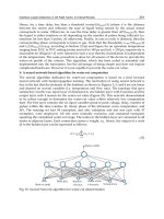
Fig. 2. (a) RF output power vs. optical input power. (b)Optical spectrum and RF spectra : (c)
around 10.5 GHz, (d) around 5.25 GHz
in half by the frequency divider. The signal is amplified with the RF amplifier and positively
fed back to the electrode of the modulator. If a lightwave with enough intensity is launched
into the modulator, the loop gain of the oscillator becomes greater than one, and then the OEO
starts oscillating. In this OEO, the oscillation frequency, f
0
, is half the frequency of the optical
beat between the USB and LSB components generated by the modulator. At the output of the
photodetector, the photocurrent contains 2f
0
frequency components, while the frequency of
the driving signal at the MZM is f
0
.
We explain here why the use of a frequency divider is essential in the
π
2
-shift bias operation.
When the MZM is driven with a sinusoidal signal at repetition frequency f
0
,theopticalfield
of the EO-modulated lightwave is given as
E
out

=
1
2
E
in
∞
∑
k=∞

J
k
(A
1
)e
jkωt+θ
2
+ J
k
(A
2
)e
jkωt+θ
2

,
where E
in
is the input field, and J
k
(·) denotes the k-th order Bessel functions. The photocurrent

of the direct-detected signal can be written as
i
ph
=
η|E
in
|
2
2

1
+ cos Δθ

J
0
(ΔA)+2
∞
∑
k=1
(−1)
k
J
2k
(ΔA) cos 2kωt

−sinΔθ

2
∞
∑

k=1
(−1)
k
J
2k−1
(ΔA) cos(2k −1)ωt

,
where η is the conversion efficiency of the photodiode. The amplitude of each mode at kf
0
is a sinusoidal function of bias V. It should be noted that the odd-order harmonic modes of
the detected photo current are governed by sine functions, whereas the even-order modes are
governed by cosine functions. In conventional OEOs, the fundamental mode at f
0
is fed back
to the modulation electrode, where i
ph
is maximized at the quadrature bias point (Δθ = ±
π
2
)
but minimized at the zero/top-biased conditions. Therefore, less feedback gain is obtained
in an OEO if the MZM is biased around the zero or top point. In the proposed OEO, on the
other hand, the frequency divider divides the frequency in half so that the second-order mode
is fed back to the modulation electrode. In this case, the feedback gain is minimized at the
quadrature bias condition, Δθ
=
π
2
, and maximized at the zero/top bias conditions, Δθ =

0, ±π. An optical two-tone signal is generated by using the OEO employing an push-pull
operated MZM biased at the null point.
319
Optoelectronic Circuits for Control of Lightwaves and Microwaves
8 Name of the Book
λ
Δλ
filter window
PM signal
λ
0
Photodiode
Amplifier
Laser diode
Harmonic
modulator
f0
N f0
f0
Optical
Electrical
Optical frequency comb
output
(a) (b)
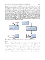
Fig. 3. (a) Concept of the OEO made of a harmonic modulator for optical frequency comb
generation. (b) Offset filtering to convert phase-modulated lightwave to intensity-modulated
feed-back signal.
Figure 2(a) shows threshold characteristics of the OEO, where RF output power is plotted
against optical input power. Increasing the optical input power to the OEO, it started
oscillating and the oscillation was stably maintained. The input power at the threshold

for oscillation was 0.1 mW. The trace of the oscillation characteristics of the OEO is largely
different from that of a conventional OEO. In our OEO output RF power is proportional
to the square of the optical imput power, whereas conventional OEOs have square-root
input-to-output transfer function. This is because the RF signal introduced back to the
modulation electrode is clipped to a constant level by the frequency divider comprised of a
logical counter. The optical input power does not change the feedback signal level; therefore,
the output RF power is proportional to the square of the input power.
The optical output spectrum is shown in Fig. 2(b). An optical two-tone signal was successfully
generated. The RF spectra before and frequency division are also shown in the inset of
Fig. 2 (c)(d). The upper trace (c) indicates the spectrum of the signal at the input of the
frequency divider. A 10.5-GHz single-tone spectrum was obtained there. The RF spectrum of
the frequency-divided signal, which drives the modulator, is shown in the lower trace (d). In
both spectra, side-mode suppression ratios were more than 50 dB, which can be improved by
using a more appropriate BPF with a narrower frequency passband.
In this subsection, an optoelectronic oscillator employing a Mach-Zehnder modulator biased
at the null/top conditions has been described, which is suitable for generating optical
two-tone signals. Under the bias conditions, a frequency divider implemented in the OEO
was crucial for extracting a feedback signal from the upper- and lower-sideband components
of an electro-optic modulated lightwave.
3.3 Comb generation
Optical frequency comb generators can provide many attractive applications in micro-wave or
millimeter-wave photonic technologiesJemison (2001): such as, optical frequency standard for
absolute frequency measurement systems, local-oscillator remoting in radio-on-fiber systems,
control of phased array antenna in radio astronomy systems, and so on.
Conventionally, a mode-locked laser is a popular candidate for such an optical frequency
comb generation Arahira et al. (1994). Viewed from a practical perspective, however, the
technology has difficulties in control of starting and keeping the state of mode-locking. This
is because typical mode-locked lasers, consisting of multi-mode optical cavities, have multi
stabilities in their operations. In this subsection, an OEO modified for comb generation
is described: optoelectronic oscillator (OEO) made of a harmonic modulator is described.

Sakamoto et al. (2006b)Sakamoto et al. (2007b)Sakamoto et al. (2006a)
320
Optoelectronics - Materials and Techniques
Optoelectronic Circuits for Control of
Lightwaves and Microwaves 9
0.8π 1.2π
(a) (b)
Fig. 4. (a) Optical intensity of each harmonic components against optical input power.
Squares: at the carrier, dots: at the 1st-order, triangles: 2nd-order, circles: 3rd-order
components. (b) Optical spectrum generated from the OEO (wavelength resolution = 0.01
nm).
It is known that EO modulation with larger amplitude signal promotes generating
higher-order harmonics of the driving signal, obeying Bessel functions as discussed in the
next section in detail. The OEO described in this subsection aims at the generation of
frequency components higher than the oscillation frequency. In the OEO, an optical phase
modulator is implemented in its oscillator cavity and driven by large-amplitude single-tone
feed-back signal. Even this simple setup can generate multi-frequency components, i.e.
optical frequency comb, with self oscillation as well as the conventional mode-locked lasers
do. The most important difference from the mode-locking technologies is that the proposed
comb generator is intrinsically a single-mode oscillator at a microwave frequency. Therefore,
it is much more easy to start and maintain the oscillation comparing to the mode locking.
A regenerative mode-locked laser is one of the successful examples of the wideband signal
generation based on OEO structure, where a laser cavity is constructed in the optical
part. However, it still relies on complex laser structure, whilw haronic-OEO has a single
one-direction optical path structre without laser caivity.
Figure 3(a) shows the schematic diagram of the proposed OEO. The OEO consists of an
optical harmonic modulator, a photodetector, and an RF amplifier. The harmonic modulator
generates optical harmonic components of a modulation signal. The photodetector, connected
at the output of the modulator, converts the fundamental modulation component ( f
0

)into
an RF signal. The signal is amplified with the RF amplifier and led to the electrode of the
modulator. If a lightwave with enough intensity is launched on the input of the harmonic
modulator, the OEO starts oscillation because the fundamental modulation component at the
frequency of f
0
is positively fed back to the modulator. Note that harmonic components (Nf
0
)
are generated at the output of the harmonic modulator, while the OEO is oscillating at f
0
.
Contrast to the conventional mode-locked lasers, the generated harmonics does not contribute
to the oscillation, so that the OEO yields much more stable operation without complex control
circuitry.
In this paper, an optical phase modulator is applied to the harmonic modulation in the
OEO, where the modulator is driven by an RF signal with large amplitude. The modulator
easily generates higher-order frequency components over the bandwidth of its modulation
electrode. In order to achieve optoelectronic oscillation, it is required to detect feed back
signal from the phase-modulated (PM) lightwave. For this purpose, we apply optical
asymmetric filtering on the PM components, as shown in Fig. 3(b). By giving some
frequency offset between the lightwave and the optical filter, the PM signal is converted into
321
Optoelectronic Circuits for Control of Lightwaves and Microwaves
10 Name of the Book
intensity-modulated (IM) signal. This scheme is effective especially when the bandwidth of
the filter is narrower than that of the PM signal. A fiber Bragg grating (FBG) is suitable for
such an asymmetric filtering on deeply phase modulated signal since its stop band is typically
narrower than the target bandwidth of frequency comb to be generated ( 100 GHz).
The OEO was made of an LiNbO

3
optical phase modulator, an optical coupler, an FBG, a
photodiode (PD), an RF amplifier, a band-pass filter (BPF) and an RF delay line. The FBG
had a 0.2-nm stop band and its Bragg wavelength was 1550.2 nm. The BPF determined the
oscillation frequency of the OEO, and its center frequency and bandwidth of the BPF were
9.95 GHz and 10 MHz, respectively. The delay line aligned the loop length of the OEO to
control the oscillation frequency, precisely. A CW light launched on the OEO was generated
from a tunable laser diode (TLD). The center wavelength was aligned at 1550 nm, which was
just near by the FBG stop band. The output lightwave from the FBG was photo-detected with
the PD and introduced into the electrode of the phase modulator followed by the BPF and the
amplifier. The harmonic modulated signal was tapped off with the optical coupler connected
at the output of the modulator.
Increasing the optical power launched on the phase modulator, the OEO started oscillating.
Fig. 4(a) shows optical output power of the phase-modulated components as a function of
input power of the launched CW light. The squares, dots, triangles and circles indicate the
0th, 1st, 2nd and 3rd-order harmonic modulation components, respectively. As shown in
Fig. 4(a), the input power at the threshold for oscillation was around 50 μW. Then, at the
optical input power of 140 μW, we measured the optical spectrum of the generated signal.
The output spectrum of the generated frequency obtained at (C) is shown in Fig.4 (b). Optical
frequency comb with 120-GHz bandwidth and 9.95-GHz frequency spacing was successfully
generated. The single-tone spectrum indicates that the OEO single-mode oscillated at the
frequency of 9.95 GHz. The frequency spacing of the generated optical frequency comb was
accurately controlled with a resolution of 30 kHz. By controlling the delay in the oscillator
cavity, the oscillation frequency was continuously tuned within the passband of the BPF; the
tuning range was about 10 MHz. The maximum phase-shift available in our experimental
setup was restricted to about 1.7π [rad]. It is expected that more deep modulation using
a high-power RF amplifier and/or a low-driving-voltage modulator would generate more
wideband frequency comb.
In conclusion, in this subsection, an optoelectronic oscillator made of a LiNbO
3

phase
modulator for self-oscillating frequency comb generation has been described. Deeply
phase-modulated light was converted to intensity-modulated signal through asymmetric
filtering by an FBG, and fed back to the modulator. Frequency comb generation with 120-GHz
bandwidth and 9.95-GHz accurate frequency spacing was achieved. The frequency spacing of
the comb signal was tunable in the range of 10 MHz with the resolution higher than 30 kHz.
The comb generator was selfstarting single-mode oscillator and stable operation was easily
achieved without complex control technique required for conventional mode-locked lasers.
4. Spectral enhancement and short pulse generation by photonic harmonic mixer
Generation of broadband comb and ultra short pulse train have been investigated for long
time Margalit et al. (1998); Yokoyama et al. (2000); Yoshida & Nakazawa (1998); ?); ?); ?); ?);
?); ?. Especially in the last decade, compact and practical comb/pulse sources have been
rapidly improved in the areas of test and measurements, optical telecommunications, and so
on, accelerated by progress in semiconductor and fiber optics. For test and measurements,
optical fiber mode-locked lasers based on passive mode-locking have been developed into
compact packages, which can simply generate pulse train in femto-second region with a high
322
Optoelectronics - Materials and Techniques
Optoelectronic Circuits for Control of
Lightwaves and Microwaves 11
peak power of k - MWatt and a repetition rate of MHz or so Arahira et al. (1994). The
technology is also useful for generation of ultra broadband optical comb that covers octave
bandwidth. For telecomm use, active mode locked lasers and regenerative mode-locked lasers
based on semiconductor or fiber laser structures have been intensively investigated, so far
???. Optical combs generated from the sources have large frequency spacing and they can
be utilized as multi-wavelength carriers for huge capacity transmission. They are also useful
for ultra high-speed communications because the pulse train generated is in high repetition.
For practical use, however, stabilization technique is inevitable for keeping mode-locked
lasing operation. Flexible controllability and synchronization with external sources are also
important issues.

Recently, approaches based on electro-optic (EO) synthesizing techniques are becoming
increasingly attractive Kourogi et al. (1994). Behind this new trend, we know rapid
progress in EO modulators like LiNbO
3
- and semiconductor-based waveguide modulators
with improved modulation bandwidth and decreased driving voltage Kondo et al. (2005);
Sugiyama et al. (2002); Tsuzuki et al. (n.d.). In the approaches, wideband optical comb with
a bandwith of several 100 GHz-THz and picosecond (or less) pulse train at a repetition of
10 100 GHz are generated from continuous-wave (CW) sources, which do not rely on any
complex laser oscillation or cavity structures. This is of a great advantage for stable and
flexible generation of optical comb/pulses.
In the former section, we described self-oscillating comb generation based on OEO
configuration, where it is clarified that comb generation can be achieved without loosing
features of single-mode oscillators. The modulator used in the harmonic OEO is phase
modulator in that case. As discussed in the section, EO modulators are useful way for the
comb generation because it is superior in stable and low-phase-noise operation. A difficulty
remained is to flatly generate optical comb; in other words, it is difficult to generate optical
comb which has frequency components with the equal intensity. In fact, with a use of a phase
modulator the amplitude of each frequency component obeys Bessel’s function in different
order, thus we can see that the spectral profile is far from flat one. Looking at applications
of the comb sources, it can be clearly understood why lack or weakness of any frequency
components causes problems. If we consider to use the comb source in WDM systems, for
example, each channel should has almost equivalent intensity; otherwise the channels with
weak intensity has poor signal-to-ratio characteristics; the high-intensity channel suffers from
nonlinear distortion through transmission. One of the possible ways to solve this problem is
to apply an optical filter to the non-flat comb. However, this approach has some problems. To
equalize and make the comb signal flat, the filter should have special transmittance profile.
In addition, the efficiency of the comb generation would be worse because all components
would be equalized to the intensity level of the weakest one.
In this section, we focus on this issue: flat comb generation by using electro-optic modulator,

where a flat comb is generated by a combination of two phase-modulated non-flat comb
signals. By this method, spectral ripples between the two phase-modulated lights are
cancelled each other to form a flat spectral profile. An noticeable point of this method is
that only single interferometric modulator is required for the operation. Another point is that
the flat comb is generated from CW light and microwave sources, and no optical cavities are
required.
First, in this section, flat comb generation and its theory is described. Four principle
modes of operation are clarified, which are essential for the flat comb generation by two
phase-modulated lights. Next, synthesis of optical pulse train from the flat comb is described.
Spectral enhancement and/or pulse compression with an aid of nonlinear fiber is also
discussed.
323
Optoelectronic Circuits for Control of Lightwaves and Microwaves
12 Name of the Book
BiasRF-b
RF-a
A1 sin ωt
A
2 sin ωt
Δθ
−Δθ
Bias
Ein Eout
λ λ
ω
λ0 λ0
λ
λ
Fig. 5. Concept of ultraflat optical frequency comb generation using a conventional
Mach-Zehnder modulator. A CW lightwave is EO modulated by a dual-drive Mach-Zehnder

modulator driven with large sinusoidal signals with different amplitudes.
4.1 Ultra-flat comb generation
Fig. 5 shows the principle of flat comb generation by the combination of two phase modulated
lightwaves Sakamoto et al. (2007a). In the optical frequency comb generator, an input
continuous-wave (CW) lightwave is EO modulated with a large amplitude RF signal using
a conventional MZM. Higher-order sideband frequency components (with respect to the
input CW light) are generated. These components can be used as a frequency comb because
the signal has a spectrum with a constant frequency spacing. Conventionally, however, the
intensity of each component is highly dependent on the harmonic order. We will find, in this
section, that the spectral unflatness can be cancelled if the dual arms of the MZM are driven
by in-phase sinusoidal signals, RF-a and RF-b in Fig. 5, with a specific amplitude difference.
4.1.1 Principle opetation modes for flat comb generation
Here, in this subsection, principle operation modes for flatly generating optical comb using
an MZM are analytically derived. Sakamoto et al. (2007a)
Suppose that the optical phase shift induced by signals RF-a and RF-b are Φ
a
(t)=(A +
ΔA) sin
(
2π f
0
t + Δφ
ab
)
, Φ
b
(t)=(A − Δ A) sin
(
2π f
0

t −Δφ
ab
)
, respectively, where A is the
average amplitude of the zero-to-peak phase shift induced by RF-a and Rf-b; 2ΔA is difference
between them; f
0
is the modulation frequency; 2Δφ
ab
is the phase difference between RF-a and
RF-b.
For large-amplitude driving signals, power conversion efficiency from the input CW light to
each harmonic mode can be asymptotically approximated as
η
k
≡
P
k
P
in
≈
1
2πA



e
æ(Δθ+kΔφ
ab
)

cos(α + ΔA)+e
−æ(Δθ+kΔφ
ab
)
cos(α −ΔA)



2
=
1
2πA
[
1 + cos(2ΔA) cos(2Δθ + 2kΔφ
ab
)+cos(2ΔA) cos β cos(kπ)
+
cos
(
2Δθ + 2kΔφ
ab
)
cos β cos
(
kπ
)]
(1)
,whereβ
≡ A −
π

2
(+Higher −order term). This expression describes behavior of the
generated comb well as long as
A is large enough. Generally, the conversion efficiency
is highly dependent on the harmonic order of the driving signal, k, which means that the
frequency comb generated from the MZM has a non-flat spectrum.
324
Optoelectronics - Materials and Techniques
Optoelectronic Circuits for Control of
Lightwaves and Microwaves 13
LD
Bias
Optical spectrum
analyzer
RF-b
RF-a
λ=1550 nm
P=5.8 dBm
PC
φ
10 GHz
ATT
MZM
RF spectrum
analyzer
Autocorrelator
PD
EDFA
SMF
(500 m~1500 m)

(a) Ultra-flat comb Generation
(b) Pulse synthesis
BPF
w/o
or w/ 3 nm
or w/ 1 nm
1100 m
Fig. 6. Experimental setup; LD: laser diode, PC: polarization controller, MZM: Mach-Zehnder
modulator, ATT: RF attenuator, EDFA: Erbium-doped fiber amplifier, BPF: optical bandpass
filter, SMF: standard single-mode fiber, PD: photodiode.
To make the comb flat in the optical frequency domain, the intensity of each mode should be
independent of k. From Eq. 1, the condition is
cos
(2ΔA)+cos
(
2Δθ + 2kΔφ
ab
)
=
0(2)
To keep this equation for any k, the second term should be independent of k. Δφ
ab
should
satisfy
Δφ
ab
= 0or ±
π
2
.(3)

It should be noted that Δφ
ab
= 0andΔφ
ab
=
π
2
correspond to the cases of “in-phase” and
“out-of-phase (push-pull)” driven conditions, respectively.
In the “in-phase” driven case (Δφ
ab
= 0), the difference of the induced phase difference and
bias difference should be related as
ΔA
±Δθ = nπ +
π
2
.(4)
to make the spectral envelope flattened. Sakamoto et al. (2007a)
In the case of Δφ
ab
=
π
2
, the MZM is allowed to be “out-of-phase (push-pull)” driven
Sakamoto et al. (2011). From Eq. 2, the flat spectrum condition yields
ΔA
= ±
π
4

, Δθ
= ±
π
4
(5)
From Eq. 4 and Eq. 5, it is found that there are conditions for flat frequency comb generation
both for “in-phase” and “out-of-phase” driving cases, and the former condition is more robust
since we only need to keep the balance between ΔA and Δθ. If we make the efficiency of the
generated comb maximum, however, the driving condition for “in-phase” driven case also
results in ΔA = ±
π
4
, Δθ = ±
π
4
.
4.1.2 Experimental proof
Next, the flat spectrum condition in the four operation modes are experimentally proved. Fig.
6 shows the experimental setup, which is commonly referred in this chapter hereafter. The
optical frequencycomb generator consisted ofa semiconductor laser diode(LD) and a LiNbO
3
dual-drive MZM having half-wave voltage of 5.4 V. A CW light was generated from the LD,
whose center wavelength and intensity of the LD was 1550 nm and 5.8 dBm, respectively. The
325
Optoelectronic Circuits for Control of Lightwaves and Microwaves
14 Name of the Book
0
5
10
15

20
0 50 100 150 200 250 300
Intensity, mW
Time, ps
0
5
10
15
20
0 50 100 150 200 250 300
Intensity, mW
Time, ps
Fig. 7. Optical spectra; (a) Single-arm driven, (b) Δ
p
hi = 0 (in-phase), (c) Δ
p
hi = 0.4π,(d)
Δ
p
hi = 0 (out-of-phase), Optical waveforms measured with an four-wave-mixing-based
all-optical sampler (temporal resolution = 2 ps); (a) in-phase mode, (b) out-of-phase mode
CW light was introduced into the modulator through a polarization controller to maximize
modulation efficiency. The MZM was dual-driven with sinusoidal signals with different
amplitudes (RF-a, RF-b). The RF sinusoidal signal at a frequency of 10 GHz was generated
from a synthesizer, divided in half with a hybrid coupler, amplified with microwave boosters,
and then fed to each modulation electrode of the modulator. The intensity of RF-a injected
into the electrode was attenuated a little by giving loss to the feeder line connected with the
electrode. The input intensities of RF-a and RF-b were 35.9 dBm and 36.4 dBm, respectively
Sakamoto et al. (2008). In order to select the operation modes, mechanically tunable delay
line with tuning range over 100 ps was implemented in the feeder line for RF-a. The

modulation spectra obtained from the frequency comb generator were measured with an
optical spectrum analyzer. Optical waveform was measured with a four-wave-mixing-based
all-optical sampler having temporal resolution of 2 ps.
Fig. 7 shows the optical spectra of the generated frequency comb. (a) is the case obtained
when the MZM was driven in a single arm, where the driving condition was far from the
“flat-spectrum” condition. (b) is the spectrum under the “flat-spectrum” condition in the
“in-phase” operation mode. The delay between the RF-a and RF-b was set at 0 (Δφ
ab
= 0).
The RF power of the driving signals were 35.9 dBm and 36.4 dBm, respectively. Keeping the
intensities of the driving signals, delay between RF-a and RF-b was detuned from Δφ
ab
= 0.
The spectral profile became asymmetric as shown in (c), where Δφ
ab
≈ 0.2π.Thespectrum
became flat again when Δφ
ab
=
π
2
as shown in (d). The spectral at (b) and (d) were almost the
same as expected and the 10-dB bandwidth was about 210 GHz in the experiments. Optical
spectra with almost same the profile was monitored even when the optical bias condition was
changed from the up-slope bias condition to the down-slope one. It has been confirmed that
there are totally four different operation modes for flat comb generation using the MZM.
Characterization of the temporal waveform helps account for the behavior of the operation
modes. Fig. 7 shows the optical waveforms measured with the all-optical sampler. Fig. 7(a) is
the case obtained when the MZM was operated in the in-phase mode. The optical waveform
was sinusoidal like since the optical amplitude is modulated within the range between 0 to

π under the condition. On the other hand, Fig. 7(b) is measured at the push-pull operation
mode. In this case, the temporal waveform was sharply folded back and forth and it is found
that the optical amplitude was over swang far beyond the full-swing range of 0-π.
326
Optoelectronics - Materials and Techniques
Optoelectronic Circuits for Control of
Lightwaves and Microwaves 15
1
10
100
0 10 20 30
Normalized bandwidth
Induced phase shift, rad
0.001
0.01
0.1
1
0 10 20 30
Conversion efficiency
Induced phase shift, rad
(a) (b)
Δω/ω > 10
Δω/ω > 10
Fig. 8. (a) Maximum conversion efficiency, η
k,max
vs. induced phase shift A; theoretically
(asymptotically) [solid line] and numerically averaged conversion efficiency within 0.5Δω
[squares];(b) bandwidth, Δω,vs.
A; theoretically (asymptotically) (Δω)[solid line], number of
CW components within 3-dB drop of η

k
[squares], fitted curve (0.67Δω) [dashed line]; in each
graph, the region of Δω/ω
> 10 is practically meaningful, where more than 10 frequency
components are generated.
4.1.3 Characteristics of optical frequency comb generated from single-stage MZM
Here, primary characteristics of the generated comb are described providing with additional
analysis. Conversion efficiency, bandwidth, noise characteristics are analyzed, in this
subsection.
Conversion Efficiency
The output power should be maximized for higher efficient comb generation. Here, we
discuss efficiency of comb generation. First, we define two parameters that stands for
conversion efficiency of the comb geenration. One is a “total conversion efficiency”, which is
defined as the total output power from the modulator to the intensity of input CW light. The
other is simply called “conversion effciency”, which is defined as the intensity of individual
frequency component to the input power.
Under the flat spectrum condition for “in-phase” mode, Eq. 3, the intrinsic conversion
efficiency, excluding insertion loss due to impairment of the modulator and other extrincic
loss, is theoretically derived from Eq. 1 and Eq. 4, resulting in
η
k
=
1 −cos4Δθ
4πA
,(6)
which means that the conversion efficiency is maximized upto
η
k,max
=
1

2πA
,whenΔA
= Δθ =
π
4
.(7)
Note that this is the optimal driving condition for flatly generating an optical frequency
comb with the maximum conversion efficiency. Hereafter, we call this equation the
“maximum-efficiency condition” for ultraflat comb generation.
For the out-of-phase operation mode, the conversion efficiency yields,
327
Optoelectronic Circuits for Control of Lightwaves and Microwaves
16 Name of the Book
η
k,out−of−phase
=
1
2πA
,(8)
, which is equivalent with the maximum-efficiency condition for the inphase operation mode,
Eq. 7.
Fig. 8(a) shows the maximum conversion efficiency, η
k,max
plotted against the average
induced phase shift of
A. The solid curve indicates the theoretically derived conversion
efficiency, Eq. 7 or 8. The squares in the plot indicate the numerically calculated
average conversion efficiencies within the 0.5Δω bandwidth with respect to each value of
A. For the calculation, optical spectrum of the generated comb is calculated by using
a First-Fourier-Transform (FFT) method, which is commonly used for spectral analysis of

modulated lightwave. The range of
A for the calculation is restricted in the rage of
Δω
ω
> 10,
where the generated comb has practically sufficient number of frequency components. The
good agreement with numerical data proves that Eq. 7 or 8 is valid in the practical range.
Bandwidth
Bandwidth of the comb under the flat spectrum conditions is estimated, here. Under the
flat spectrum conditions, energy is equally distributed to each frequency component of the
generated comb. From the physical point of view, however, the finite number of the generated
frequency comb is, obviously, allowed to have the same intensity in the spectrum; otherwise,
total energy is diverged. The approximation for Eq. 1 is valid as long as k
<< k
0
and η
k
rapidly approaches zero for k >> k
0
. It is reasonable to assume that optical energy is equally
distributed to each frequency mode around the center wavelength (i.e. k
<< k
0
). Since the
total energy,
P
out
, can be calculated in time domain, the bandwidth of the frequency comb
becomes
Δω

=
P
out
ω
η
k
P
in
≈ πAω (for small ΔA),(9)
which is almost independent of ΔA (or Δθ).
As for the comb generated under the out-of-phase operation mode, the analysis also results in
the same bandwidth.
In Fig.8(b), the bandwidth, Δω is plotted as a function of
A. In the graph, the solid curve
indicates the theoretical bandwidth derived in Eq. 9; the squares represent the calculated 3-dB
bandwidths required for keeping conversion efficiency of less than 3-dB rolling off from the
center wavelength. These data almost lie on the fitted curve of 0.67Δω, which is also plotted
as a dashed curve in the graph. From this analysis, frequency components within 67% of the
theoretical bandwidth of Δω are numerically proven to have sufficient intensity with less than
a 3-dB drop in the conversion efficiency. The 33% difference from the predicted Δω is mainly
because the shape of actual spectrum of the generated comb slightly differs from a rectangle
assumed in the derivation of Eq. 7.
4.2 Linear pulse synthesis
Generation of picosecond optical pulse train at a high repetition rate ?????? has been
extensively studied to achieve highly stable and flexible operation, aiming at the use
in ultra-high-speed data transmission or in ultra-fast photonic measurement systems.
Conventionally, actively/passively mode-locked lasers based on semiconductor or fiber-optic
328
Optoelectronics - Materials and Techniques
Optoelectronic Circuits for Control of

Lightwaves and Microwaves 17
BiasRF-b
RF-a
A1 sin ωt
A
2 sin ωt
Δθ
−Δθ
Bias
Spectral shaping
CW light
Parabolic phase
compensation
MZM
Pulse outpu
t
Dispersive fiber
D
Bandpass
filter
(a) Ultra-flat comb generation (b) Pulse synthesis
Fig. 9. Generation of ultra-short pulses by using a single-stage conventional Mach-Zehnder
modulator.
technologies have been typically used to generate such pulse trains ???. In the technologies,
however, the laser cavity should be strictly designed and stabilized to generate stable pulse
trains, which reduces flexibility in the operation. Especially, its repetition rate of the generated
pulses is almost fixed and its scarce tunability has been provided. In addition, the highly
nonlinear properties involved in generating pulses also restrict its operating conditions, which
leads to limited output optical power and to uncontrollable chirp characteristics.
In the previous section, ultra-flat frequency comb generation by using only an MZM has

been described. In this section, we apply it to generation of ultrafast pulse train. Basically,
the strategy to synthesize optical pulse train from the comb source is as follows: (1) Phase
differences between frequency components are aligned to be zero to form impulsive pulse
train. (2) Profile of temporal waveform is controlled by spectral shaping to the generated
comb.
By this approach, pulse trains with a pulse width of picosecond order can be obtained as
discussed in this section. These two operations can be achieved in a linear process by simple
passive components, as discussed in this section. The first one, phase comensation, is easily
achieved by using acommonly usedoptical dispersive fiber. The second one, spectral shaping,
is also achieved with a typical optical bandpass filter. Thin-film filters can be used for this
puropose.
Figure 9 shows the basic construction of the picosecond pulse generator employing
single-stage MZM. The pulse source consists of two sections: one for (a) comb generation
and the other for (b) pulse synthesis. Section (a), consisting of a single-stage MZM, has a
role to flatly generate a frequency comb. In this section, a continuous-wave (CW) light is
EO modulated with the MZM, which is dual-driven by sinusoidal in-phase or out-of-phase
signals having different amplitudes. Section (b), on the other hand, is comprised of an optical
filter and a fiber, and it spectrally shapes the generated comb into a pulse train having a
sync
2
-like or a Gaussian-like temporal waveform.
The advantages of this pulse source are 1) the pulses are generated in an optically linear
process, so that the optical level of the generated pulse is easily controlled; 2) the pulse
source can be started up quickly without the need for complicated control procedures; 3) the
repetition rate and the center wavelength of the generated pulse can be flexibly and quickly
controlled; 4) the generated pulse train is highly stable due to the simple structure of the pulse
generator and to the maturity of the components employed; 5) the pulse generator guarantees
ultra-low timing jitter due to the high coherence of the generated comb.
Phase characteristics of comb
To clarify the phase characteristics of the generated comb, we modify Eq. 1 to look into

higher-order terms of the output field, yielding
329
Optoelectronic Circuits for Control of Lightwaves and Microwaves
18 Name of the Book
E
out
=
1
2
E
in
∞
∑
k=−∞

J
k
(A
1
)e
j(kωt+θ
1
)
+ J
k
(A
2
)e
j(kωt+θ
2

)

≈
E
0
2

2
π
A
−
1
2
∞
∑
k=−∞

cos

A −
(
2k + 1)π
4
+
4k
2
−1
2
8
A

−1
+ ΔA

e
æΔθ
cos

A −
(
2k + 1)π
4
+
4k
2
−1
2
8
A
−1
−ΔA

e
−æΔθ

e
æ(θ+kωt)
, (10)
Since we have already derived the flat spectrum conditions, we substitute Eq. 3 and Eq. 4 into
Eq. 10, respectively. Under the flat spectrum condition for in-phase and out-of-phase modes,
respectively, the amplitude and the phase of the frequency modes can be approximated as

A
k
=
E
0
sin(2Δθ)
√
2πA
, Φ
k
= ±
4k
2
−1
8A
, (11)
where those series higher than the fourth order series of Φ
k
are neglected. It should be
noted that the amplitude is independent of the harmonic order of the generated frequency
components, k; the optical phases of the modes are related through a parabolic function of k.
This equation is valid as long as
|k| << k
max
= πA is satisfied.
Linear pulse synthesis by fiber-optic circuits
0
5
10
15

20
0 200 400 600 800 1000 1200 1400 1600
Pulse width, ps
SMF length, m
Fig. 10. Pulse width measured as a function of SMF length; solids: w/o filter, squares: w/
3-nm filter, triangles: w/ 1-nm filter
Next, it is explained how the generated ultra-flat frequency comb is shaped into an ultra-short
pulse train in section (b) of the pulse source by using Fourier spectral synthesis. In the case
of in-phase operation mode, the story becomes more simple. From Eq. 11, it is found that the
optical phase relationship between each mode is in a parabolic function of the mode number.
Note that phase compensation with
−Φ
k
makes the temporal waveform of the generated
comb impulsive. Such a phase compensation can be easily achieved by using a piece of
standard optical fiber that gives a parabolic phase shift, i.e., a counter group delay, to the
generated comb. The optimal length for the pulse generation is simply obtained as,
L
= ∓
∂
2
Φ
k
∂k
2
(β
2
ω
2
0

)
−1
= ∓(β
2
Aω
2
0
)
−1
, (12)
where β
2
denotes group velocity dispersion in the fiber.
330
Optoelectronics - Materials and Techniques
Optoelectronic Circuits for Control of
Lightwaves and Microwaves 19
-0.2
0
0.2
0.4
0.6
0.8
1
-20 -10 0 10 20
Autocorrelation, a.u.
Delay, ps
-0.2
0
0.2

0.4
0.6
0.8
1
-20 -10 0 10 20
Autocorrelation, a.u.
Delay, ps
-0.2
0
0.2
0.4
0.6
0.8
1
-20 -10 0 10 20
Autocorrelation, a.u.
Delay, ps
-50
-40
-30
-20
-10
0
1548.5 1549 1549.5 1550 1550.5 1551
Intensity, dBm
Wavelength, nm
-50
-40
-30
-20

-10
0
1548.5 1549 1549.5 1550 1550.5 1551
Intensity, dBm
Wavelength, nm
-50
-40
-30
-20
-10
0
1548.5 1549 1549.5 1550 1550.5 1551
Intensity, dBm
Wavelength, nm
(a)
(b)
(c)
Δt (Gaussian)
=2.4 ps
Δt (Gaussian)
=3.0 ps
Δt (Gaussian)
=3.9 ps
Fig. 11. Optical spectra (left side) and autocorrelation traces (right side); (a) W/o filtering, (b)
sync
2
-like shape, (c) Gaussian-like shape.
The synthesized pulse train, however, has a rather temporal waveform of the sync
2
function

causing a large pedestal around the main pulse, because the generated comb has a rectangular
spectrum. In many cases, it is required to shape the temporal waveform of the pulse into
Gaussian to suppress the undesired pedestal. If an optical bandpass filter (OBPF) is applied
to the generated comb having a cut-off frequency of f
<<
1
2π
k
max
ω, the spectral envelope
is shaped into the passband profile of the OBPF; thus, the temporal waveform should be a
Fourier transform of the filter passband profile. For instance, if a Gaussian filter is applied to
the generated comb together with the appropriate phase compensation of
−Φ
k
,itispossible
to generate Fourier-transform limited Gaussian pulse train with a pulse width of T
= 0.44/ f
and with a repetition of T
0
=
2π
ω
. From this analysis, it is found that the optical pulses can be
generated only using linear fiber-optic components. This has numerous practical advantages.
Experimental proof
Figure 6 shows the experimental setup for picosecond pulse generation using a single-stage
MZM. In section (a) of the setup, an ultra-flat frequency comb was generated. A CW light was
generated from a laser diode (LD), whose center wavelength and intensity were 1550 nm and
5.8 dBm, respectively. The CW light was introduced into the conventional LiNbO

3
dual-drive
MZM that was driven under the flat spectrum condition. The MZM, having half-wave voltage
of 5.4 V, was dual-driven with 10-GHz sinusoidal signals of RF-a and RF-b. The RF signals
were generated from a synthesizer, divided in half with a hybrid coupler, amplified with
microwave boosters, and fed into the electrodes of the modulator. The intensity of the RF-a fed
into the electrode was attenuated a little by giving loss to the feeder line connected with the
electrode. The average input intensity of RF-a and of RF-b was 38.5 dBm, and the difference
between them was 1.0 dB. The average zero-to-peak deviation in the phase shift induced in
the modulator was estimated to be 4.3 π. The phase difference between RF-a and RF-b was
aligned to be zero by using a mechanically tunable delay line placed in the feeder cable for
RF-a.
331
Optoelectronic Circuits for Control of Lightwaves and Microwaves
20 Name of the Book
-25
-20
-15
-10
-5
0
5
10
1500 1520 1540 1560 1580 1600
Intensity, dBm
Wavelength, nm
-0.2
0
0.2
0.4

0.6
0.8
1
-15 -10 -5 0 5 10 15
Autocorrelation, a.u.
Delay, ps
Fig. 12. Characteristics of generated pulse train; (a) optical spectrum , (b) autocorrelation
traces, dotted: seed pulse, solid: compressed pulse
In section (b) of the experimental setup, the generated comb was converted into a pulse
train. The comb was amplified with an Erbium-doped fiber amplifier (EDFA), and led to
an optical thin-film band-pass filter (OBPF) followed by a piece of standard single-mode fiber
(SMF). In addition to the function of the spectral shaping, the OBPF filtered out ASE noise
generated from the EDFA. The characteristics of the generated pulse train were evaluated
with an optical spectrum analyzer and an autocorrelator, and the timing jitter was analyzed
with an RF spectrum analyzer.
First, in this experiment, the length of the SMF was optimized by evaluating evolution of the
pulses through the fiber. Figure 10 shows pulse width dependence measured as a function
of the SMF length. The pulse width was estimated from the autocorrelation traces assuming
the Gaussian waveform. The circles, squares and triangles in the graph correspond to pulse
widths measured (a) without a filter, (b) with a 3-nm filter (Δλ
bpf
= 3 nm) and (c) with a 1-nm
filter (Δλ
bpf
= 1 nm). We found that
˜
1100 m is the optimal length for the pulse synthesis,
where a group delay of 22 ps
2
/nm was introduced. Thus, the experimentally optimized

length of the SMF is in good agreement with the theoretical value estimated from Eq. 12.
Figure 11 shows the optical spectra and the autocorrelation traces of the generated pulse
trains. The narrowest pulse was obtained without using the OBPF, where the pulse width was
estimated to be 2.4 ps. In this case, however, the pulse train had a large pedestal around the
mainlobe of the pulse. For Δλ
bpf
= 3 nm, the temporal waveform was a sync
2
-like function
since the shape of the spectral envelope was square. The estimated pulse width was 3.0-ps.
In the case of Δλ
bpf
= 1 nm, which is narrower than the spectral width of the generated
comb, the optical spectrum had almost the same shape as the passband of the OBPF. It is
confirmed that a Gaussian-like pulse train with a pulse width of 3.9 ps was generated, where
time-bandwidth product was 0.45. The root-mean-square timing jitter evaluated from the
single-sideband phase noise was as low as 130 fs, which almost reached the synthesizer’s
limit of the driving signal fed to the MZM. The generated pulse was greatly stable in long
term, maintaining its waveform for at least a couple of hours.
In conclusion, we have proposed and demonstrated picosecond pulse generation using a
conventional MZM. A 10-GHz, 2.4-ps pulse train was generated with
< 130-fs timing jitter.
The pulse source is potentially more stable and more agile than conventional mode-locked
lasers, and the setup is much simpler.
332
Optoelectronics - Materials and Techniques
Optoelectronic Circuits for Control of
Lightwaves and Microwaves 21
4.3 Nonlinear spectrum enhancement/ pulse compression
Femotosecond or sub-picosecond pulse train at GHz or higher repetition is promising for

ultra-high speed optical transmissions and ultrafast photonic measurements. To generate
such a short pulse train at high repetition rate, it is effective to use pulse compression
technique together with a picosecond seed pulse source. As previously described, MZM-FCG
based pulse source can simply and stably generate a picosecond pulse train. Here, we
describe generation of 500-fs pulse train at repetition of 10 GHz using a conventional LiNbO
3
MZM, where compression ratio from driving RF signal reached 100 Morohashi et al. (2008)
Morohashi et al. (2009). The generated pulse train exhibits great stability and ultra-low phase
noise almost same the level as the synthesizer limit.
Among the pulse compression technologies, adiabatic soliton compression gathers great
attention because of its easiness for handling, where a pulse train adiabatically evolves into
shorter one in a dispersion decreasing fiber (DDF), keeping the fundamental soliton condition.
In the adiabatic soliton compression using DDF, the compression ratio is proportional to
the ratio of group velocity dispersion around input and output regions of the DDF. The
pulse width of the seed pulse launched into the DDF should be ps to achieve generation
of femtosecond or sub-picosecond pulse train because the compression ratio available in the
DDF is typically 10 100.
For the soliton compression technique, we should keep soliton parameter defined as follows,
as 1
N
=

γP
0
T
2
0
|
β
2

|
. (13)
Since the comb generated from the MZM-FCG has a bandwidth derived as Eq. 9, pulse width
should be
T
FWHM
=
2c
Aω
, (14)
where c is a constant in the order of 1 10.
Therefore, average power of the pulse train launched into the DDF results in
P
ave
=
ωT
FWHM
P
0
2π
=
β
2
ω
3
A
2
2πγ4c
2
, (15)

which is a practical parameter for designing the compression stage.
Experimental setup is common as Fig. 6, but it has extended stage for nonlinear compression.
In this stage, the generated pulse train is converted into femtosecond pulses using the
adiabatic soliton compression technique. The picosecond pulse was amplified with an
EDFA upto the average power of ** dBm; introduced into a dispersion-flattened dispersion
decreasing fiber with the length of 1 km. In the fiber, wavelength dispersion was gradually
decreased along the fiber from ** ps/nm/km to **ps/nm/km (estimated), and that was
flattened enough in the wavelength range of ** nm to **nm. Autocorrelation traces are shown
in Fig. 3. (a) is the trace measured at the output of the seed pulse generator (at point (A)
inFig. 1). The half width of the suming Sech2 waveform, the pulse width of the seed pulse is
estimated to be 2 ps; the pulse was compressed into 500-fs pulse train using DF-DDF.
From this experiments, it is shown that an ultrashort pulse train in femtosecond order can
be generated from a CW light. This femtosecond pulse train also inherits the features of
333
Optoelectronic Circuits for Control of Lightwaves and Microwaves
22 Name of the Book
RF driving (Single-arm) Conversion Normalized
Conditions
signals bias voltage efficiency bandwidth
(V
1
sin ωt, V
2
sin ωt) (V
bias
) (η
k
) (
Δω
ω

)
Flat spectrum condition

V ±
V
π
2
∓
V
bias
2

sin ωt
V
bias
V
π

1
−cos

2πV
bias
V
π

4π
2
V
π

2
V
V
π
Maximum-efficiency condition

V ±
V
π
4

sin ωt
V
π
2
V
π
2π
2
V
π
2
V
V
π
Table 1. Formulas for ultraflat frequency comb generation using MZM; V ≡
V
1
+V
2

2
,whereV
1
,
V
2
are zero-to-peak voltages of RF-a and RF-b, respectively, V
bias
: bias voltage applied to one
arm, V
π
: half-wave voltage of the MZM.
linearly synthesized picosecond one: great stability, low-jitter characteristics, flex tunabilty
in wavelength, repetition and so on.
4.4 Formulas for the flat comb and short pulse generation
We have reviewed techniques for generation of optical comb and pulses from CW source,
focusing on the MZM-FCG based method, so far, Here, we summarize the operation modes
and conditions required for obtaining the signals.
For flat comb generation, we have four operation modes. For both driving cases, the
maximum conversion efficiency yields η
k
=
1
2πA
, which means that “in-phase” and
“out-of-phase” driving modes can be effectively used with the same conversion efficiency. It
is practically reasonable to operate the comb generator under the condition of the maximum
conversion efficiency. By careful look at the signs of ΔA and Δθ, it is found that the MZM can
be biased at the quadrature point in the up slope or down slope of its transfer function.
By the combination of polarities of the driving signal and the bias condition, the MZM can be

driven in totally four different principle operation modes, summarized as follows:
(1) Up-slope biased in-phase driven mode:
|Δφ
ab
| = 0, ΔA = ±
π
4
, Δθ = ±
π
4
,
(2) Down-slope biased in-phase driven mode:
|Δφ
ab
| = 0, ΔA = ±
π
4
, Δθ = ∓
π
4
,
(3) Up-slope biased out-of-phase (push-pull) driven mode:
|Δφ
ab
| =
π
2
, ΔA = ±
π
4

, Δ θ = ±
π
4
,
(4) Down-slope biased out-of-phase (push-pull) driven mode:
|Δφ
ab
| =
π
2
, ΔA = ±
π
4
, Δθ =
∓
π
4
.
In-phase mode is suitable for short pulse generation because the generated pulse has smooth
temporal waveform envelope and continuous phase characteristics. For picosecond pulse
generation, a dispersive fiber with a length of
(|β
2
|Aω
2
0
)
−1
[m] converts comb signal to pulse
train with a pulse width of 2c /

(Aω) [sec].
To obtain femtosecond pulses, the comb with average input power of
(β
2
ω
3
A
2
)/(2πγ4c
2
)
[W], should be launched into the DDF having following parameters: group velocity
dispersions at input and output region, β
2,in
, β
2,out
, nonlinearity coefficient, γ.Thepulse
width achievable is estimated to be 2c

β
2,out
/(Aω

β
2,in
) [sec].
Table 1 summarizes the formulas for the operations.
5. Applications
In this section, we briefly introduce some interesting applications of the MZM-FCG: 1)
generation of picosecond/ femtosecond pulse train, 2) generation of muti-color pulses, 3)

other applications, such as arbitrary waveform generation, code/label generation for optical
334
Optoelectronics - Materials and Techniques
Optoelectronic Circuits for Control of
Lightwaves and Microwaves 23
CDMA. The above-mentioned auto-bias control has not yet been implemented in these
experimental demonstrations since the comb generator is stable enough for the lab use;
however the auto bias control will practically accelerate realization of these applications.
To simply generate ultra short pulse trains in multi wavelengths is challenging but
promising [1]. In future ultra-high-speed communication systems, numbers of optical
time-division multiplexed channels should be multiplexed in wavelength domain for
increasing transmission capacity, where a multi-color pulse source is inevitable. In photonic
measurements, two-color pulses are necessary for the measurement based on pump-probe
or four-wave mixing methods, which are useful for characterizing ultrafast phenomena in
optical devices or components. Here, we demonstrate two-color pulse generation modifying
the former pulse source. The problem in the above-mentioned MZM+SMF method is
that the pulse generation is highly wavelength dependent. To cope with this problem, a
dispersion-flattened dispersion compensating fiber (DF-DCF) is applied for pulse synthesis.
The pulse source exhibits wavelength tunability covering the full range of telecom C band.
Two color pulses can be simultaneously generated by injecting two CW sources into the MZM
based pulse generator. The optical spectrum obtained from the pulse generator is shown in
Fig. 8(a). It is found that two bundles of optical comb were simultaneously generated at
around 1550 nm 1560 nm. Fig. 8(b) shows the autocorrelation traces measured when the BPF
was tuned at the wavelengths, respectively. From the autocorrelation traces both pulses at
1550 nm and 1560 nm had the pulse width of 4.0 ps and 4.1 ps assuming a Sech2 waveform.
Intensity waveform of the generated two-color pulse trains were also characterized with an
all-optical sampling oscilloscope. It is found that pulse trains at two different wavelengths
were simultaneously generated with a temporal delay of 7 ps. This kind of operation is hardly
achieved by conventional mode-locked laser.
In addition to the pulse sources, MZM-FCG offers several attractive applications. For

example, MZM-FCG is useful for optical arbitrary waveform generation. Arbitrary waveform
can be synthesized by controlling optical amplitude and phase of the generated comb line
by line [11][12], which is a key technology for code generation in optical code-division
multiplexing systems [12]. Another possibility of the MZM-FCG is application to optical
coherence tomography (OCT) [13]. The comb source will be advantageous in constructing
fast-scanned OCT.
In conclusion, we have proposed ultra-flat optical frequency comb generation using a
conventional dual-drive modulator. We analytically derived the optimal condition required
for the comb generation with excellent spectral flatness, which yields a simple formula. The
numerical calculations proved that the spectrum of the generated comb is highly flattened
under the driving condition. It was also shown that the formula describes the conversion
efficency and bandwidth of the generated comb well.
6. References
Arahira, S., Oshiba, S., Matsui, Y., Kanii, T. & Ogawa, Y. (1994). Terahertz-rate optical
pulse generation from a passively mode-locked semiconductor laser diode, Opt. Lett.
19(11): 834–836.
Jemison, W. (2001). Microwave Photonics’ 01, pp. 169–172.
Kondo, J., Aoki, K., Kondo, A., Ejiri, T., Iwata, Y., Hamajima, A., Mori, T., Mizuno,
Y., Imaeda, M., Kozuka, Y., o. Mitomi & Minakata, M. (2005). High-Speed
and Low-Driving-Voltage Thin-Sheet X-cut LiNbO
3
Modulator with Laminated
Low-Dielectric-Constant Adhesive, IEEE Photon. Technol. Lett. 17(10): 2077–2079.
335
Optoelectronic Circuits for Control of Lightwaves and Microwaves
24 Name of the Book
Kourogi, M., Enami, T. & Ohtsu, M. (1994). A Monolithic Optical Frequency Comb Generator,
IEEE Photon. Technol. 6(22): 214–217.
Margalit, M., Yu, C. & Haus, E. I. H. (1998). Harmonic Mode-Locking Using Regenerative
Phase Modulation, IEEE Photon.Technol.Lett. 10(3): 337–339.

Morohashi, I., Sakamoto, T., Sotobayshi, H., Hosako, I., Kawanishi, T. & Tsuchiya, M. (2008).
Widely repetition-tunable 200fs pulse source using Mach-Zehnder-modulator-based
comb generator and dispersion-flattened dispersion-decreasing fiber, Opt. Lett.
33(11): 1192–1194.
Morohashi, I., Sakamoto, T., Sotobayshi, H., Hosako, I., Kawanishi, T. & Tsuchiya,
M. (2009). Broadband wavelength-tunable ultrashort pulse source using a
mach-zehnder modulator and dispersion-flattened dispersion-decreasing fiber, Opt.
Lett. 34(15): 2297–2299.
Sakamoto, T., Kawanishi, T. & Izutsu, M. (2005). Optoelectronic oscillator using push-pull
mach-zehnder modulator biased at null point for optical two-tone signal generation,
Conference on Laser and Electro Optics (CLEO/IQEC2005),p.CTuN5.
Sakamoto, T., Kawanishi, T. & Izutsu, M. (2006a). 50-nm wavelength-tunable self-oscillating
electro-optic frequency comb generator, the 2006 Optical Fiber Communication
Conference (OFC2006) in Anaheim, California,.
Sakamoto, T., Kawanishi, T. & Izutsu, M. (2006b). Optoelectronic oscillator using a
linbo
3
phase modulator for self-oscillating frequency comb generation, Opt. Lett.
31(6): 811–813.
Sakamoto, T., Kawanishi, T. & Izutsu, M. (2007a). Asymptotic formalism for ultraflat
optical frequency comb generation using a Mach-Zehnder modulator, Opt. Lett.
32(11): 1515–1517.
Sakamoto, T., Kawanishi, T. & Izutsu, M. (2007b). Optoelectronic oscillating millimetre-wave
generator employing reciprocating optical modulator, Electron. Lett. 43(19): 19.
Sakamoto, T., Kawanishi, T. & Izutsu, M. (2008). Widely Wavelength-Tunable Ultra-Flat
Frequency Comb Generation Using Conventional Dual-Drive Mach-Zehnder
Modulator, Electron. Lett. 43(19): 1039–1040.
Sakamoto, T., Kawanishi, T., Shinada, S. & Izutsu, M. (2005). Optoelectronic oscillator using
linbo
3

intensity modulator with resonant electrode, Electron. Lett. 41(12): 716–718.
Sakamoto, T., Morohashi, I. & Kawanishi, T. (2011). Four different principle operation modes
for ultra-flat optical comb generation using electro-optic mach-zehnder modulator,
Opt. Lett. . submitted.
Sugiyama, M., Doi, M., Taniguchi, S., Nakazawa, T. & Onaka, H. (2002). Driver-less 40
Gb/s LiNbO
3
modulator with sub-1 V drive voltage, Optical Fiber Communication
Conference (OFC’ 02), pp. 854–856.
Tsuzuki, K., Kikuchi, H., Yamada, E., Yasaka, H. & Ishibashi, T. (n.d.). 1.3-V
pp
Push-pull
Drive InP Mach-Zehnder Modulator Module for 40 Gbit/s Operation. 31th European
Conference on Optical Communication (ECOC 2005), Th.2.6.3 , Glasgow, Scotland, Sep,
2005.
Yao, X. & Maleki, L. (1994). High frequency optical subcarrier generator, Electron. Lett.
30: 1525–1526.
Yokoyama, H., Hashimoto, Y., Kurita, H. & Ogura, I. (2000). Two-stage all-optical
subharmonic clock recovery using modelocked semiconductor lasers, Electron. Lett.
36(18): 1577–1578.
Yoshida, E. & Nakazawa, M. (1998). Wavelength tunable 1.0 ps pulse generation in
1.530-1.555 μm region from PLL, regeneratively modelocked fibre laser, Electron. Lett.
34(18): 1753–1754.
336
Optoelectronics - Materials and Techniques
13
An Analytical Solution for Inhomogeneous
Strain Fields Within Wurtzite GaN Cylinders
Under Compression Test
X. X. Wei

State Key Laboratory of Explosion Science and Technology,
Beijing Institute of Technology,
China
1. Introduction
Compression test on solid circular cylinders of finite length is a popular method in obtaining
the compressive strength, the elastic moduli and the electronic properties of semiconductors
( Goroff & Kleinman, 1963; Pollak & Cardona, 1968). It was found that, by generating a
strain field, the external stress may significant change the electronic energy structures and
the optoelectronic behavior of semiconductors (Suzuki & Hensel, 1974; Mathieu et al, 1979;
Bir & Pickus, 1974; Singh, 1992; Pollak, 1990). Several methods have been used to investigate
the effect of stress and strain on band structures (Jiang & Singh, 1997; Hasegawa, 1963). For
example, the multiband effective-mass theory was employed to study the electronic and
optical-absorption properties of uniaxially stressed quantum wells, the envelope-function
approximation was used to describe the electronic structure of superlattices and quantum
wells under arbitrary uniaxial stress, the effect of uniaxial and hydrostatic strain on the
optical constants and the electronic structure of Copper was investigated, the strain
dependence of effective masses in tetrahedral semiconductor under uniaxial stress was also
studied. In all of these studies, the homogeneous strain distributions induced by an external
uniform stress were considered. Pollak (1990) made good review on the effect of
homogeneous strain on band structures and electronic properties of semiconductors.
However, friction effect on the end surfaces is ignored in all of these studies. It has long
been recognized that friction inevitably exists between two end surfaces of cylinders and the
loading platens under compression test. The strain and stress distributions within cylinder
are very sensitive to the external load acting on the surface of cylinders (Wei et al, 1999).
Although numerous efforts have been made to reduce the friction between the
semiconductor cylinder and the loading platens, end friction inevitably exists. Techniques
developed to reduce end friction include the insertion of Telfon sheet, lubrication, iron
brush contact, and the use of a loading platen of the same Poisson's ratio as the cylinder.
Nevertheless, the stress distributions within cylinders under compression are normally non-
uniform, and inhomogeneous strain fields are thus induced within semiconductor cylinders.

Although the analytical solution for finite cylinders under arbitrary external load was
obtained (Chau & Wei, 1999), the solution is for isotropic materials with force boundary
condition only. Experimental results show that wurtzite GaN is a kind of transversely

Optoelectronics - Materials and Techniques

338
isotropic crystal. There is no analysis for the inhomogeneous strain distributions within
wurtzite GaN cylinders due to end friction under compression tests.
Therefore, in the present work, the inhomogeneous strain distribution within a finite and
transversely isotropic cylinder of wurtzite GaN subject to compression with non-zero end
friction is studied. The friction between the end surfaces and two loading platens will be
modeled as non-slip as well as partially slip. Unlike the force boundary condition for finite
cylinders (Wei & Chau, 1999; Chau & Wei, 1999), displacement boundary condition will
have to be involved in the present problem. The Lekhnitskii's stress function is employed in
order to uncouple the equations of equilibrium for transversely isotropic solids. The Fourier
and Fourier-Bessel expansion technique will be used in order to satisfy all of the boundary
conditions exactly. In addition, Based on the theory of Luttinger-Kohn and Bir-Pikus (Bir &
Pickus, 1974), the valence-band structure of the strained wurtzite GaN is described by a
Hamiltonian in the envelope-function space, and the spin-orbit interaction is also
considered, numerical discussion will focus on the effects of strain and end friction on the
band structure of wurtzite GaN.
2. Governing equations for wurtzite GaN solid
Experimental results show that wurtzite GaN is a kind of transversely isotropic solids
(Wright, 1997). Let’s consider a homogeneous wurtzite GaN cylinder of radius R and half-
length h with the two end surfaces parallel to a plane of isotropy.


Fig. 1. A sketch of a finite cylinder under compression test
For the cylindrical coordinate system (

,,rz
θ
) shown in Fig.1, the generalized Hooke’s law
for transversely isotropic solids can be written as (Wei, 2008)

11 12 13 12 11 13
13 13 33 44 44 66
,
,,,
rr rr zz rr zz
zz rr zz z z rz rz r r
aa a aa a
aa a a a a
θθ θθ θθ
θθ θ θ θ θ
εσσ σε σσ σ
εσσσ
γ
σ
γ
σ
γ
σ
=+ + =+ +
=++===
(1)
where

11 12 13 33
44 66 11 12

11
,,,,
12(1)1
,2( )
TL
TTLL
T
LTT
aa a a
EEEE
aaaa
GEG
νν
ν
==−=−=
+
==−==
(2)
An Analytical Solution for Inhomogeneous Strain Fields
Within Wurtzite GaN Cylinders Under Compression Test

339
The stress tensor is denoted by
σ
, and the normal and shear strains by and
εγ

respectively. Physically, and
TL
EE are the Young’s moduli governing axial deformations

in the planes of isotropy (i.e. any plane parallel to two end surfaces) and along direction
perpendicular to it (i.e. parallel to the z-axis) respectively. The Poisson’s ratios
T
ν
and
L
ν

characterize transverse reductions in the plane of isotropy under tension in the same plane
and under tension along the z-axis respectively. The shear moduli for the plane of isotropy
and for planes parallel to the z-axis are denoted by
and
TL
GG, respectively.
For present axisymmetric problem, strains and displacements are related by

1
,, ,( )
2
rr zz rz
uu w uw
rr z zr
θθ
∂∂∂∂
εεε ε
∂∂∂∂
====+
(3)
where u and w are the displacements in the r- and z-directions, respectively.
In the absence of body force, the equations of equilibrium are


0
rr rz rr
rz r
θθ
∂σ ∂σ σ σ
∂∂
−
++ =
(4)

0
zz rz rz
zrr
∂σ ∂σ σ
∂∂
++=
(5)
3. Uniform strain in cylinders under compression without end friction
When a solid cylinder of wurtzite GaN is confined by a uniform pressure
0
p
on the curved
surface and is compressed between two rigid smooth loading platens on the end surfaces
without end friction. The stresses within the solid cylinder are uniform and can be
expressed as

00
,, 0
zz rr rz r z

qp
θθ θ θ
σσσ σσσ
======
(6)
where
2
0
/qFR
π
= with P being the total load acting on the end surfaces as shown in Fig. 1.
By adopting the usual sign convention of continuum mechanics, tension is positive, and
compression is negative.
The strains within the cylinder can be obtained by substituting (6) into (1) as:

00 0 0
00
2
(1), [(1) ], 0
L
L
zz rr T L rz r z
LTL
pq p q
E
qE EqE
θθ θ θ
ν
εεεννγγγ
=− + = = − − = = = (7)

It is obvious that inhomogeneous strain filed is induced within cylinder under compression
if the end friction is ignored.
4. Boundary conditions for compression with end friction
Friction, however, always inevitably exists between the loading platens and the two end
surfaces in usual compression tests. The end surfaces are thus some what constrained from
free expansion of the Poisson effect. The boundary conditions for a solid cylinder under
compression test with end friction and a confine pressure p
0
can be written as

Optoelectronics - Materials and Techniques

340

0
,on
rr
p
rR
σ
== (8)

0, on
rz
rR
σ
== (9)

0
/,on ,uurR zh

β
==± (10)

0, on ,
w
zh
r
∂
==±
∂
(11)

0
2,on
R
zz
rdrF z h
πσ
==±
∫
(12)
where F is the total load acting on the loading platens. Physically, these boundary conditions
imply that the cylinder is subjected to an axial compression of magnitude F with confining
stress of p
0
and with no end rotation. Boundary condition (10) implies a uniform radial strain
on the two end surfaces, and (11) ensures to loading platens to remain horizontal at all time,
The factor
β
represents the degree of constraint on the radial displacement on the end

surfaces. If friction is negligible, the end surface is free to expand and we have 1
β
= ; if the
radial displacement on the end surfaces is completely constrained, no slip occurs between the
cylinder and loading platens and we have
0
β
=
; in usual compression test, we have
01
β
≤≤, depending on the contact condition of the loading platens.
5. Stress function for transversely isotropic solids
As suggested by Lekhnitskii (1963), a single stress function
φ
can be introduced for
transversely isotropic solids as

22
22
()
rr
b
e
zrr
rz
φφ φ
σ
∂∂ ∂ ∂
=− + +

∂∂
∂∂
(13)

22
22
1
()be
zrr
rz
θθ
φφφ
σ
∂∂ ∂ ∂
=− + +
∂∂
∂∂
(14)

22
22
()
zz
c
cd
zrr
rz
φφ φ
σ
∂∂ ∂ ∂

=++
∂∂
∂∂
(15)

22
22
1
()
rz
e
rrr
rz
φφ φ
σ
∂∂ ∂ ∂
=++
∂∂
∂∂
(16)

2
11 12
(1 )( )ubaa
rz
φ
∂
=− − −
∂∂
(17)


22
44 33 13
22
1
()(2)w a ad ae
rr
rz
φφ φ
∂∂ ∂
=++−
∂
∂∂
(18)
An Analytical Solution for Inhomogeneous Strain Fields
Within Wurtzite GaN Cylinders Under Compression Test

341
where

13 13 44 12 33 13 11 12 11 44
22
11 33 13 11 33 13
22
13 11 12
11 12
22
11 33 13 11 33 13
() ()
,

()
,
aa a aa aa a aa
bc
aa a aa a
aa a
aa
de
aa a aa a
+− −+
==
−−
−
−
==
−−
(19)
To ensure force equilibrium, the stress function
φ
should satisfy the following partial
differential equation

22 222 2
22 222 2
11
()( )( )0
c
ec d
rr rr rr
rr zzr z

φφ φ φφ φ
∂∂∂∂∂∂∂∂∂
++++++=
∂∂ ∂
∂∂ ∂∂∂ ∂
(20)
6. Series expressions for the stress function
We seek for the following series solution forms for (20) as

0
1
'( )sin( )
nn
n
AIp n
ϕζρ
πη
∞
=
=
∑
and
0
1
'sinh( ) ( )
sss
s
CqJ
ϕγ
ηλ

ρ
∞
=
=
∑
(21)
where / , /rR zh
ρ
η
==，
s
λ
is the s-th root of
1
()0
s
J
λ
= ;
ss
γ
λκ
= and /
n
n
ζ
πκ
= ;
κ
is a

geometric ratio defined as /hR
κ
= ; p and q are constants to be determined. ' and '
ns
AC
are constants.
01
()and ()Jx Jx are the Bessel functions of the first kind of zero and first order
respectively, and
0
()Ixis the modified Bessel function of the first kind of zero order.


Substitution of (21) into (20) yields

1/2
2
1,2
()()4
2
ce ce
q
⎡⎤
+± + −
⎢⎥
=
⎢⎥
⎣⎦
,
3,4 1,2

qq
=− , and
1,2 1,2
pq
= ,
3,4 1,2
pp
=− (22)
By noting the fact that
00
() ()IxIx−= and sinh( ) sinh( )xx−=− , it is clear from (21) that the
solutions corresponding to
3,4
p
and
3,4
q
can be combined with those for
1,2
p
and
1,2
q
. It
has been found that
1,2
q
are complex for wurtzite GaN solid. That is,
1,2
q

can be expressed
in form of
1,2
i
RI
qqq
=±, so we can rewrite the expression for stress function
φ
as

33 2
3
00 0 01 01
3
1
0
3
1
sin( )
{ { Re[ ( )] Im[ ( )]}
62
()
[ sinh( )cos( ) cosh ( )sin( )]}
nnnn
n
n
s
sRs Iss Rs Is
s
s

n
Rq A C A I p B I p
J
Cq q Dhq q
κη κηρ πη
ϕζρζρ
ζ
λρ
γη γη γη γη
λ
∞
=
∞
=
=− + + +
++
∑
∑
(23)
where
0
q is the mean normal stress on the end surfaces defined as
2
0
/qPR
π
= , and
00
,,,,,and
nns s

AC ABC D are real unknown constants to be determined. Note that
additional terms corresponding to
00
and AC have been added and they will lead to
uniform normal stresses and strains for cylinders.

Optoelectronics - Materials and Techniques

342
Before we consider the boundary conditions (8-12), stresses and displacements will first be
expressed in terms of the unknown constants in the next section.
7. Expressions for stress and displacement components
Substitution of (23) into (13-18) yields the following expressions for the stress and
displacement as

00 0 11 11
1
12
1
21
/ ( ) cos( ){ Re[ ( , )] Im[ ( , )]}
{[ (,,) (,,)]cosh( )cos( )
[ (,,) ( ,,)]sinh( )sin( )}
rr n n
n
sRI sRI Rs Is
s
sRI sRI Rs Is
qAeabC n A p B p
Cqq Dqq q q

Cqq Dqq q q
σπη
ρρ
ρ ρ γη γη
ρ ρ γη γη
∞
=
∞
=
=++ + Π + Π
+Λ +Λ
+− Λ + Λ
∑
∑
(24)

02121
1
22
1
1
22
/ sin( ){ Re[ ( , )] Im[ ( , )]}
( ){[ ( ( ) 1) 2 ]sinh( )cos( )
[ 2 ( ( ) 1)]cosh( )sin( )}
rz n n
n
ssRI sRI Rs Is
s
sRI s R I Rs Is

qnApBp
JCeqq Deqqq q
Ceq q D eq q q q
σπηρρ
λ
ργ
η
γ
η
γη γη
∞
=
∞
=
=Π+Π
+−−+
+− + − −
∑
∑
(25)
11 12 0 1 1 1 1 1 1
0
1
1
1
cos( )
(1 )( ){ { Re[ ( )] Im[ ( )]}
()
[( )cosh( )cos( ) ( )sinh( )sin( )]}
nnn n

n
n
s
sR sI Rs Is sI sR Rs Is
s
s
un
ba a C A pI p B pI p
qR
J
Cq Dq q q Cq Dq q q
πη
ρζρζρ
ζ
λρ
γ
η
γ
η
γ
η
γ
η
λ
∞
=
∞
=
=− − + +
−+ +−+

∑
∑
(26)
44 0 0 33 13 3 1 3 1
0
1
22
0
44 33 13 33 13
1
33 13 44 33 13
sin( )
[2 ( 2 )] { Re[ ( , )] Im[ ( , )]
()
{[ ( ( 2 )( )) 2 ( 2 )]sinh( )cos( )
[2 ( 2 ) ( ( 2
nn
n
n
s
sRIsRIRsIs
s
s
sRI s
wn
aC Aa ae A p B p
qR
J
Caaaeqq Dqqaae q q
Cq q a a e D a a a e

πη
κη ρ ρ
ζ
λρ
γ
η
γ
η
λ
∞
=
∞
=
=− + − + Π + Π
+−−−−−
+−+−−
∑
∑
22
)( ))]cosh( )sin( )}
RI Rs Is
qq q q
γη γη
−
(27)
where

2
1
10

()
(, ) ( ) ( ) ( )
n
n
n
Ix
xaxeIx bax
ζρ
ρζρ
ζρ
Π=− +− (28)

3
21
(, ) ( ) ( )
n
xexxIx
ρζρ
Π=− (29)

2
34433130
(, ) [ ( 2 )] ( )
n
xaxaaeIx
ρζρ
Π=−+−
(30)

1

0
()
() ( )( )
s
s
s
J
aJ a b
λ
ρ
ρλρ
λ
ρ
Γ=− +− (31)
An Analytical Solution for Inhomogeneous Strain Fields
Within Wurtzite GaN Cylinders Under Compression Test

343

32
10
(,, ) () ( 3 ) ( )
s
xy x ex xy J
ρρ
λ
ρ
Λ=Γ+− (32)

32

20
(,, ) () ( 3 ) ( )
s
xy y ey xyJ
ρρ
λ
ρ
Λ=Γ−− (33)
with a=1. The expression for
θθ
σ
can be obtained from (24) by replacing “a” and “b” by “b”
and “1” respectively. While the expressions for
zz
σ
can be obtained from (24) by replacing
both “a” and “b” by “−c”, and “e” by “−d” respectively. The next step is to use the boundary
conditions (8-12) to determine the unknown coefficients.
8. Determination of unknown coefficients
The boundary condition 0
rz
σ
= on the curved surface 1(or )rR
ρ
== leads to

21 21
Im[ ( ,1)], Re[ ( ,1)]
nn n n
AE p B E p=Π =−Π

(34)
where
n
E is a constant introduced to simplify the later presentation and it will be fixed later
such that the subsequent formulas can be expressed in a more efficient manner.
The boundary condition
/0
wr∂∂=
on the two end surfaces
1(i. e. )zh
η
=± =± leads to

1
(,)
ss RI
CF qq
ψ
= ,
2
(,)
ssRI
DFqq
ψ
=− (35)
where
s
F is another constant introduced to simplify the subsequent presentation， and

13313

22
44 33 13
(,) 2 ( 2 )sinh cos
[(2)( )]coshsin
RI RI Rs Is
RI Rs Is
qq qqa ae q q
aa ae
qq q q
ψγγ
γγ
=− −
+−− −
(36)

23313
22
44 33 13
(,)2 ( 2 )cosh sin
[(2)( )]sinhcos
RI RI Rs Is
RI Rs I
qq qqa ae q q
aa ae
qq q q
ψγγ
γγ
=−
+−− −
(37)

The radial stress
rr
σ
on the curved surface 1(i. e. )rR
ρ
== can be obtained by setting
1
ρ
= in (24) as

00 0 11 11
1
12
1
21
/ ( ) cos( ){ Re[ (,1)] Im[ (,1)]}
{[ ( , ,1) ( , ,1)]cosh( )cos( )
[ ( , ,1) ( , ,1)]sinh( )sin( )}
rr n n
n
sRI sRI Rs Is
s
sRI sRI Rs Is
qAeabC n A p B p
Cqq Dqq q q
Cqq Dqq q q
σπη
γη γη
γη γη
∞

=
∞
=
=++ + Π + Π
+Λ +Λ
+− Λ + Λ
∑
∑
(38)
By applying a Fourier expansion for the hyperbolic cosine in (38) and then expressing the
result in terms of the constants
n
E and
s
F , we have

00 0 0
111
/ ( 1) /2 [ ]cos( )
rr ss nn ssn
sns
qAeb C FQ E FQ n
σπη
∞∞∞
===
=++ + + Δ+
∑∑∑
(39)
where