MINISTRY OF EDUCATION AND TRAINING
UNIVERSITY OF TRANSPORT AND COMMUNICATIONS

Hoang Thanh Nam

DIAGNOSIS OF BRIDGE STRUCTURES BASED ON
TIME-SERIES VIBRATION DATA USING
CONVOLUTIONAL DEEP LEARNING NETWORK

Major: Transport Construction Engineering
Code: 9580205

SUMMARY OF DOCTORAL THESIS

HÀ NỘI – 2023


0

The project was
communications

completed

at:

University

of

transport

and

Supervisor 1: Associate Professor, Dr. Hoang Ha
Supervisor 2: Dr. Nguyen Thi Cam Nhung

Reviewer 1: Professor, Dr. Nguyen Đong Anh
Reviewer 2: Associate Professor, Dr. Nguyen Binh Ha
Reviewer 3: Dr. Nguyen Viet Khoa

The thesis will be defended in front of the University Dissertation Council
in accordance with Decision No. 2089/QD-DHGTVT dated 21thSep, 2023
The defense will take place at University of Transport and
Communications
Scheduled date and time:
day,
, 2023

The thesis can be found at the library:
- Library of University of Transport and Communications;
- National Library.


1

INTRODUCTION
1. Introduction
Diagnosing bridge structures is the process of analyzing changes in
vibration characteristics such as frequency and mode of vibration to detect
damage and defects of the structure based on the close correlation of the

characteristics. physics and mechanics with kinematic and dynamic responses
of structures.
In the field of structural health monitoring, given the characteristics of
large-scale, long-term data collected from various structures, deep learning
models can overcome the limitations of traditional methods to assess,
diagnose, and monitor the condition of transportation infrastructure. These
deep learning models are trained and capable of accurately detecting,
classifying, and predicting the location and extent of damage occurring in
structures. Therefore, researching and applying deep learning models to detect
damage in transportation infrastructure is essential in the current context.
These methods will facilitate the convenient, efficient, and cost-effective
detection of damage, among other benefits.
Hence, in the scope of my research, I focus on a deep investigation into
the topic of "Diagnosis of bridge structures based on time-series vibration
data using convolutional deep learning network" for my doctoral thesis.
2. Objectives
- Investigate the problem of diagnosing structural damage in bridge
infrastructure based on dynamic data collected from sensors.
- Propose a convolutional neuralalgorithm to detect damage within the
structure.
- Conduct and reference experiments involving real-world bridge
vibration measurements, followed by the application of the proposed
method for structural damage detection.
3. Methods
- Theoretical analysis synthesis method.
- Numerical method.
- Numerical analysis combined with experimental method.
4. Scopes
- Dynamic characteristics of bridge structures.
- Data processing methods.

- Combined convolutional neural networks methods.


2

- Location and damage detection of the structure.
5. Scientific and practical significance
- Applying deep learning methods for structural damage detection
effectively with time-series data (as a basis for developing real-time
monitoring tools for infrastructure).
- Proposing a method to enhance data quality, along with the proposed
algorithm to improve the accuracy of deep learning methods.
- Establishing a database of structures as a form of storage for
monitoring infrastructure health.
- The results of the thesis can serve as valuable reference materials for
the field of infrastructure health monitoring.
6. Content and thesis structure
In addition to the introduction, conclusion, and recommendations, the thesis
consists of 4 chapters with the following structure and appendices:
Introduction:
Chapter 1 - overview of research on stucture health monitoring of bridge
structures based on vibration recognition methods.
Chapter 2 - Theoretical foundations of structural health monitoring using
time-series data based on dynamic characteristics.
Chapter 3 - Traditional deep learning networks and convolutional neural
networks applied in damage detection.
Chapter 4 - Application of combined convolutional neural networks with SAXMDWD method for detecting various types of damage in bridge models.
Conclusion and Recommendations
References:
A compilation of 130 relevant documents related to the issues and research

content discussed in the thesis.
CHAPTER 1: OVERVIEW OF RESEARCH ON STUCTURE HEALTH
MONITORING OF BRIDGE STRUCTURES BASED ON VIBRATION
RECOGNITION METHODS
1.1 Overview of research on Structural Health Monitoring of bridge
structures based on vibration recognition methods
1.1.1 Introduction to Structural Health Monitoring of bridge structures
based on vibration recognition methods
Health monitoring can assess the performance of structures actively by
using measured data and data interpretation algorithms to accurately evaluate


3

the current condition and predict the remaining lifespan of a structure. The
main advantage of this method is that it provides an overall view of the
structural health condition to assess the structural status, and measurements at
one location are sufficient to evaluate the condition of the entire structure. The
measurement location may differ from the location of damage. Methods based
on the vibration characteristics of the structure can be applied intermittently
(deploying sensors temporarily) and continuously (embedding sensors in the
structure).
1.1.2 Objectives of Structural Health Monitoring based on vibration
recognition methods
- It provides real-time monitoring, analysis, and continuous detection
of decreased load-bearing capacity and damage without causing harm to the
structure during the entire operational lifespan of the facility.
- In particular, this system also monitors and records the behavior of
the structure in special cases (such as hurricanes, floods, or severe accidents)
that cannot be monitored by other traditional methods..

1.1.3 The development of structural health monitoring methods based on
vibration pattern.
Recently, significant advancements have been made in various
technology fields, including sensor devices, data acquisition and transmission,
data processing, and numerical modeling. These technological advancements
enable the collection and analysis of historical and current information
necessary for infrastructure monitoring. SHM strategies leverage these
technological advances to accurately assess the condition of structures by
using real-time monitored data.
Structural monitoring activities have surged in recent years, thanks to
continuous developments in computer science and "smart" monitoring
systems. The term "smart" is used to emphasize the importance of intelligent
monitoring systems due to their durability, reliability, and cost-effectiveness.
With the continuous development of science and technology, structural
health monitoring is presented with a significant opportunity to evolve toward
"smart monitoring" systems.
In the method of evaluating structural health based on the results of
vibration pattern recognition and numerical analysis, there are several main
research directions:
- Research direction on the devices (sensors) for measuring structural
vibrations and processing (noise filtering) – transmitting measurement results
to a computer.


4

- Research direction on algorithms to update the numerical model of
the structure (by changing boundary conditions and physical characteristics of
the structure) based on measured vibration characteristics, thereby
constructing a "digital twin" of the structure on a computer that matches the

real-world structure.
- Research direction based on updated structural models to identify or
predict the locations of damage (if any) and predict the behavior of the
structure.
These research directions are closely related and mutually important.
The first research direction addresses the accuracy of collecting characteristic
vibration data, the second direction highlights the need to collect and store
sufficient information about vibration data, and the third direction reflects the
accuracy requirements for searching, detecting, and assessing the impact of
damaged locations on the structure. This is also the main purpose of
monitoring the health of a bridge structure through the collection, analysis, and
evaluation of changes in characteristic vibration parameters.
1.2 International research on Structural Health Monitoring based on
vibration pattern recognition methods
Messina and colleagues have used statistical correlations between
analyzed natural frequency changes and measurements to estimate the location
and size of damage. Morassi applied an inversion technique to localize cracks
in steel frames through the variations in natural frequency. Morassi proposed
a method to detect cracks in beam-like structures based on changes in natural
frequency caused by damage.
However, the mentioned algorithms require significant parameter tuning
through iterations, which can be time-consuming when applied to optimization
problems in structures with many degrees of freedom. This reduces the
effectiveness when using optimization algorithms for large-scale structural
optimization problems.
Besides optimization algorithms, Artificial Neural Networks (ANN)
have gained attention and successful applications in various fields. Yeung and
Smith used unsupervised neural networks to pattern recognition with data
streams obtained from sensors installed on Tsing Ma Bridge to continuously
monitor the structure's activities. Later, Reda Taha and Lucero introduced a

novel method by supplementing identification indices to address uncertainties
related to the damage state based on ANN. The acceleration obtained from
sensors installed on the bridge was analyzed using a wavelet neural network
module. The results showed that the proposed method can accurately identify


5

damage in structures. However, some errors still occur when applying these
methods.
In recent decades, ANN has been widely applied in various fields.
However, due to the application of backpropagation algorithms based on
Gradient Descent (GD), the network can get stuck in local minima, reducing
the accuracy and efficiency of ANN. Another limitation of the ANN algorithm
is that it is not suitable for processing image data and has low accuracy in
handling large data.
The analysis above indicates the emergence of a new research direction.
There is a need to use and develop powerful tools with higher flexibility and
diversity to process large datasets with various types of data. This meets the
requirements for monitoring and controlling the health status of large-scale
and technically complex structures that require a large number of measurement
devices.
1.3 Research in Vietnam on Structural Monitoring based on vibration
pattern recognition methods
In Vietnam, research on structural health monitoring has gained
attention and focus from scientists in recent decades. Studies on damage
detection in structures have been conducted on various types of structures,
such as bridges, foundation systems, and drilling rigs. Bui Duc Chinh
introduced a method using the Hilbert-Huang transform combined with
vibration measurements to diagnose damage in some bridge piers. The results

showed that the Hilbert-Huang transform is more sensitive than traditional
transforms like Fast Fourier Transform (FFT) and Wavelet Transform (WT) in
differentiating vibration behaviors of bridge piers and detecting changes in
their stiffness.
Nguyen Huu Thuan and colleagues conducted on-site experiments
combined with Finite Element Method (FEM) modeling to monitor the health
of My Thuan cable-stayed bridge. Eigenfrequencies and mode shapes were
chosen as target functions to minimize differences between computed and
measured results. Nguyen Trong Nghia and colleagues proposed using graph
theory to calculate tension forces in cable strands of Phu My cable-stayed
bridge.
However, research in Vietnam mainly focuses on analyzing or
determining dynamic characteristics of structures, such as natural frequencies,
mode shapes, etc., and has not fully determined the values of uncertain
parameters that may change over time, such as material properties (elastic
modulus, etc.), cross-sectional shapes, and boundary conditions. Additionally,


6

although optimization algorithms and machine learning methods have been
widely applied and proven effective for structural health monitoring
worldwide, in Vietnam, these techniques are relatively new, and there are not
many studies using optimization algorithms, machine learning, or deep
learning models to analyze data in structural health monitoring. Most recently,
Ho Khac Hanh applied ANN combined with PSO for damage diagnosis in
structural engineering.
CHAPTER 2 THEORETICAL FOUNDATIONS OF STRUCTURAL
HEALTH MONITORING USING TIME-SERIES DATA BASED
ON DYNAMIC CHARACTERISTICS.

2.1 Concept of Time Series Data
In mathematics, time series data is defined as a sequence of data points measured
at successive uniformly spaced time intervals.
Time series prediction is the use of models to forecast future events based on past
known events, predicting data points before they occur.
Time series data possesses distinct characteristics, including trend, seasonality,
randomness, stationarity, noise, and non-stationarity.

2.2 Time Series Data for Structural Health Monitoring
Continuous and online structural health monitoring (SHM) based on
dynamic features to assess the operational conditions of structures has received
significant attention from scientists and regulatory bodies [91]. Structural
health monitoring based on oscillations can be classified into the time domain,
frequency domain, and time-frequency domain. Among these, methods based
on the time domain, using time-series data analysis obtained from sensor
systems, have shown promising potential in evaluating the structural health
condition [92].
2.3 Types of Time Series Data
The type and nature of time series data play a prominent role in time
series analysis. Consequently, the most suitable time series model must be
identified, one that is compatible with the data and extracts reliable DamageSensitive Features (DSFs). Based on these considerations, time series data can
be categorized into four groups [113]:
1. Stable time series vs. unstable time series.
2. Linear time series vs. nonlinear time series.
3. Univariate time series vs. multivariate time series.


7

4. Gaussian time series vs. non-Gaussian time series.

2.4 Uncertainty in Time Series Data for Structural Health Monitoring
2.4.1 Equation of Structural Oscillation
The continuous oscillation of structures is discretized with the number
of degrees of freedom (DOF), denoted as "n," and expressed by a second-order
differential equation (the general equation of motion) that is represented as
Equation 2.1
(2.1)
𝑀𝑥̈ (𝑡) + C𝑥̇ (𝑡) + Cx(𝑡) = p(𝑡)
2.4.2 Analysis of vibration morphology
The square matrix consisting of N vibrational modes will be represented by Φ
as follows:
𝜙11 𝜙12 ⋯ 𝜙1𝑁
𝜙21 𝜙22 ⋯ 𝜙2𝑁
𝜙
𝜙32 ⋯ 𝜙3𝑁
𝚽 = [𝜙1 𝜙2 𝜙3 ⋯ 𝜙𝑁 ] = 31
(2.2)
𝜙41 𝜙42 ⋯ 𝜙4𝑁
(2.2)
⋯
⋯ ⋯ ⋯
[𝜙𝑁1 𝜙𝑁2 ⋯ 𝜙𝑁𝑁 ]
2.4.3 Oscillation damping
First to analyze the proportional damped vibration, the general
differential equation of motion (2-1) will be developed by multiplying both
sides of the equation by ϕ𝑇
𝜙𝑛𝑇 𝑚𝛷𝑌̈(𝑡) + 𝜙𝑛𝑇 𝑐𝛷𝑌̇(𝑡) + 𝜙𝑛𝑇 𝑘𝛷𝑌(𝑡) = 𝜙𝑛𝑇 𝑝(𝑡)
(2.3)
If equation (2.3) is divided by the overall mass, Eq This modal motion can be
represented in substitution form

𝑃𝑛 (𝑡)
𝑌𝑛̈ (𝑡) + 2𝜉𝑛 𝜔𝑛 𝑌𝑛̇ (𝑡) + 𝜔𝑛2 𝑌𝑛 (𝑡) = 𝑀
(2.4)
𝑛

2.4.4 Uncertainty and Random Features of Time Series Data in Structural
Health Monitoring
Time series data in structural health monitoring exhibit several
fundamental characteristics:
Temporal Correlation, Dynamics, Cyclical properties, Noise
properties, Susceptibility to Environmental Changes
In structural measurement tasks, two types of measurement errors
contribute to data uncertainty: systematic errors (measurement biases) and
random errors. Systematic errors result from discrepancies in the measurement


8

process, leading to shifts in the measured values. Random errors, on the other
hand, introduce variability, causing measured values to differ when repeated
measurements are taken.
To enhance raw data, reduce noise, and address data uncertainty, the
research applies the Symbolic Aggregate Approximation (SAX) method in
conjunction with Multi-Level Discrete Wavelet Decomposition (MDWD) in
the data preprocessing stage. Additionally, machine learning methods are
employed for structural diagnosis to analyze large datasets. These aspects will
be further elucidated in the subsequent sections of the thesis.
2.5 Symbolic Aggregate approXimation – SAX.
The Symbolic Aggregate approXimation (SAX) method is an important
approach in the field of time series data processing, particularly in reducing

the dimensionality of data and minimizing computational complexity.
For a time series data sequence with a length of n, it is transformed into
w symbols. This process involves dividing the time series data into w segments
of equal size using the Piecewise Aggregate Approximation (PAA) algorithm.
The average value of each time segment, denoted as 𝑋‾ = ̅̅̅
𝑋1 , ̅̅̅
𝑋2 , … , ̅̅̅̅
𝑋𝑤 , is
calculated by taking the average of the 𝑖 segment using the following equation
(2.5):
𝑛

( )𝑖

𝑤
𝑋̅𝑖 = 𝑛 ∑𝑗𝑤   𝑋𝑗
𝑛

(2.5)

j= (𝑤)(𝑖 + 1) + 1
To divide a space into α regions with equal probabilities, we use partition
points, where 𝑋𝑗 represent a point in time within the time series data 𝑋. The
process of determining these dividing points involves arranging them into a
list, denoted as 𝐶 = 𝑐1 , 𝑐2 , … , 𝑐𝛼−1 . Furthermore, these dividing points follow
a Gaussian distribution, and the distance between two consecutive dividing
points, 𝑐𝑖 and 𝑐𝑖+1 , equal 1/𝛼.
The SAX method has several outstanding advantages, including: Data
Size Reduction, Preservation of Important Features, Consistency and
Interpretability, Independence of Time Series Length, Wide Applicability

2.6 Multilevel Discrete Wavelet Decomposition – MDWD
MDWD [118] is one of the recent advancements in the discrete wavelet
transform (DWT) method. It allows for the extraction of time-frequency
features at various scales from a given time series by iteratively decomposing
the sequence into low-frequency and high-frequency sub-sequences at each


9

scale.
The data transformation process using the MDWD method is
accomplished by 𝑖 = {𝑖1 , … , 𝑖𝑡 , … , 𝑖𝑇 } is the input time series data. At level a,
the low-frequency and high-frequency subseries are denoted as follows:
𝑖𝑙 (𝑎) and 𝑖ℎ (𝑎). Move to level (𝑎 + 1), MDWD uses a low-frequency filter
denoted as 𝑚 = {𝑚1 ,… , 𝑚𝑗 , … , 𝑚𝐽 } and a high-frequency filter denoted as 𝑛 =
{𝑛1 , … , 𝑛𝑗 , … , 𝑛𝐽 }. To calculate the convolution of the low-frequency
subsrquence at higher level, 𝑃 must smaller than 𝑇.
𝑚
𝑓𝑐𝑚 (𝑎 + 1) = ∑𝑃𝑗=1    𝑖𝑐+𝑗−1
(𝑎) ⋅ 𝑚𝑗
(2.6)
𝑛
𝑃
𝑛
𝑓𝑐 (𝑎 + 1) = ∑𝑗=1    𝑖𝑐+𝑗−1 (𝑎) ⋅ 𝑛𝑗
Where, 𝑓𝑐𝑚 (𝑎) represent the 𝑐 element of the low-frequency
subsrquence at level 𝑎, and 𝑖 𝑚 (0) indicate for the initial inpt sequence, lowfrequency high-frequency and subsrquence 𝑖 𝑚 (𝑎) and 𝑖 𝑛 (𝑎) generated from
downsampling
of
intermediate

variable
sequences
𝑣 𝑚 (𝑎) =
𝑚
𝑚
𝑛
𝑛
𝑛
{𝑣1 (𝑎), 𝑣2 (𝑎), … } and 𝑣 (𝑎) = {𝑣1 (𝑎), 𝑣2 (𝑎), … } with reduction factor
0.5.
Collection
of
substrings,
denoted
as
𝑄(𝑎) =
{𝑖 𝑛 (1), 𝑖 𝑛 (2), … , 𝑖 𝑛 (𝑎), 𝑖 𝑚 (𝑎)}, are called the decomposition results at level 𝑎
of the original string 𝑖. notably, 𝑄(𝑎) Adhering to the following conditions: 1)
𝑄(𝑎) has the capability to fully reconstruct the original sequence 𝑖; 2) The subsequences within 𝑄(𝑎), from 𝑖 𝑛 (1) to 𝑖 𝑚 (𝑎), shows a gradual decrease in
frequency; 3) Different levels within 𝑄(𝑎) have varying time and frequency
resolutions. As the value of a increases, the frequency resolution increases
while the time resolution, especially for low-frequency sub-sequences,
decreases.
CHAPTER 3 TRADITIONAL DEEP LEARNING NETWORKS AND
CONVOLUTIONAL DEEP LEARNING NETWORK APPLIED IN
DIAGNOSIS OF BRIDGE STRUCTURES

3.1 Traditional Deep Learning Networks
A Convolutional Neural Network (CNN) is a type of deep learning
model designed to process grid-like data, such as images. It draws inspiration

from the visual cortex organization in animals and is designed to automatically
learn and adapt to hierarchical spatial structures of objects, from low-level to
high-level features.


10

3.1.1 Basic Structure of Traditional Deep Learning Networks
A CNN consists of five types of layers: input, convolutional layers,
pooling layers, fully connected layers, and output layers. When these layers
are stacked together, a CNN architecture is formed. The simplified CNN
architecture for MNIST classification is used as an example. (The MNIST
database is a large database of handwritten digits, commonly used to train
various image processing systems.)
3.1.2 Some Traditional Deep Learning Networks
3.1.3 Two-Dimensional Convolutional Neural Networks (2DCNN)
Even nearly 30 years after the first 2DCNN models were proposed,
modern 2DCNN architectures still retain properties such as complex and
pooling layers. The popularity and wide application scope of CNN models are
due to the following advantages:
1. CNN models combine the feature extraction and object classification
processes into a single shared processing step. The network can learn how to
optimize features directly from the input data during the training phase.
2. Since CNN neurons are only connected to a subset of input data with
similar characteristics (local data), CNNs can efficiently handle large inputs
with fewer computational requirements compared to fully connected ANN
networks.
3. CNNs are less sensitive to small variations in input data, including
noise or incomplete data.
4. CNNs can adapt to various input sizes.

3.1.4 One-Dimensional Convolutional Neural Networks (1DCNN)
The configuration of a 1DCNN is determined by the following
hyperparameters:
1. The number of layers/neurons in both the CNN and ANN components
within the 1DCNN model.
2. The size of the kernel filter in each CNN layer.
3. The sampling system in each CNN layer.
4. The selection of pooling functions and activation functions.
These components define the architecture of a 1DCNN for specific tasks
and data.


11

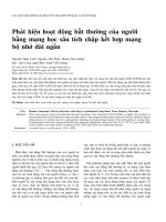
Figure 3.1. A sample 1DCNN configuration with 3 CNN layers and 2
ANN layers.
3.2 Proposed Convolutional Neural Networks
In practice, monitoring infrastructure such as bridges requires long-term
installation of sensors on the structure, continuously transmitting data to data
processing centers. The amount of data to be processed is very large and
sequential over time. However, these networks are not efficient at handling
large datasets or sequential time-series data because they lack memory and the
ability to link data at different time steps. To address these limitations, I
propose an approach based on the combined use of a 1D Convolutional Neural
Network (1DCNN) and a recurrent network, specifically the Long Short-Term
Memory (LSTM) method, to process time-series data obtained from sensors.
This approach aims to monitor structural health, diagnose structural issues, and
avoid the problem of forgetting critical information.
ht
Ct-1


Ct
tanh

ht-1

Ot

it

ft




Ct
tanh



ht

X1dcnn

Figure 3.2. LSTM Model
In 𝑡 condition of LSTM model:
 Output: 𝑐𝑡 ; ℎ𝑡 , we call 𝑐 is cell state, ℎ is hidden state.
 Input: 𝑐𝑡−1 ; ℎ𝑡−1; 𝑋1dcnn . Where 𝑋1dcnn is input of 𝑡
condition of model. 𝑐𝑡−1 ; ℎ𝑡−1 is output of previous layer.
𝑓𝑡 ; 𝑖𝑡 ; 𝑜𝑡 corresponding with forget gate, input gate and output gate.

Forget gate: 𝑓𝑡 = 𝑠(𝑈f ∗ 𝑋1dcnn + 𝑊f ∗ ℎt−1 + 𝑏f )
Input gate: 𝑖𝑡 = 𝑠(𝑈i ∗ 𝑋1dcnn + 𝑊i ∗ ℎt−1 + 𝑏i )
Output gate: 𝑜𝑡 = 𝑠(𝑈o ∗ 𝑋1dcnn + 𝑊o ∗ ℎt−1 + 𝑏o )


12

Comment: 0 < 𝑓𝑡 ; 𝑖𝑡 ; 𝑜𝑡 < 1; 𝑏f ; 𝑏i , 𝑏o are bias coefficient; coefficient
𝑊, 𝑈 is training parameters.
𝑐̃𝑡 =𝑡𝑎𝑛ℎ(𝑈c ∗ 𝑋1dcnn + 𝑊c ∗ ℎt−1 + 𝑏c ),
𝑐𝑡 = 𝑓𝑡 ∗ 𝑐𝑡−1 + 𝑖𝑡 ∗ 𝑐̃𝑡 , The forget gate decides how much to take from
the previous state, and the input gate decides how much to take from the inputs
of previous layers.
ℎ𝑡 =𝑜𝑡 ∗ tanh(𝑐𝑡 ), The output port decides how much to take from the
cell state to become the output of the hidden state. Besides ℎ𝑡 is also used to
calculate the output 𝑦𝑡 for state 𝑡. 𝑐𝑡 Just like a conveyor belt, important
information that needs to be preserved and used later will be carried forward
and used when necessary, which can carry information from a distant point,
thus constituting long-term memory. Therefore, the LSTM model has both
short-term memory and long-term memory.
When data is fed into the network, it is divided into segments of fixed
length. The 1-DCNN layer then extracts local relationships between data
points and their neighbors before passing them to the LSTM layer. Here, longterm dependencies are identified and maintained over time. The output of the
final LSTM cell is flattened and fed into a fully connected layer before being
passed to the output layer with a softmax activation function to provide the
diagnosis of structural damage. This hybrid deep learning algorithm is
implemented with the assistance of open-source TensorFlow code.
CHAPTER 4 APPLICATION OF COMBINED CONVOLUTIONAL
NEURAL NETWORKS WITH SAX-MDWD METHOD FOR
DETECTING VARIOUS TYPES OF DAMAGE IN BRIDGE

MODELS
4.1 Applying Convolutional neural network Combined with SAX-MDWD
Method to Diagnose Defects for a Real Bridge Model
4.1.1 Introduction of the Bridge
To evaluate the effectiveness of the proposed approach, I will use
algorithms to identify the defects of the Z24 bridge based on time-series data.
The Z24 bridge (Figure 4.1) is located in the Bern canton near Solothurn.


13

Figure 4.1 Vertical and horizontal projection of the Z24 bridge [129].
Table 4.1. Cases of detect creation and corresponding labels [130]
Label
0

Date (1998)
04 August

1
2
3
4
5
6
7
8
9
10
11

12
13
14
15

9 August
10 August
12 August
17 August
18 August
19 August
20 August
25 August
26 August
27 August
31 August
02 September
03 September
07 September
08 September

Case of damage
Establish
initial
condition
(undamaged
condition)
Install equipment on the pier
Cut, create defects on the pier (20 mm)
Cut, create defects on the pier (40 mm)

Cut, create defects on the pier (80 mm)
Cut, create defects on the pier (95 mm)
Raise the pier, create a tilting of the foundation
Establish the new undamaged state
Concrete breaking (12 m2)
Concrete breaking (24 m2)
1-meter landslide at the abutment
Create joint damage
Create damage to 2 anchor heads
Create damage to 4 anchor heads
Cut 2 out of 16 cables
Cut 4 out of 16 cables

For each damaged state, 9 setups were conducted to collect data, with
8 setups using 33 sensors and 1 setup using 27 sensors, resulting in a total
of 291 measurement sensors to capture vibrations on the piers (primarily in
the vertical and horizontal directions) and vibrations on the bridge deck.


14

(a)

(b)

(c )

(d)

(e)


(f)

(g)
(h)
Figure 4.2 (a) – (h) Time-series acceleration data at the corresponding
sensors for the damage cases from 1 to 8.
4.1.2 Data processing
To improve the data before using it to train the network, the SAX and
MDWD methods will be applied. Specifically, the process of transforming
continuous time-series data into discrete data using the MDWD method is
performed through the following steps:
- Step 1: Choose a basic wavelet function to analyze the signal.
- Step 2: Perform wavelet transformation on the signal using the chosen
wavelet function. The result of the transformation is the analyzed signal and
the analysis coefficients.
- Step 3: Repeat steps 1 and 2 on the analyzed signal to generate new
wavelet components. These wavelet components will be used to build the
model and analyze the signal.
- Step 4: Repeat steps 1-3 until no more wavelet components are


15

generated or the desired resolution level is achieved.
These steps create a resolution tree for the signal, where each node
corresponds to a wavelet component. Nodes at higher levels correspond to
components with lower frequencies and larger delays, while nodes at lower
levels correspond to components with higher frequencies and smaller delays.
SAX performs signal analysis using the following steps:

 Step 1: Divide the data sequence into segments of equal length.
 Step 2: Calculate the mean value of each segment.
 Step 3: Calculate the standard deviation of each segment.
 Step 4: Transform the value of each segment into a corresponding
symbol using a transformation function.
 Step 5: Create a discrete character string by arranging the symbols
generated from the segments in order.

Figure 4.3 The time-domain acceleration data at a sensor after being
processed using the MDWD and SAX methods.

Figure 4.4 The time-domain acceleration data for the 16 classes after being
processed.
The data, after applying the SAX-MDWD method, undergoes a
transformation from a continuous wave-like form to a time-varying format.


16

This means that the time data will no longer exhibit continuous waveforms but
will be smoothed and focused on areas with significant oscillations. As a result,
the new matrix will have a size of (4000, 5) instead of the original size of
(8000, 5).
4.1.3 Network architecture
Firstly, there is a 1D Convolutional Neural Network (1DCNN) layer
used to extract important features from the model. This CNN layer has the
following characteristics: it uses 128 kernels, and each kernel has a size of 3x3.
After extracting features from the input data, a Long Short-Term Memory
(LSTM) network is employed for learning and classification. The LSTM
network consists of 2 layers, and between these layers, there are Dropout

layers to prevent overfitting, as well as Maxpooling layers to extract essential
features. These design choices help reduce the matrix size, computational load,
and computation time. Finally, the network is flattened with 16 output layers,
each of which is labeled.
4.1.4 Network training and analyze the results
The Adam algorithm was used to train the network with a total of 100
training steps. The network has 8,287,280 parameters that need to be trained.
Figure 4.5 illustrates the convergence of the training and testing processes for
all three methods: 1DCNN, 1DCNN-LSTM, and MDWD-SAX-1DCNNLSTM.
In this thesis, the effectiveness of the proposed methods is also
evaluated using ground truth maps and error matrices. These tools are used to
assess the performance of image processing and computer vision algorithms,
helping to evaluate the model's ability to classify correctly or incorrectly for
each class.

(b)
(a)
Figure 4.5 The convergence of the models: (a) Convergence of the
training process of the three methods, (b) Convergence of the network
evaluation process of the three methods.


17

In addition, to evaluate the model's performance, I used a combination
of methods through "macro avg" and "Loss validate" values.
Table 4.2. Training results of the network using the method
1DCNN-LSTM
MDWD-SAXLayers
1DCNN

1DCNN-LSTM
prec rec f1-sc prec rec f1-sc prec rec f1-sc
0
0.6 0.38 0.46 0.53 0.81 0.64 0.83 0.78 0.64
1
0.51 0.73 0.6 0.69 0.69 0.69 0.85 0.88 0.65
2
0.67 0.76 0.71 0.92 0.79 0.85 0.9 0.93 0.81
3
0.68 0.66 0.67 0.45 0.62 0.53 0.84 0.84 0.69
4
0.71 0.56 0.63 0.85 0.81 0.83 0.87 0.94 0.79
5
0.69 0.67 0.68 0.88 0.85 0.87 0.8 0.89 0.83
6
0.6 0.75 0.67 0.39 0.91 0.55
1
0.88 0.81
7
0.62 0.71 0.67 0.51 0.71 0.6
0.8 0.86 0.65
8
0.67 0.6 0.63 0.93 0.65 0.76 0.81 0.72 0.75
9
0.75 0.8 0.77 0.66 0.83 0.74 0.69 0.97 0.69
10
0.63 0.52 0.57 0.94 0.52 0.67 0.87 0.82 0.7
11
0.56 0.58 0.57 0.76 0.61 0.68 0.72 0.74 0.76
12

0.57 0.74 0.65
1
0.32 0.49 0.76 0.84 0.61
13
0.81 0.65 0.72
1
0.47 0.64 0.83 0.71 0.77
14
0.71 0.53 0.61 0.72 0.41 0.52 0.81 0.66 0.58
15
0.53 0.66 0.59 0.74 0.8 0.77 0.94 0.86 0.72
acc
0.64
0.67
0.83
macavg 0.65 0.64 0.64 0.75 0.68 0.68 0.83 0.83 0.83
Note: pre: precision;
rec: recall;
f1-sc: f1-score

Error matrix: 1DCNN

Error matrix: 1DCNNLSTM

Error matrix: MDWDSAX-1DCNN-LSTM


18

Compare methods

5
0
Accuracy Validate

0.64

0.68

1DCNN

1DCNN-LSTM

0.64

0.68

Loss Validate
3.3
Accuracy Validate

2.1
Loss Validate

0.83
MWD-SAX-…
0.83
0.69

Figure 4.6 Results of the error matrix and accuracy of the networks in the
evaluation step

Comments:
The MDWD-SAX-1DCNN-LSTM model outperforms the 1DCNN
and 1DCNN-LSTM models in terms of Ground truth maps and error matrix
indices, including Recall, Precision, F1-score, and Macro avg.
Figure 4.6 represents the error matrix, where the vertical column
represents the true label, and the horizontal column represents the predicted
label. Higher values on the main diagonal of the error matrix indicate higher
accuracy as the predicted values match the true values.
Figure 4.6 also visually demonstrates the superiority of the MDWDSAX-1DCNN-LSTM method over the 1DCNN and 1DCNN-LSTM methods
in diagnosing structural states from time-series data, with an accuracy rate of
up to 83%, and a Loss Validate value <1, indicating good performance on the
test dataset.
Overall Evaluation:
The deep convolutional neural network combined with the SAXMDWD method has effectively addressed the problem of diagnosing
structures based on time-series data. The training results of the 1DCNN,
1DCNN-LSTM, and MDWD-SAX-1DCNN-LSTM models using time-series
data from the Z24 bridge, as evaluated through Ground truth maps and error
matrices, all show that the MDWD-SAX-1DCNN-LSTM model has
significantly higher accuracy compared to the other two models. The use of
tools to extract and connect data in time-series data has substantially improved
the model's learning outcomes.
In diagnosing the structural integrity of bridges using time-series data,
the uncertainty factor (noise) in the measurement data has a significant impact
on the diagnosis results. The use of methods like MDWD-SAX in data
preprocessing has greatly improved data quality, reduced data complexity, and
increased the reliability of diagnosis results.


19


4.2 Applying a Deep Convolutional Network to damage detection in a
laboratory Bridge
4.2.1 Description
The model is a planar cable-stayed structure with a total of six stay
cables arranged symmetrically in a fan-shaped pattern. The stay cables are
zinc-coated steel cables with a nominal diameter of 2 mm, and they are
connected to the beams through fixed anchors that are directly welded to the
bridge's surface.

Figure 4.7 Laboratory Cable-Stayed Bridge Model
4.2.2 Vibration Measurement Experiment for the Cable-Stayed Bridge
Model
To determine the oscillation characteristics of the cable-stayed bridge
model in the laboratory before reinforcement, a data collection and analysis
system for vibration measurement has been implemented.
The measurement grid is divided into 10 measurement diagrams, each
consisting of 8 acceleration sensors as shown in Figure 4.8 below. There are
two main types of measurement points: reference measurement points and
mobile measurement points. The mobile points in each measurement case are
used to collect the dynamic responses of various points in the measurement
grid. Each measurement diagram will collect measurement data for 20
minutes.

Figure 4.8 Arrangement of
accelerometer

Figure 4.9 Monitoring
measurement data



20

4.2.3 Data Processing
The data has been significantly improved after applying the SAX and
MDWD methods. After applying the SAX-MDWD method, the data has been
transformed from continuous waveforms into time-varying data, meaning that
time no longer varies continuously in waveforms. Instead, it becomes smooth
and focuses only on significant oscillations. The new matrix has a size of
(1500, 8).

Figure 4.10 raw data collected from sensors
The data, before being used for training, will be processed using the
SAX-MDWD method as shown in Figure 4.11.

Figure 4.11 Data after transfer using SAX-MDWD.
4.2.4 Cases of damage
TRƯờNG HợP 3

10 kg
100

250

30 kg
500

10 kg
500

10 kg

500

60

500

10 kg
500

10 kg
500

250

100

3760

Figure 4.12 Case of damage on the cable-stayed bridge model (level 2
damage)


21

4.2.5 Network architecture
The dynamic data obtained from the four damage scenarios (04
scenarios) consist of 1,892 datasets, which were randomly divided into a
training set and a test set, with 70% of the data allocated for training and 30%
for testing. During the training phase, features and labels were provided for all
time series in the training group. Subsequently, the model was constructed to

capture the relationship between the features and class labels.
4.2.6 Results analysis

Figure 4.13 The convergence of the models is shown in the following
figures: (a) Convergence of the training process, (b) Convergence of the
network evaluation process for the models.
Table 4.3. Results of training the network using the method
1DCNN-LSTM
MDWD-SAXLayers
1DCNN
1DCNN-LSTM
prec rec f1-sc prec rec f1-sc prec rec f1-sc
0
0.95 1.00 0.98 0.97 1.00 0.98 0.99
1
0.99
1
0.54 0.92 0.68 0.73 0.37 0.49 0.83 0.59 0.69
2
0.96 0.67 0.79 0.87 0.91 0.89 0.91 0.92 0.91
3
0.96 0.89 0.92 0.82 0.81 0.81 0.85 0.94 0.89
Acc
0.91
0.93
0.95
macavg 0.85 0.87 0.84 0.85 0.77
0.8
0.89 0.86 0.87


Error matrix: 1DCNN

Error matrix: 1DCNN- Error matrix: MDWDLSTM
SAX-1DCNN-LSTM


22

Compare methods
0.91

1
0
Accuracy Validate
Loss Validate

0.92

1DCNN

1DCNN-LSTM

0.91

0.92

0.7
Accuracy Validate

0.6

Loss Validate

0.95
MWD-SAX-…
0.95
0.05

Figure 4.14 Results of the error matrix and accuracy of the networks in the
evaluation step
Comments:
Table 4.3 demonstrates that the MDWD-SAX-1DCNN-LSTM model
outperforms the 1DCNN and 1DCNN-LSTM models significantly in terms of
Ground Truth Maps and error matrices, including Recall, Precision, F1-score,
and Macro avg values. Figure 4.14 illustrates the error matrix, where higher
values on the main diagonal indicate more accurate results because the
predicted values match the actual ones. Specifically, the MDWD-SAX1DCNN-LSTM model achieves the highest matching prediction values
compared to the other two models. Furthermore, Figure 4.14 visually
showcases the superiority of the MDWD-SAX-1DCNN-LSTM method over
the 1DCNN and 1DCNN-LSTM methods in damage detection from timeseries data, with an accuracy rate of up to 95%, and a Loss Validate value
approaching 0, indicating excellent performance on the test dataset.
Evaluation:
The training results of the 1DCNN, 1DCNN-LSTM, and MDWDSAX-1DCNN-LSTM models using time-series data from the cable-stayed
bridge are evaluated based on Ground Truth Maps and error matrices, all of
which show that the MDWD-SAX-1DCNN-LSTM model is significantly
more accurate than the other two models. This suggests the potential
application of the MDWD-SAX-1DCNN-LSTM model in diagnosing
structures in real-life bridge constructions.
The use of methods such as MDWD-SAX in the data preprocessing
phase has considerably improved data quality, reduced data complexity, and
data size, thereby enhancing the reliability of diagnostic results. Ground Truth

Maps and error matrices for the 1DCNN and 1DCNN-LSTM methods when
analyzing time-series data from the cable-stayed bridge in the laboratory are
better than the results from the Z24 bridge measured in the field. This indicates


23

that, under well-controlled conditions that minimize external factors' impact
on measurement results (such as temperature, humidity, measuring equipment,
etc.), the uncertainty characteristics of data can be significantly reduced,
thereby improving the reliability of diagnostics.
CONCLUSIONS AND RECOMMENDATIONS
 Conclusions:
With the aim of proposing a method for non-destructive structural
health monitoring with high accuracy, no alteration of the original physical
characteristics of the structure, minimal cost, and minimal disruption to traffic
flow, while also being suitable for real-time monitoring of bridge structures
and having the potential for application in practical projects, in this
dissertation, I have proposed the use of deep learning networks utilizing timeseries data to diagnose structural damage. Specifically, a deep learning
network combining 1DCNN and LSTM is employed to leverage the strengths
of each method. The 1DCNN network is used to process raw data, filter out
unimportant information, and establish spatial relationships among the data
points. Subsequently, the LSTM network is used to learn, memorize, and
classify the data.
Additionally, to enhance raw data and improve model accuracy, the
SAX and MDWD methods are also proposed for application. Results obtained
from this approach demonstrate high accuracy. The effectiveness of the
proposed method is evaluated through both real bridge Z24 and experimental
models. To compare with the proposed method, the traditional 1DCNN and
1DCNN-LSTM methods are also used in the dissertation. Important

conclusions drawn from the results include:
Time-series data in the structural health monitoring of bridges is
influenced by numerous factors, leading to data with random and uncertain
characteristics and a wide range of distribution. Simultaneously applying the
SAX-MDWD method to time-series data is highly effective in noise reduction
and data improvement before network training.
Simultaneously applying the SAX-MDWD-1DCNN-LSTM method
efficiently exploits data preprocessing and connection, learning data in the
field of diagnosis and structural health monitoring. This enhances the accuracy
of prediction results. Specifically, the accuracy achieved through training and
validating with the SAX-MDWD-1DCNN-LSTM method is 83% for the Z24
bridge and 95% for the laboratory bridge. This accuracy surpasses that of the
traditional 1DCNN and 1DCNN-LSTM methods.