Environmental Background Radiation Monitoring Utilizing Passive Solid Sate Dosimeters
131
dosimeter within a month was estimated tobe about 12μSv. On the other hand, the
averaged self-doses accumulated in the Luxel badge also increases lienarly with increasing
the time except for the bigining of measurement as shown in Fig.14. The value at the
bigining of measurement is different from othe two values. This deviation may be caused by
the exposure to the natural radiation during the transportation of dosimeters to Nagase
Landauer in Tokyo by air. Except for the data point at the bigining of measurement, the
averaged self dose of the Luxel Badge is estimated to be about 9μSv.


Fig. 14. Self-dose of the luxel badge dosimeter. Each data point is averaged over doses of
three Luxel badge units.

.
Fig. 15. Typical γ-ray spectrum obtained from the DIS dosimeter.
0306090
0
20
40
60
average of five luxel badges
Dose reading [Sv]
Time [days]
0 500 1000 1500 2000
0
20
40
60
80

100

Yield [counts/hr/kev]
Energy [keV]
Thorium series
Uranium series
K-40
0 500 1000 1500 2000
0
20
40
60
80
100

Yield [counts/hr/kev]
Energy [keV]
Thorium series
Uranium series
K-40

Environmental Monitoring
132
The origin of the self-dose was identified using high pure Ge semiconductor detector in the
Ogoya underground laboratory. Typical gamma-ray spectrum obtained from the DIS
dosimeter is shown in Fig.15.

dosimeter parts
238
U

(dpm)
210
Pb
(dpm)
232
Th
(dpm)
40
K
(dpm)
DIS
Whole DIS
Label
Spring
Al frame
IC long
IC fat
Battery
1.40

0.88
0.10
1.30
0.83
0.10
2.00



1.50

0.85
22.0
0.38

0.75
Luxel
Al
2
O
3
crystal
Ag filter
Sn filter
2.00

0.07


1.70
1.50

0.04


5.53
Table 2. Identificated radioactive nuclides contained in each personal dosimeters.


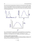
Fig. 16. Measured environmental radiation dose using the GD-450 glass dosimeter in seven
points such as Tsurugi-machi (◆), Tatsunokuchi (●), outside of Mt.Shishiku (■), inside of

house in Mt.Shishiku, (▲), outside of Ogoya Mines (◇), Inside of Ogoya Mines (○) and
rooftop of Ishikawa Prefecture Institute of Public health and Environmental Science (□). in
Ishikawa prefecture. The measurements of environmental radiation dose were carried out
from March in 2008 to August 2009.
The sveral peaks under 1000 keV correspond to nuclides of
232
Th and
238
U series. The
40
K
peak with the energy of 1460 eV has been also detected. Measured parts and identified
0
0.02
0.04
0.06
0.08
0.1
0.12
0.14
0.16
345678910111212345678
MEASUREMENTS [mGy]
TIME [month]

Environmental Background Radiation Monitoring Utilizing Passive Solid Sate Dosimeters
133
radioactive nuclies are listed in Table 2. The
40
K,

232
Th and
238
U have been contained in
almost all dosimeters. So, it is difined that the self-dose of each dosimeter for a month is
about 10-15μSv. Data was, therefore, compensated for each dosimeter which based on the
sel-dose rate of about 12μSv/month.
The environmental backgroung radiation dose at 7 points for one month were monitored
using the glass dosimeter (GD-450) as well as the Luxel badge and the DIS dosimeters. The
monitoring results of typical environmental background radiation dose in gray (Gy) as the
absorbed dose using the GD-450 from March in 2008 to August 2009 are shown in Fig.16 for
7 points in Ishikawa prefecture.
Although natural background radiation doses with the GD-450 dosimeter at each point in
Ishikawa prefecture were significantly different, the standard deviations were very small.
Although the values were a little bit different between the GD-450 glass dosimeter and the
Luxel badge (OSL dosimeter), the tendencies of the environmental dose at each point were
very similar as shown in Fig.17. The higher dose at point B (Tatsunokuchi) than at other
points is due to the use of radioisotopes at the Lowere Level Radiation laboratory in
Kanazawa University. Morever, the values of the GD-450 dosimeter and the DIS dosimeter
were very close and there was no significant difference between them as shown Fig.18. We
have made the comparison of different types of RPL glass dosimeters such as Type: GD-450
for personal dosimeter and Type:SC-1 for enviromental monitoring, which were supplied
from Chiyoda Technol Corp, as shown in Fig.19. It was found that there is no significant
difference at each points.


Fig. 17. Dose response at each point in Ishikawa prefecture (A: Tsurugi-machi, B:
Tatsunokuchi, C: Inside of house of Mt. Shishiku, D: Outside of Mt. shishiku, E: Inside of
Ogoya Mines, F: Outside of Ogoya Mines, G: Public health and Environmental Science)
using GD-450 (blue bars) or Luxel badge (orange bars) dosimeters.

0
0.02
0.04
0.06
0.08
0.1
0.12
0.14
0.16
0.18
ABCDE FG
ｍSv
GD-450
Luxel

Environmental Monitoring
134

Fig. 18. Dose response at each point in Ishikawa prefecture (A: Tsurugi-machi, B:
Tatsunokuchi, C: Inside of house of Mt. Shishiku, D: Outside of Mt. shishiku, E: Inside of
Ogoya Mines, F: Outside of Ogoya Mines, G: Public health and Environmental Science)
using GD-450 (blue bars) or DIS (purple bars) dosimeters. There is no data at G for DIS.


Fig. 19. Dose response at each point in Ishikawa prefecture (A: Tsurugi-machi, B:
Tatsunokuchi, C: Inside of house of Mt. Shishiku, D: Outside of Mt. shishiku, E: Inside of
Ogoya Mines, F: Outside of Ogoya Mines, G: Public health and Environmental Science)
using GD-450 (blue bars) or SC-1 (green line) dosimeters. The unit of the GD-45 and SC-1
are represented by mSv and mGy, respectively.
0

0.02
0.04
0.06
0.08
0.1
0.12
ABCDEFG
mSv
GD-450
DIS
0
0.02
0.04
0.06
0.08
0.1
0.12
ABCDEFG
ｍSv
0
0.01
0.02
0.03
0.04
0.05
0.06
0.07
0.08
0.09
ｍGy

GD-450
SC-1

Environmental Background Radiation Monitoring Utilizing Passive Solid Sate Dosimeters
135
From the results as described above, Monitoring environmental natural background
radiation dose with a personal GD-450 seems to be feasible and consequently, one can say
that the GD-450 dosimeter can be suitable for monitoring environmental natural
background radiaiton dose.
5. Summary
Environmental natural background radiation dose values at 7 points in Ishikawa prefecture
determined using the personal glass dosimeter, type GD-450 were compared with these
determined some other personal dosimeters such as DIS dosimeter utilizing a MOSFET with
an ioniization chamber and OSL dosimeter, Luxel budge, utilizing OSL phenomenon in
Al
2
O
3
:C phosphor. The actual dose values were different from each other, however, the
tendency of each dose at each point were very similar. It can be said that the personal glass
dosimeter will be very useful for not only monitoring personal dose but also monitoring
natural background radiation dose.
6. Acknowledgements
The author wish to thank Dr.Yamamoto, Directer of the Research Center of Chiyoda Technol
Corp. for his fruitful discussion and Dr.Kobayashi of Nagase Landauer Co. Ltd, Dr.
Kakimoto of Ishikawa Prefecture Institute of Public health and Environment Science for
their excellent assistance.
The work on the environmental natural background radiation monitoring using solid state
passive dosimeters was partially supported by the foundation for Open-Research Center
Program from the Ministry of Education, Culture, Sport, Science and Technology of Japan

and Chiyoda Technol Corp.
7. References
Kobayashi, I, (2004), The detection of the Environmental radiation for DIS and Luxel badge,
Ionizing Radiation, Vol.30, pp.33-43.
Koyama, S., Miyamoto, Y., Fujiwara, A., Kobayashi, H., Ajisawa, K., Komori, H., Takei, Y.,
Nanto, H., Kurobori, T., Kakimoto, H., Sakakura, M., Shimotsuma, Y., Miura, K.,
Hirao, K. And Yamamoto, T., (2010), Environmental Radiation Monitoring
Utilizing Solid State Dosimeters, Sensors and Materials, Vol.22, No.7, 377-385.
Miyamoto, Y., Takei, Y., Nanto, H., Kurobori, T., Konnai, A., Yanagida, T., Yoshikawa, A.,
Shimotsuma, T., Sakakura, M., Miura, K., Hirao, K., Nagashima, Y. and Yamamoto,
T., (2011), Radiophotoluminescence from Silver-Doped phosphate Glass, Radiation
Measurements, in press.
Murata, Y., Yamamoto, M. and Komura, K., (2002), Determination of low-level
54
Mn in soils
by ultra low-background gamma-ray spectrometry after radiochemical separation,
J. Radiational Nucl. Chem, Vol.254, No.2, pp.249-257.
Hsu, S.M., Yeh, S.H., Lin,M.S. and Chen, W.L., (2006), Comparison on characteristics of
radiophotoluminescent glass dosimeters and thermoluminescent dosimeters,
Radiation Protection Dosimetry, 119, 327-331.
Nanto.H, (1998), Photostimulated Luminescence in Insulators and Semiconductors,
Radiation Effects & Defects in Solids, Vol.146, pp.311-321.

Environmental Monitoring
136
Nanto, H., (1999), Physics of photosimulable phosphor materials, Ionizing Radiaiton, Vol.
25, No.2, pp.9-24. (in Japanese)
Nanto, H., Takei, Y., Nishimura, A., Nankano, Y., Shouji, T., Yanagida, T., Kasai, S., (2006),
Novel X-ray Imaging Sensor Using Cs:Br:Eu Phosphor for Computed Radiography,
Proc. of SPIE, Vol. 6142, pp.6142w-1-6142w9.

Nanto, H., (2011), Basic princple of accumulation-type personal dosimeter for ionizing
radiation and its application, Ionizing Radiation, Vol.37, No.2, pp.3-9.
Ranogajec-Komor, M., Knezevic, Z., Miljanic, S. And Velic, B., (2008), Characteristics of
radiophotoluminescent dosimeters for environmental monitoring, Radiation
measurements, Vol.43, 392-396.
Saez-Vergara, J.C., (1999), Practical Aspects on The Implementation of LiF:Mg, Cu, P in
Routine Environmental Monitoring Program, Radiation Protection Dosimetry,
Vol.1-4, pp.237-244.
Sarai, A., Kurata, N., Kamijo, K., Kubota, N., Takei, Y., Nanto, H., Kobayashi, I., Komori, H.,
and Komura, K., (2004), Detection of self-dose from an OSL dosimeter and a DIS
dosimeter for environmental radiation monitoring, J. Nuclear Science and
Technology, Suppl. 4, pp.474-477.
Wernli, C., (1998), Direct ion strage dosimeters for individual monitoring, Radiation
Protection Dosimetry, Vol.77, pp.253-259.
9
PILS: Low-Cost Water-Level Monitoring
Samuel Russ, Bret Webb, Jon Holifield and Justin Walker
University of South Alabama
United States of America
1. Introduction
The estuarine environment is important both to global ecology and to human economy.
Estuaries are the place where freshwater meets saltwater, and so they typically contain a
bounty of marine species, and are essential to the life cycle of many marine organisms. For
similar reasons, they often contain sea ports and carry commerce of great value.
In order to study estuaries in more detail, we have developed two sets of low-cost sensors
using off-the-shelf technology combined with innovative new low-cost circuits. The first,
nicknamed “Jag Ski”, is a highly mobile water craft for navigating estuarine and littoral
areas and providing real-time data. The second, named “PILS”, is a network of stationary
sensors for making long-term water-level measurements. This paper describes the
construction of both, along with actual measurements.

2. Survey of literature
Sensing the environment can be carried out through remote measurements (e.g. satellites
(Villa & Gianietto, 2006)) and through in situ measurements (e.g. wireless sensor networks
(O’Flyrm et al., 2007; Thosteson et al., 2009)). Both have been demonstrated successfully as
means of measuring characteristics of water.
An example of one real-time water-sensor architecture is the Land/Ocean Biogeochemical
Observatory (LOBO) system developed by Satlantic and the Monterrey Bay Aquarium
Research Institute (MBARI) (Comeau et al., 2007; Jannasch et al., 2008) and has been
installed in the field (Sanibel-Captiva Conservation Foundation, 2009). Others include the
Ocean Observation Initiative (OOI) (Frolov et al., 2008; National Research Council, 2003;
U.S. Commission on Ocean Policy, 2004), NOAA tide gauges for storm surge (Luther et al.,
2007), and sonar-based water-level measurements (Silva et al., 2008). Specific to
environmental monitoring in the coastal ocean, mobile field assets typically include
profiling floats (Roemmich et al., 2004), autonomous underwater vehicles (AUVs) (Rudnick
et al., 2004), and unmanned underwater vehicles (UUVs) (Freitag et al., 1998; Frye et al.,
2001).
This work is in line with these earlier systems. We have adapted the mobile sensor platform
to a highly maneuverable manned platform to navigate shallow-water areas proficiently.
The sensor network is designed for relatively low cost and for unattended measurements. It
also contains novel sensors for pressure and salinity.

Environmental Monitoring

138
This work is motivated by the fact that computer models of estuaries need refinement. For
example, there is disagreement whether wind forcing or river discharge dominates the
dynamics of Mobile Bay (Schroeder & Wiseman, 1986; Kim et al., 2008). Data obtained using
the sensors will be used to parameterize a linear approximation of a static momentum
balance of the estuary (Van Dorn, 1953) to improve simulation and forecasting accuracy.
3. Real-time monitoring: Jag Ski

The University of South Alabama Jag Ski is a three-person Kawasaki Ultra LX personal
watercraft (PWC) equipped with state of the art instrumentation developed by YSI,
Incorporated, SonTek, VarTech Systems, and others (Fig. 1). In addition to the PWC, a
Kawasaki Mule 3010 four-wheel drive utility vehicle can be used for launching and retrieval
when a proper boat launch is not available. The Jag Ski contains an onboard small-form PC
running the Windows XP operating system, a foldable waterproof keyboard, a fully
submersible touch screen LCD display, and four dry-cell 18 amp hour, 12 volt marine
batteries to supply enough dedicated power for twelve to fourteen hours of data collection.
The PC, power supply, and other assorted equipment are housed in waterproof cases with
internal foam padding. All external cabling and bulkhead connectors are fully submersible.
Experience has demonstrated that items labeled water resistant and waterproof offer little
protection in the corrosive, marine environment.


Fig. 1. The South Alabama Jag Ski and 4x4 towing vehicle.
The use of PWCs for collecting hydrography is not a new idea. There are numerous
examples of PWC systems around the country (and world). Some of the earlier successful
applications are discussed in (Dugan et al., 1999; Dugan et al., 2001; MacMahan, 2001; Puleo
et al., 2003). The PWC has also successfully been used for larval fish sampling in shallow
waters (Strydom, 2007). More recently, however, Hampson et al. (2011) have demonstrated
the skill of using a kayak as a surveying platform for still shallower survey applications.
What perhaps makes the Jag Ski so unique in the context of PWC hydrographic data
collection systems is its suite of instrumentation. Prior to the Jag Ski, the use of the PWC has
been mostly limited to bathymetric surveys in nearshore waters. While it certainly has its
limitations, the ability of the PWC to traverse the surfzone in hydrographic surveying
cannot be rivaled by most traditional vessels. The addition of a PWC to one’s hydrographic
surveying deployment provides a very good overlap between land-based surveys and those
conducted in deeper waters using traditional watercraft. The Jag Ski, however, was

PILS: Low-Cost Water-Level Monitoring


139
developed to meet broader goals and objectives in the area of coastal, water resources, and
environmental engineering.
The Jag Ski contains a SonTek/YSI RiverSurveyor M9 Acoustic Doppler Current Profiler
(ADCP) with an integrated Real Time Kinematic Differential Global Positioning System
(RTK DGPS) for georeferenced measurements (Fig. 2). The M9 ADCP has a profiling range
of 6 cm to 40 m, and is capable of measuring velocity magnitudes up to 20 m/s. The
resolution of the velocity measurements is as low as 0.001 m/s, and vertical bin sizes can be
as small as 2 cm, or as large as 4 m. The horizontal resolution of the samples is a function of
the reported sample rate (generally 1 Hz) and vessel speed (preferably equal to or less than
the water velocity). A nominal speed of 1 – 2 m/s is maintained when using the M9 ADCP
on the Jag Ski, so a typical horizontal resolution is, accordingly, 1 – 2 m.


Fig. 2. SonTek/YSI RiverSurveyor M9 ADCP and RTK DGPS base station.
The M9 ADCP contains a dedicated 500 KHz vertical beam for depth measurements and
bottom tracking, four slanted 1 MHz beams for sampling in deeper water, and four
slanted 3 MHz beams for sampling in shallower waters (Fig. 3). This dual-frequency
functionality is unique in the ADCP market, and along with its integrated GPS system for
vessel-corrected measurements to account for the moving reference frame, makes it
attractive for applications in Mobile Bay (Fig. 4). The bay is a broad, mostly shallow
(< 4 m), drowned river mouth estuary that is incised by a navigation channel dredged to a
maintenance depth of about 15 m. The depth of the channel in the main entrance to
Mobile Bay can reach 20 m or more, and is flanked to the west by a broad, shallow area
with depths less than 3 m. The dual frequency M9 ADCP performs well when
transitioning between the two extremes.
Aside from the technical capabilities of the RiverSurveyor M9 ADCP, the instrument comes
with a well-developed, integrated software package for setup and data collection. The
RiverSurveyor Live (RSL) software is loaded on the onboard PC, and is fully interactive

using the touch screen LCD display. Some very helpful features of the software include
dynamic icons that quickly report the status of various systems, like GPS and bottom

Environmental Monitoring

140
tracking, the ability to see a real-time estimate of discharge, and the integrated GIS shapefile
functionality for easy navigation and spatial awareness.


Fig. 3. SonTek/YSI RiverSurveyor M9 ADCP head.


Fig. 4. Terra/MODIS imagery of Mobile Bay taken November 8, 2002. Image courtesy:
NASA Visible Earth.
The initial research focus for the Jag Ski was fulfilled with the integration of the
RiverSurveyor M9 ADCP. That one piece of equipment provides the capability to perform
detailed beach profile surveys, detect and image scour holes near bridge foundations, and
measure the spatial variability and magnitude of coastal and nearshore currents, as well as
riverine flows. And as preparations were being made in April 2010 for upcoming field
experiments in coastal Alabama during the months May – August, the explosion and
subsequent sinking of the Deepwater Horizon drilling platform later that month unveiled a
new, and unexpected, application for the Jag Ski: environmental monitoring.
The National Science Foundation (NSF) issued a number of awards for research, instrument
acquisition, and instrument development related to the 2010 Gulf Oil Spill through their
RAPID program in the months following the initial explosion and sinking of the platform.
The Jag Ski received one such award, issued through the NSF Major Research
Instrumentation program. The purpose of the award was to purchase an instrument that
could be used to measure near-surface water quality parameters, as well as crude oil and
refined fuels, in Alabama’s coastal waters. The result is a rather unique piece of equipment


PILS: Low-Cost Water-Level Monitoring

141
produced by YSI, Inc. called a Portable SeaKeeper 1500 (Fig. 5). The Portable SeaKeeper, or
PSK, is a scaled-down version of the SeaKeeper 1000 systems that are deployed on nearly 50
different vessels of opportunity around the world. Some vessels are used for research,
others are operational ferries, and still others are private yachts. Each of these vessels
contributes data and research to the International SeaKeepers Society, and now the Jag Ski
does, too (Fig. 6).


Fig. 5. The YSI Portable SeaKeeper 1500 mounted on the stern of the Jag Ski.


Fig. 6. Initial testing of the YSI PSK on a local river.

Environmental Monitoring

142
The PSK contains an YSI 6600v2 sonde, a Turner Designs C3 submersible fluorometer, a
Thrane & Thrane Sailor Mini-C vessel monitoring system, a diaphragm pump, and a
dedicated small-form PC running the Windows XP operating system (Fig. 7). The PSK
continuously draws near-surface water by way of a ram intake and pump, routes it
through a manifold, and then to flow chambers attached to the YSI 6600v2 and Turner
Designs C3. The YSI sonde measures temperature, specific conductivity (salinity), pH,
turbidity, dissolved oxygen, and chlorophyll. The Turner Designs fluorometer measures
chromophoric dissolved organic matter (CDOM), crude oil, and refined fuels relative to a
calibration standard or deionized water. The Sailor Mini-C contains a 12-channel GPS
receiver, and Inmarsat-C antenna and transceiver, which provide vessel positioning and

data telemetry to the SeaKeepers online data repository. The PSK currently reports
samples at 0.0833 Hz, but this value can be increased or decreased by the user. In the
coming months, an R.M. Young meteorological station is being added to the Jag Ski and
integrated with the PSK system. The meteorological station will provide continuous
underway measurements of wind speed and direction, air temperature, relative humidity,
and barometric pressure.
If the suite of sensors and measurement capabilities of the PSK are not impressive enough,
then perhaps the ability to collect this data while cruising at 40 knots is! The custom-
designed ram intake and diaphragm pump allow for a continuous stream of water to be
drawn from the near surface (about 10 cm below the surface) regardless of the speed, and
the center-point allows it to track with the vessel when turning at high speed (Fig. 8).
The YSI PSK system is playing an important role in the yearlong BP-funded Gulf Research
Initiative program that seeks to evaluate the impacts of the Deepwater Horizon events on
Alabama’s coastal resources. With the YSI PSK system, the first synoptic survey of Mobile
Bay’s near-surface characteristics will be achieved in the summer of 2011. The ability to map
a majority of the bay’s surface in less than a quarter tidal cycle provides tremendous
opportunities for practical, applied research ranging from coastal and estuarine
hydrodynamics to watershed management. In terms of the Gulf Research Initiative, the PSK
data will be used in combination with the M9 ADCP data to describe transport pathways
that are effective in communicating constituent material from the Alabama shelf, through
Mobile Bay, and to the Mobile-Tensaw river delta. A number of field experiments are
planned for late summer and early fall of 2011 that will isolate the seasonal (i.e. wet/dry,
warm/cool, windy/calm) and tidal (i.e. spring/neap) variability of Mobile Bay’s dynamics.
Beyond academic research, the ability of the PSK to rapidly measure large spatial
distributions of dissolved oxygen, turbidity, chlorophyll, and CDOM make it suitable for a
number of environmental applications, from tracking and mapping harmful algal blooms
(HAB’s) to the measurement and analysis of Total Maximum Daily Loads (TMDL) in the
Mobile Bay watershed.
While the YSI PSK 1500 has impressive capabilities, its sampling is limited to one location in
the water column for the duration of a survey. It is possible to lower the PSK intake to

sample from a different portion of the water column, but this is something that would limit
the speed of the vessel. Since an estuary like Mobile Bay can be highly stratified at times, the
near-surface PSK data may not necessarily be representative of the entire water column;
therefore, CTD casts are performed from the PWC at predetermined locations to evaluate
stratification at the time of the survey. The idea of performing CTD casts (conductivity-
temperature-depth) from a PWC was not practical until the recent release of the YSI
CastAway CTD profiler (Fig. 9).

PILS: Low-Cost Water-Level Monitoring

143


Fig. 7. Internal components of the YSI PSK system. The YSI sonde is on the right, the Turner
Designs fluorometer is the black cylinder, the flow manifold is on the left, and the onboard
PC is at the bottom. The diaphragm pump is hidden behind the PC.


Fig. 8. The custom-designed center-point swivel and ram intake for the YSI PSK.

Environmental Monitoring

144

Fig. 9. The YSI CastAway CTD profiler and magnetic stylus.
The CastAway CTD has an internal GPS that logs the time and location of each cast. The
user-interface is simple and intuitive, and every operation is controlled using a magnetic
stylus. Data offloads are accomplished through a Bluetooth connection between the device
and a PC running the CastAway software. The CastAway is ultra-portable, making it
suitable for deployment from the Jag Ski.

3.1 Case study – Mobile Bay field experiment
A small field experiment conducted on April 1, 2011 in Mobile Bay (Fig. 10) demonstrates
the full capabilities of the Jag Ski described previously. The objective of the experiment was
to perform a complete hydrographic survey of the lower portion of Mobile Bay during neap
tide conditions. An ADCP transect was collected at each of Mobile Bay’s primary
connections to surrounding water bodies, continuous underway sampling of near-surface
waters was performed, and two CTD casts were obtained.


Fig. 10. Overview of study area and locations of CTD profiles at Mobile Pass on April 1, 2011.

PILS: Low-Cost Water-Level Monitoring

145
The survey took place from 0800 – 1200 hours EDT on Friday, April 1, 2011, beginning and
ending at Dauphin Island, Alabama. The tides during the field experiment were in neap,
with little variation. Although the survey took place on a falling portion of the tide, the tide
was flooding at Mobile Pass and Pass aux Herons throughout the survey, suggesting that
the tide propagates into Mobile Bay as a standing wave. A notable departure from the
oscillatory tidal signal was evident three days prior to the survey.
Measurements of wind speed and direction, taken from NOAA CO-OPS station number
8735180, for a period four days prior to and during the experiment were analyzed to
determine the effects of meteorological forcing on estuarine flows. Conditions during the
survey were generally calm, with wind speeds of 3 – 6 m/s out of the west and northwest.
Wind speeds were considerably higher three days prior to the survey, and out of the east and
southeast. The combination of higher winds and an easterly direction may explain the non-
tidal behavior mentioned previously, where Ekman convergence may have produced setup
along the Alabama coast. The wind forcing during the study period, however, was weak.
Preliminary (raw) ADCP data at Mobile Pass is shown in Fig. 11. The top panel of Fig. 11
shows the bathymetry between Dauphin Island and Fort Morgan. The middle panel is an

overview of the survey location and track, where the green areas denote land. The lower
panel of Fig. 11 shows the distribution of velocity magnitude (m/s) across Mobile Pass,
where cooler colors denote slow-moving water, and warm colors denote faster-moving
water (about 1 m/s). Note that the highest magnitudes occur in the deeper portion of the
channel. The total discharge across the pass is nearly 10,400 m
3
/s.



Fig. 11. Bathymetry and velocity magnitude at Mobile Pass for April 1, 2011 during the
period 0800 – 0900 hours EDT. The estimated total discharge across the transect was
10,400 m
3
/s.

Environmental Monitoring

146
Measurements of flow and bathymetry were also collected at Pass aux Herons, to the
west of the Dauphin Island Bridge. The preliminary (raw) ADCP data for Pass aux Herons
is provided in Fig. 12. The orientation of the plots in Fig. 12 is slightly different than Fig.
11, where north is on the right side of the page in the upper and lower panels. Similar to
the flooding tide at Mobile Pass, the strongest flows are confined to the navigation
channel and Grant’s Pass (just north of the channel), and attain a magnitude of about
1.2 m/s. Unlike Mobile Pass, however, very strong flows are distributed equally over the
water column in the channel and pass. The estimated discharge across this transect
was 3,300 m
3
/s, or about 25% of the total volume flooding into Mobile Bay during the

period 0800 – 1100 hours EDT, April 1, 2011, when considering the discharge across
Mobile Pass.




Fig. 12. Bathymetry and velocity magnitude at Pass aux Herons on April 1, 2011 from
1015 – 1100 hours EDT. The estimated total discharge across the transect was 3,300 m
3
/s.
An overview of the study area and survey-level view of the CTD locations is shown in Fig.
10. The orange and black dots denote the western and eastern locations of CTD profiles,
respectively, provided in Fig. 13. These colors correspond to the orange and black lines in
Fig. 13. The vertical profiles of temperature, salinity, and density show only a slight
variation over depth near the navigation channel. The CTD cast closest to Dauphin Island
suggests a more stratified condition in this portion of the pass, with a notable halocline and
pycnocline about 1 to 1.5 m above the bed. Note, however, the very low values of salinity
and density at each CTD cast location, even during the flood tide, suggesting the presence of
a strong freshwater front.

PILS: Low-Cost Water-Level Monitoring

147

Fig. 13. Vertical profiles of temperature, salinity, and density for two locations at Mobile
Pass on April 1, 2011. The orange line represents the western-most CTD cast, while the black
line denotes the CTD cast closer to the navigation channel.
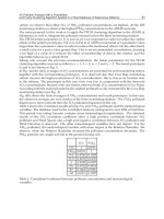
Near-surface water characteristics are shown in Fig. 14, where the vessel track is coincident
with the spatial distribution of data points. Note the agreement of near-surface temperature
and salinity in Fig. 14 with the corresponding values from the CTD profiles shown in Fig.

13. The low salinity environment detected by the CTD profiling is widespread, even on the
flooding tide, extending across Mobile Pass and northward into the bay. Values of
temperature and salinity entering Mobile Bay from Mississippi Sound across Pass aux
Herons, however, were higher. The spatial distributions of near-surface pH, chlorophyll,
turbidity, dissolved oxygen, refined fuels, crude oil, and chromophoric dissolved organic
matter (CDOM) are also shown in Fig. 14, and their magnitudes and units are specified in
each panel. In general, the pH ranged from 7 to 8, the concentration of chlorophyll was low,
the turbidity was low, and the dissolved oxygen content was high.
Measurements of refined fuel, crude oil, and CDOM shown in Fig. 14 are made in relative
fluorescent units (RFU). For reference, deionized water would have an RFU value of zero,
and is commonly used as a calibration standard when the measurement of specific volatile
organic compounds cannot be anticipated a priori. More simply put, the use of the RFU scale
yields a broad-spectrum measurement of the presence of organic compounds in general. In
order to measure the volumetric concentration of fuel or crude oil, a corresponding standard
would have to be used in the calibration of the instrument. What can be inferred from Fig.
14, though, is that there was a strong return in the measurements of crude oil and CDOM
across Mobile Pass and northward into the bay, with much lower values at Pass aux Herons.
By comparison, the presence of refined fuels was much weaker, with the exception of one
location north of Little Dauphine Island along the centerline of the navigation channel.

Environmental Monitoring

148

Fig. 14. Near-surface temperature, salinity, pH, chlorophyll, turbidity, dissolved oxygen,
refined fuels, crude oil, and chromophoric dissolved organic matter on April 1, 2011. The black
line represents the shorelines of south Mobile County, Dauphin Island, and Fort Morgan
peninsula. The spatial location of the data points shows the vessel track during the survey.
With each successive deployment, the Jag Ski is demonstrating its utility and reliability as a
suitable data collection platform in Mobile Bay’s shallow waters. Many have asked why a

PWC was chosen instead of a small boat, which might provide more protection while on the
water. The simple answer is that in terms of access and ease of use, the PWC cannot be rivaled.
The PWC is easy to launch and retrieve, it can be towed by just about any vehicle, and it is
much more agile traversing the surfzone than any other craft on the water. In terms of weather
conditions, the limitations of the ADCP tend to be more restrictive than the capabilities of the
PWC. It is difficult to obtain quality ADCP measurements when the waves are 1 m or greater,
but one can still safely operate the PWC in those conditions. Finally, the cost of the PWC is
much less than a vessel of any significant size.
4. In-situ monitoring: PILS
An effective complement to a mobile platform is a system of low-cost fixed sensors. The goal
of the Pressure-Induced Water-Level Sensor (PILS) is to monitor water level over a long

PILS: Low-Cost Water-Level Monitoring

149
period of time, so that it can be correlated to wind, tides, and freshwater flow. In order to be
able to deploy a large number of sensors, the PILS unit needs to be low-cost. The units are
submerged and estimate water level by measuring water pressure. However, water density
varies with temperature and salinity, and so, to measure water depth, temperature and
salinity also need to be measured. (The salinity cannot be assumed since, in the brackish
estuarine environment, it varies widely.)
Measurement of temperature is straightforward, as integrated temperature sensors are
readily commercially available. Since the unit will make intermittent measurements with
very low power dissipation, the temperature of the interior of the sensor will be extremely
close to that of ambient, and so the temperature sensor will indicate the temperature of the
surrounding water. A Maxim DS1621 temperature sensor was chosen; it uses the
microprocessor’s I
2
C bus to communicate.
Measurement of pressure is more complicated because the sensor must be able to register

changes in pressure. Thus the pressure sensor must lie outside the waterproof housing. A
housing for a commercially available low-cost pressure sensor has been developed and
tested, and is described in detail below in section 5.
Measurement of salinity is considerably more complicated because of the ionic nature of
seawater. The development of a low-cost pressure sensor is detailed below in section 6.
To make measurements over an extended period of time, the system was designed with
flash memory to record readings, a real-time clock to simplify the control of periodic
measurements, and a low-cost microcontroller. An Atmel ATMega168 microcontroller was
selected along with a serial flash memory and a Maxim DS1337 real-time clock chip. A block
diagram of the PILS system is shown below in Fig. 15.

Microprocessor
Atmel ATMega168
Flash
Memory
Digital Pot. H-Bridge Bridge Output
Salinity Sensor
Pressure
Sensor
Temp.
Sensor
Real-Time
Clock
SPI I
2
CA/DAnalog Comparator InterruptGen Purpose I/O

Fig. 15. Block diagram of PILS unit, including its sensor package.
Not counting resistors, capacitors, or a circuit board, the devices listed above have a total
cost below $30.

The flash memory is a Winbond W25X80 serial flash. It operates on the microcontroller’s SPI
bus and has 8 Megabits (1 Megabyte) capacity.
In the process of programming the driver for the flash chip, special considerations were
needed to account for the hardware limitations. The problems revolve around the 256 byte
page buffer used for programming the flash. If a segment of data was larger than 256 bytes
it needed to be broken down into smaller segments. Another, more complicated problem is
that the buffer corresponds to a 256-byte page of actual flash (Winbond, 2007). Therefore, if
it is necessary to start a segment of data in the middle of a 256 page, it is necessary to end
the segment at the end of that page, program the page, and then finish the segment on the
next page. These issues were addressed in the design of the flash drivers, and storage of
data structures to flash has been tested.
A data structure is needed to store the measurements in flash in an ordered fashion so that
they may be retrieved later on. The system must store the time, temperature, pressure, and

Environmental Monitoring

150
salinity. The time requires 7 bytes of space for a detailed time stamp. The temperature needs
2 bytes. Sixty pressure measurements are needed (to provide a sample of wave action). With
each pressure measurement using 2 bytes, 120 bytes are needed for the wave and water
level data. Finally, 2 bytes are needed for the salinity measurements.
A linked list was selected for storage of the data in the flash memory. Each data structure
has a 3 byte pointer at the end which gives the address of the next data structure. This
allows the software to traverse the list when outputting the data with ease. Additionally, the
microprocessor keeps track of where the next set of data must be placed or the tail of the
linked list. This allows for quick storing speed without having to read from the flash. A
more complicated data structure is not needed because the only time the data is accessed is
when the list is parsed at microprocessor start-up. Thus direct access to the data in the
middle of the flash is not needed, only the starting address for output of data and the
address of the next available slot for storage of new data.

The clock chip was selected to simplify the process of taking periodic measurements and
“sleeping” between measurements. The chip uses a 32.768 kHz “tuning fork” crystal, similar
to those in wristwatches, to keep time, and has programmable alarms. When the alarm time
is reached, the chip asserts an interrupt that “wakes up” the microcontroller. Thus the entire
measurement sequence is inside an interrupt service routine.
5. Low-cost pressure sensor
Since the goal of the PILS project is the development of a low-cost deployable sensor, the
design proceeded with a low-cost MEMS-based pressure sensor. A Freescale MPXM2010GS
sensor was selected. It measures gauge pressure and has a dynamic range of 10,000 kPa
(roughly 1 m of water depth). The limited dynamic range was selected for initial tests due to
earlier difficulties with sensors having higher dynamic range.
To amplify the signal coming out of the pressure sensor, an op-amp circuit was designed
based on an application note from Freescale (Clifford, 2006). Interestingly, the application
note explained how to sense water depth in a washing machine. The output of the op-amp
circuit was routed into the A/D converter of an Atmel ATMega 168 microcontroller and
software was written to obtain samples periodically from the sensor.
The sensor was connected to a piece of tubing with a balloon on the end, so that the
prototype unit did not need to be submerged. The balloon was submerged in the wave tank
facility at the University of South Alabama, and six seconds of data were obtained. Pictures
of the unit under test and of the data are shown below in Figs. 16 and 17.


Fig. 16. Pressure sensor. Note balloon and tubing.

PILS: Low-Cost Water-Level Monitoring

151

Fig. 17. A/D converter data from the ATMega168. The sample period was 100 ms.
The pressure-sensor data not only measures pressure but also is accurate enough (at the

relatively shallow depth of the test) to indicate wave action. Thus the PILS unit will measure
not only water level but also wave height.
6. Novel salinity sensor
As noted above, the ability to measure salinity is necessary in order to measure water
density and thereby convert a pressure reading to a measurement of water depth. Water
salinity can be estimated by measuring the conductivity of a cell of known geometry (that is,
the conductance measured between a pair of calibrated electrodes) and then compensating
for temperature.
To measure the bulk conductivity of a sample, a set of electrodes of known geometry is
used. The set is calibrated ahead of time using solutions of known salinity. The process can
be described mathematically as follows.
First, it is well-known that the resistance, R, of a substance can be found as follows
R=

l/A (1)
where

is the bulk resistivity of the material, l is the length of the material (in this case, the
spacing between the electrodes and therefore the length of the water being measured), and A
is the area of the material (in this case, similarly, the area of the electrodes). l/A, then, is the cell
constant C which has units of reciprocal-length.  is an intrinsic property of the material being
measured and C is an intrinsic property of the set of electrodes. (Note that, in this article, we
use the terms resistance and conductance to refer to a measured property of the material being
tested and the terms resistivity and conductivity to refer to the intrinsic property of the material
being tested. The actual process will measure resistance and use it to infer conductivity.)
Second, the conductance of a fluid, G, is the reciprocal of resistance (R) and the conductivity
of the fluid, , is the reciprocal of resistivity R, and so


/G=C (2)

Equation (2) can be used to determine the cell constant C by measuring the conductance of a
fluid of known conductivity, and can, after being rearranged, be used to determine the
590
610
630
650
0 102030405060
A/D Converter
Value
Samples (1/10 second)
Wave Sensing

Environmental Monitoring

152
conductivity of a fluid by using electrodes of known cell constant C and by measuring
conductance.
Third, there are standard equations that are commonly used to estimate the salinity and
density of seawater by using conductivity and temperature (Greenberg et al., 1992). Thus the
resistance of a seawater sample is measured and converted to conductance, and, using the
cell constant C, the conductivity is estimated. The standard equations are then used to
estimate seawater density.
Design of a low-cost salinity sensor began with a simple Wheatstone bridge. Its selection
was obvious – it permits extremely accurate resistance measurements from imprecise
components. For the variable-resistor leg of the bridge, a computer-controlled “digital
potentiometer” was used. (An Analog Devices AD8402 was selected.) The selected
potentiometer has an eight-bit register that controls the “wiper setting” and so a register
value of 0 is minimum resistance and a value of 255 is maximum resistance. A 10kΩ value
was selected. (Note that a 100kΩ resistor could be added in parallel for a more accurate
reading if so desired.) For the resistor in series with the digital potentiometer, a 20kΩ

resistor was selected. For the opposite side of the bridge, the cell (the electrodes to be
immersed in seawater) was placed in series with a resistor. The value of the “upper right”
resistor is chosen to make the bridge balance across a desired range of salinity, taking into
account the geometry of the cell. (The selection process is described in more detail below.) A
diagram of the Wheatstone bridge is shown below in Fig. 18.

Cell
Digital
Potentiometer
Fluid to be
Measured
Known
Resistance
(20 kOhm)
Known
Resistance
(Selected)
DC
Voltage
Bridge
Output

Fig. 18. Wheatstone Bridge used to measure seawater conductance.
The bridge permits an accurate resistance measurement to be made without a precision DC
reference, without a current-measuring capability needed, with making only a single
measurement (the resistance setting of the potentiometer), and with low-cost components. The
measurement process starts by setting the potentiometer to a minimum resistance setting and
then increasing its resistance until the polarity of the bridge output reverses. Other algorithms
may arrive at a measurement faster, but this algorithm was selected for its simplicity.
To measure salinity, the bridge is first used to measure resistance. Conductance is simply

the reciprocal of resistance. From a known, calibrated quantity called “cell constant”, the
conversion from conductance to conductivity is possible, described in more detail below.
The result is a measurement of the bulk conductivity of the seawater.
Initial testing of the Wheatstone bridge was altogether unsuccessful; it never registered a
stable resistance measurement.Measurements made with an ohmmeter yielded the same

PILS: Low-Cost Water-Level Monitoring

153
result. After consultation with a chemical engineering faculty member, it was pointed out
that the ionic nature of seawater made a DC measurement impossible. The DC voltages
disrupt the ionic distribution of the seawater and resistance measurement is perturbed.
The next step was to replace the DC voltage indicated above in Fig. 18 with an H-bridge. An
H-bridge permits the application of a DC voltage in both positive and negative polarity, and is
commonly used to control DC electric motors. A Texas Instruments L293D bipolar H-bridge
was selected.
During the measurement process, the H-bridge polarity is periodically reversed. More
specifically, every time the wiper setting is incremented by one, the polarity is reversed. The
software then takes into account that the sign of the bridge output also reverses when the
polarity is reversed.
The final circuit is shown below in Fig. 19. Note that the microprocessor’s built-in analog
comparator was used to lower the cost of the design.
The sensor has an intrinsic limit at the maximum resistance of the potentiometer. Taking
into account that fresh water has low conductivity and that conductivity is the reciprocal of
resistivity, the result is that the sensor has an intrinsic minimum salinity. The “upper right”
resistance in Fig. 19 is selected so that the bridge balances at a high potentiometer setting at
the minimum desired salinity reading.
The following process was used to test the circuit over a wide range of salinity.
First, the “upper right” resistance was set so that the sensor produced a reading of decimal
71 (hex 47) at a salinity of 10 parts per thousand (ppt). The resistance value was 38.2 Ohms

(56 Ohms in parallel with 120 Ohms).
Second, the salinity was increased in 5 ppt increments, and a resistance measurement made,
until a salinity of 40 ppt was reached. (Seawater typically has a salinity of 38 ppt.) The
results are tabulated below in Table 1.

Cell
Digital
Potentiometer
Fluid to be
Measured
Known
Resistance
(20 kOhms)
Known
Resistance
Microprocessor
SPI Bus
+ -
Analog
Comparator
Gen Purpose
Outputs
H-Bridge

Fig. 19. Final salinity circuit.
The wiper setting is the resistance measurement, where 0 is 0 Ohms and 255 is 10k Ohms.
The measured cell resistance is the measured resistance of the cell calculated from the other

Environmental Monitoring


154
three bridge resistances. The measured conductance is the reciprocal of the resistance.
Finally, the bulk conductivity of water at different salinities is noted from (Weyl, 1964). This
last column, then, is the “known” conductivity.

Salt
content
(ppt)
Di
g
ital Pot
Wiper
Setting
Digital Pot
Resistance
(Ohms)
Measured Cell
Resistance (Ohms)
Measured Cell
Conductance (mS)
Bulk Conductivity
at 20° C
(mS/cm)
10 71 2784 5.32 188.0 15.6
15 51 2000 3.82 261.8 22.4
20 39 1529 2.92 342.3 29
25 33 1294 2.47 404.6 35.4
30 28 1098 2.10 476.8 41.7
35 25 980 1.87 534.0 47.9
40 22 863 1.65 606.9 53.9

Table 1. Measurements used to calibrate the salinity sensor. Bulk conductivity from (Weyl,
1964).
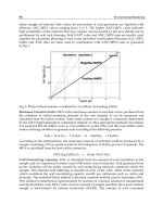
Third, the cell constant of the electrodes had to be estimated from the data. As shown in (2),
the cell constant can be estimated by dividing the known conductivity by the measured
conductance. The average estimated cell constant over all 7 measurements is 0.0867cm
-1
. The
measured conductivity of the water is plotted against the standard model of the
conductivity of seawater using a cell constant of 0.0867 below in Fig. 20.


Fig. 20. Correlation of known conductance of seawater (predicted) to actual data
(measured).
7. Conclusion
The Jag Ski provides a unique opportunity to collect hydrographic and environmental data
in shallow and remote areas typically inaccessible by traditional watercraft. Aside from its

PILS: Low-Cost Water-Level Monitoring

155
utility as a hydrographic data collection platform, it is small, inexpensive, and relatively
easy to maintain. Where a traditional vessel may require two or more people to launch,
operate, and recover, the PWC can easily be attended by one person if needed. With the
recent addition of the Portable SeaKeeper system, the Jag Ski’s capabilities have expanded
tremendously. The ability to map large spatial areas in a relatively small amount of time is
very helpful in coastal applications, mainly because it reduces the tidal bias of the collected
data. The Jag Ski’s speed and ease of deployment will also provide opportunities to perform
episodic surveys of coastal waters to determine the effects of storms or other events on the
near-surface water chemistry of Mobile Bay, Mississippi Sound, and nearby rivers.
The PILS unit combines low-cost components, including a novel low-cost salinity-measuring

circuit to provide a powerful and inexpensive environmental-monitoring capability. The
sensor package can readily be modified for other, similar missions. For example,
development is underway, using the microprocessor, clock, and salinity sensor, to develop a
system to control periodic GPS measurements and satellite transmissions to develop a low-
cost drifter to measure surface currents in the open ocean.
8. Acknowledgment
The authors wish to acknowledge the support of the following organizations in conducting
this work: The University of South Alabama College of Engineering, The University of
South Alabama Research Council, and The University of South Alabama University
Committee on Undergraduate Research (UCUR) Program. A portion of this material is
based upon work supported by the National Science Foundation under Grant No. OCE-
1058018.
9. References
Clifford, M. (2006). Water Level Monitoring, In : Freescale Semiconductor Application Note
AN1950, Rev. 4, Nov. 2006
Comeau, A.; Lewis, M., Cullen, J., Adams, R., Andrea, J., Feener, S., McLean, S., Johnson, K.,
Coletti, L., Jannasch, H., Fitzwater, S., Moore, C., & Barnard, A. (2007). Monitoring
the spring bloom in an ice covered fjord with the Land/Ocean Biogeochemical
Observatory (LOBO), Proceedings of OCEANS 2007
Dugan, J. P.; Vierra, K. C., Morris, W. D., Farruggia, G. J., Campion, D. C., & Miller, H. C.
(1999). Unique vehicles for bathymetric surveys in exposed coastal regions,
Proceedings of the Hydrographic Society of America Conference, April 27-29, 1999
Dugan, J. P.; Morris, W. D., Vierra, K. C., Piotrowski, C. C., Farruggia, G. J., & Campion, D.
C. (2001). Jetski-based nearshore bathymetric and current survey system. Journal of
Coastal Research, Vol. 17, No. 4, pp. 900-908
Freitag, L.; Johnson, M., & Preisig, J. (1998). Acoustic communications for UUVS. Sea
Technology, Vol. 39, No. 6, pp. 65–71
Frolov, S .; Baptista, A., & Wilkin, M. (2008). Optimizing fixed observational assets in a
coastal observatory. Continental Shelf Research, Vol. 28, No. 19, pp. 2644-2658
Frye, D. E.; Kemp, J., Paul, W., & Peters, D. (2001). Mooring developments for autonomous

ocean-sampling networks. IEEE Journal of Oceanic Engineering, Vol. 26, No. 4, pp.
477-486
Greenberg, A.; Clesceri, L., & Eaton, A. (1992). Standard Methods for the Examination of Water and
Wastewater 18th Edition, The American Public Health Association, Washington D.C.