793
23
Economics
The economics of treatment wetlands consists of two major
factors: capital costs and operating costs. The capital cost
components of free water surface (FWS) and subsurface
ow (SSF) wetlands are essentially the same, except for the
cost of the gravel required for SSF wetlands (Campbell and
Ogden, 1999; U.S. EPA, 2000a). However, SSF systems have
generally been implemented for smaller ows than FWS
systems. For instance, the system database compiled by the
Water Environment Research Foundation (WERF) has 214
FWS wetlands with a median design ow of 1,050 m
3
/d, 707
HSSF wetlands with a median design ow of 9.5 m
3
/d, and
566 VF wetlands with a median design ow of only 2.1 m
3
/d
(Wallace and Knight, 2006). System areas from the WERF
database show 330 FWS wetlands with a median area of 1.6
ha (16,000 m
2
), 710 horizontal subsurface ow (HSSF) wet-
lands with a median area of 140 m
2
, and 544 vertical ow
(VF) wetlands with a median area of 44 m
2

. Therefore, SSF
wetlands do not enjoy the economy of scale experienced by
FWS wetlands. There is now enough information to deter-
mine approximate capital cost functions that represent these
scale effects.
Because wetland systems are constructed using local
labor and local materials, it is not possible to offer precise
universal cost estimates that will apply to all treatment sys-
tems. Generally, the basic components of a wetland treatment
system—earthwork, gravel (in the case of SSF wetlands), lin-
ers, and plants—are produced in regional markets that are
distance sensitive. For instance, the installed cost per cubic
meter of gravel is highly dependent on the distance between
the source of supply (a local gravel pit) and the site of wet-
land construction. Labor costs are also highly variable. To
assess the feasibility of a wetland treatment system, local
cost gures should be used to compare the capital and oper-
ating costs of a wetland system against that of other treatment
technologies.
Within the United States, Construction Cost Indices
(CCI) are published by the Engineering News Record (ENR).
These cost indices track inationary changes within the con-
struction industry over time. The ENR CCI started at 100 in
the year 1913 and has increased to 7,856 in March 2007. Cost
indices are available as a national average, but are also pub-
lished for 20 major metropolitan areas in the United States.
For the purposes of this chapter, costs are based on the 2006
United States national average ENR CCI of 7,751. As a side
note, construction in high-cost metropolitan areas is almost
double that of low-cost metropolitan areas.

In general, capital costs of treatment wetlands are
comparable to alternative technologies for accomplishing
the same task. However, the costs of operating a treatment
wetland are typically much lower than for competing tech-
nologies. Mechanical devices are always more energy inten-
sive, and will always be more expensive to operate, than a
passive wetland system (Type A) (Brix, 1999). The basic
exchange is land for energy (Campbell and Ogden, 1999).
As a consequence, the lifecycle cost of a wetland project,
as represented by the present worth of capital and operating
expenses, is very often quite favorable compared to alterna-
tive treatment technologies.
Operating costs can be quite low, especially for Type A
passive systems. Energy costs are typically close to zero for
gravity-driven FWS wetlands, and are generally low for all
t
y
pes of treatment wetlands (see Table 1.1). Water quality
monitoring is often a principal part of O&M costs. However,
operation and maintenance (O&M) costs can become appre-
ciable if it is attempted to maintain specic vegetation types,
thus encountering “weeding” costs.
23.1 CAPITAL COSTS
Although it is not possible to offer universal cost guidelines,
every system shares a similar set of construction compo-
nents. Therefore, it is possible to estimate the cost of each
component within a regional market. The basic direct cost
components of a wetland treatment system include:
Land
Site investigation and system design

Earthwork
Liners
Media
Plants
Water control structures and piping
Site work (site preparation, fencing, access roads,
etc.)
Human use facilities
These costs include material, labor, overhead, and prot, and
represent the contractors installed cost. Additionally, there
are indirect costs associated with permitting, engineering,
nancing, mobilization, and construction management. In
general, these costs are all incurred prior to system start-up.
Detailed estimates are usually made after nal sizing and sit-
ing. More precise economic estimating is possible after nal
design drawings have been prepared.
REGIONAL VARIATION
Economics vary geographically because of differing unit
costs, and because of differences in the selection of materials
•
•
•
•
•
•
•
•
•
© 2009 by Taylor & Francis Group, LLC
794 Treatment Wetlands

and other design features. The cost of labor and materials
within a particular regional market plays a large role in the
cost of a wetland treatment system. Cost differentials are
even greater when comparing across worldwide geographic
locations and their accompanying economies. The effect
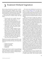
of regional market cost factors is illustrated in Figure 23.1,
which demonstrates treatment wetland capital cost distri-
butions for various locations. HSSF wetland systems in
Poland (Kowalik and Obarska-Pempkowiak, 1998) exhibit
lower capital costs than those in Nicaragua (Platzer et al.,
2002) or the Czech Republic (Vymazal, 1996). Severn Trent
tertiary systems in the United Kingdom (Green and Upton,
1994) are more expensive than those in the Czech Repub-
lic; HSSF systems in the United States have a distribution
of capital costs that spans the range from the inexpensive
Czech systems to those that are more expensive than the
U.K. systems.
Some of the regional differences have to do with design
sizing criteria. Different criteria are used in different coun-
tries, and also at different times in the same country. Others
have to do with structural specications. For instance, a num-
ber of U.K. systems are sited in basins lined with brick or
concrete, and some have stainless steel level and ow con-
trol elements. Clearly, such systems will have greater capital
costs than those sited in earthen basins with plastic piping
and simplied ow control elements.
There are also economies of scale, which will be
addressed in a subsequent section. However, it is useful to
rst examine the various components of capital costs in more
detail.

0.0
0.1
0.2
0.3
0.4
0.5
0.6
0.7
0.8
0.9
1.0
1 10 100 1,000 10,000
Cost ($1000 USD/ha)
Percentile
Poland
FWS USA
Central America
Czech
USA
Severn Trent
FIGURE 23.1 Capital costs distribution for treatment wetlands. All are HSSF systems except FWS (United States). Costs adjusted to 2006
using CCI  7,751 and the 2006 exchange rate. Data for Poland from Kowalik and Obarska-Pempkowiak (1998) In Constructed Wetlands
for Wastewater Treatment in Europe. Vymazal et al. (Eds.), Backhuys Publishers, Leiden, The Netherlands, pp. 217–225. Data for the Czech
Republic from Vymazal (1996) Ecological Engineering 7: 1–14. Data for Severn Trent from Green and Upton (1994) Water Environment
Research 66(3): 188–192. Data for Central America from Platzer et al. (2002) Investigations and Experiences with Subsurface Flow Con-
structed Wetlands in Nicaragua, Central America. Mbwette (Ed.). Proceedings of the 8th International Conference on Wetland Systems
for Water Pollution Control, 16–19 September 2002, Comprint International Limited: University of Dar Es Salaam, Tanzania, pp. 350 –365.
Data for the United States: Various.
DIRECT COSTS
Land

Land costs are highly site specic. Information on land avail-
ability and land costs is generally obtained with the assis-
tance of real estate professionals who are familiar with local
market conditions. Wetlands are more land intensive than
many other wastewater treatment processes. If land needs to
be purchased for the project, this can be a signicant cost
component. In the United States, treatment wetland land
purchase prices have ranged from $3,000/ha in remote loca-
tions with low population density and low agricultural utility
to over $100,000/ha in urbanizing agricultural landscapes.
Land acquisition in or near urban areas is sometimes viewed
as preservation of green space, and valued for ancillary
benets.
Land costs can be a signicant fraction of the total capi-
tal cost. For example, Wossink and Hunt (2003) identify
three categories of land cost for urban stormwater wetlands
in North Carolina: zero cost because the project is required
for community green space, $125,000/ha for vacant land that
may be used for residential development, and $550,000/ha
for land that may be used for commercial development.
As will be discussed, land costs occupy a special role in
the present worth analysis of a wetland system.
Site Evaluation
The design and construction of a wetland requires that
site characteristics be well understood—including soils,
© 2009 by Taylor & Francis Group, LLC
Economics 795
groundwater elevations, and site topography. These activi-
ties usually precede or accompany engineering design, but
are additional to that design.

Topographic Survey
The ground elevation of the site is a critical factor in design,
because it controls the cut-and-ll calculations that normally
dictate the elevations of berms and bottoms. Associated
with balancing of earth import and export is the issue of the
potential for gravity ow. Sometimes proper cell elevations
can eliminate the need for one or more pumps, and thus may
interact with cut-and-ll considerations. The topographic sur-
vey will inuence the direction of ow and the sequencing of
cells, and the need for long or short distribution and collec-
tion canals, which for large systems can inuence the project
cost. The potential need to level cell bottoms for purposes
of evening the hydraulic ow distribution can only be evalu-
ated with detailed site topography. The shallow water depths
in wetlands, especially large FWS systems, creates a need
for accurate as-built topography as an aid to understanding
water depth and movement. The costs for such surveys are
typically $50/ha–$500/ha, depending on scale and grid size
requirements. For instance, the topographic survey for the
Incline Village, Nevada, treatment wetland cost $370/ha for
the 175-ha wetland, adjusted to 2006. However, the survey
work for cell 4 of STA2 of the Everglades phosphorus control
project required only $45/ha.
Geotechnical Investigations
Many small-scale wetland projects are designed in conjunc-
tion with soil inltration systems. In these situations, it is
common to use shallow soil borings or backhoe pits to deter-
mine local soil characteristics. Costs for these initial site
investigations vary with the size of the project. In the U.S.,
the cost for a site investigation can range from a few hundred

dollars (for a single-home system) up to several thousand dol-
lars (for a system serving a small community).
Larger-scale projects, including those that discharge to
surface waters, also require soil investigations. Even though
such large projects rarely require liners, there is a need to
assess the potential for seepage from the project, and hence
the need for seepage collection canals. It is critical to deter-
mine if site soils are adequate for the berms and levees, and
if so how much compaction may be required, and how much
allowance for subsidence.
Soils that may be used for rooting media in FWS systems,
as well as the gravel substrate for SSF systems, may need to
be assessed for contaminants of concern, including nutrients.
A modest amount of chemical testing may be required to
identify any potential problems, or to form the basis for fore-
casting the sorption life expectancy for contaminants.
Hydrogeological Investigations
The location of the groundwater table and direction of
groundwater movement can be a critical factor in wetland
design. For small community and on-site systems involving
soil inltration, the depth to groundwater is an important
consideration. For “normal” inltration beds (septic elds),
there is a required minimum unsaturated depth that is likely
to carry over to the wetland/inltration situation.
For a wetland with a liner, it is also necessary to know the
depth to groundwater, because rising, shallow water tables
can lift a synthetic wetland liner, displacing air from the soil
environment. This has the potential to create large under-
liner bubbles that push the liner up out of the water; these are
commonly called “whale backs.” The solution to such poten-

tial difculties is the construction of an under-drain system
beneath the wetland liner that vents air and controls the level
of the water table. The need for this feature, and its associ-
ated cost, will be determined through site-specic hydrogeo-
logical investigations.
In some cases, there may be a concern for regional use
of the groundwater as a potable water supply. The treatment
wetland might be viewed as a possible source of contamina-
tion if partially treated water entered into the unprotected
drinking water aquifer, and moved to the wells that withdraw
potable water. This would usually occasion the need for a
hydrogeological study to ascertain the depths and directions
of regional groundwater ow, and the consequences of even
small leaks from the treatment wetland to the water quality of
the aquifer. This was the case at the Columbia, Missouri, proj-
ect. The hydrogeological study included calibration and mod-
eling to address this issue, at a cost of $750/ha for the 36-ha
wetland, adjusted to 2006 (Brunner et al., 1992).
Ea
r
thwork
The construction of a wetland treatment system requires
excavation and grading of the site to produce level basins that
are enclosed by earthen berms. For small systems (generally
less than 0.05 ha) backhoes or similar types of excavation
equipment are commonly used. Larger basins are generally
constructed using bulldozers or construction scrapers. Area-
specic earthwork costs are the product of two components.
The rst component is the cost to move earth, which is a
volumetric (per cubic meter) cost. This cost component is

a function of equipment costs, labor costs, and the source
of earth supply (on-site or imported). The second compo-
nent is the amount of earth that must be moved to grade the
site. This areal requirement (m
3
of earth per m
2
of wetland
area) is a function of the project site conditions. Earthwork
costs are lowest on at sites that require minimal grading
and have suitable soils on-site (low areal grading require-
ment and volumetric cost). Sloping a site requires terracing,
which increases earthwork costs (due to the large areal grad-
ing requirement). If the ll needs to be imported, earthwork
costs will increase (due to the high volumetric cost). Earth-
work construction techniques are essentially the same for
FWS and HSSF wetlands, and hence volumetric earthwork
costs for the two types should be comparable for similar-
sized wetlands.
© 2009 by Taylor & Francis Group, LLC
796 Treatment Wetlands
Clearing and Grubbing
If the undeveloped site has undesirable vegetation, build-
ings, or other existing features that are incompatible with
the wetland, these will need to be removed as part of the
earthwork process. Brush and trees were removed from the
sites at Ouray, Colorado; Sorrento, Louisiana; and West Jack-
son County, Mississippi, at an average cost of $9,800/ha. On
larger projects, roads and ditches may require degrading, and
buildings may require removal.

FWS Wetlands
In a study of two municipal FWS wetland systems (West
Jackson County, Mississippi and Gustine, California) the
U.S. Environmental Protection Agency (EPA) estimated a
volumetric cost of $10.80/m
3
when adjusted to 2006 USD
(U.S. EPA, 2000a). The 20.2-ha wetland system in West
Jackson County, Mississippi, had an areal grading require-
ment of only 0.26 m
3
/m
2
, and the 9.7-ha system in Gustine,
California, had an areal grading requirement of 0.35 m
3
/m
2
.
Larger treatment wetlands require far less earthmoving
on a per-hectare basis than do small systems. For instance,
Cell 4 of STA2 of the Everglades phosphorus control proj-
ect required only 0.056 m
3
/m
2
of earthmoving based on the
816-ha wetland footprint. However, the construction of such
a large system does not involve scraping a thin layer from the
entire footprint. Rather, the inlet spreader canal, outlet col-

lection canal, and seepage return canal are the source of the
ll material for the containment levees.
Even large wetlands may require signicant earthmov-
ing if built on sloping terrain. For example, the Inman Road
treatment wetland in Clayton County, Georgia, has 22 wetted
hectares in a terraced arrangement of 22 cells. The site pre-
sented slopes of 2–25%, and about 30 m of vertical variation
(Inman et al., 2001, 2003). Construction required moving
420,000 m
3
of earth, or 1.9 m
3
/m
2
.
Regional factors and site conditions can alter the cost of
earthmoving. Cell 4 of STA2 of the Everglades phosphorus
control project moved 460,000 m
3
of material, in a nearly
balanced cut and ll. The breakdown of per cubic meter costs
was: $2.61 to blast rock, $2.13 to excavate, and $2.09 to build
levees, for a total of $7.96/m
3
(adjusted to 2006 USD).
HSSF Wetlands
Earthwork costs for some HSSF wetland systems in the
Minnesota–Wisconsin regional market are summarized in
Ta
ble 23.1. Data from these seven HSSF wetland systems

clearly show the impact of local site conditions on earthwork
costs. Areal grading requirements varied from 0.21 m
3
/m
2
to
1.73 m
3
/m
2
, with a median value of 1.03 m
3
/m
2
.
Volumetric earthwork costs for the systems in Table 23.1
varied between $2.17/m
3
and $18.15/m
3
, with a median value
of $7.56/m
3
(cost adjusted to 2006 USD, ENR CCI  7751).
Combining areal grading requirements with volumetric
earthwork costs resulted in areal earthwork costs ranging
between $1.68/m
2
and $13.97/m
2

, with a median value of
$5.06/m
2
(adjusted to 2006 USD).
Liners
The decision to install a liner in a wetland system, and which
type of liner to use, depends on the project goals, regulatory
requirements, and feasibility. Some wetlands are unlined,
either because the in situ native soils are deemed to have suf-
cient sealing properties, or because groundwater recharge is
a function of the system. Very large FWS wetlands cannot be
plastic lined because it is not feasible for systems of more than
a few hectares, but clay lining has been implemented on sys-
tems up to 40 ha, such as Columbia, Missouri. If the wetland
must be lined, there are a variety of liner materials available.
The two most common liner materials used are 0.76-mm
polyvinyl chloride (PVC) and 1.0-mm high-density poly-
ethylene (HDPE). PVC liners are generally factory seamed,
one-piece liners used on small projects less than 0.1 ha
in size. HDPE liners generally come in rolls and are eld
seamed for larger projects.
The total installed cost of the liner includes not only the
material cost but also the labor cost associated with eld
seaming, seam testing, material inspection, and leak test-
ing. If local soil conditions include sharp or angular rocks,
TABLE 23.1
Earthmoving Costs for HSSF Wetlands in Minnesota
System Name
Design
Flow (m

3
/d)
Wetland
Area (m
2
)
Earthwork
Volume (m
3
)
Cost
Volumetric
($/m
3
)
Grading Req.
(m
3
earth per
m
2
wetland)
Cost (Areal)
($/m
2
)
St. George, Minnesota 25 595 631 8.54 1.06 9.06
Darfur, Minnesota 38 1,301 383 5.70 0.29 1.68
Northern Tier High Adventure Base, Minnesota 34 297 306 13.56 1.03 13.97
Lakes of Fairhaven, Minnesota 59 1,828 383 7.56 0.21 1.58

Delft, Minnesota 22 664 306 18.15 0.46 8.36
St. Croix Chippewa, Wisconsin 251 6,141 6,885 4.51 1.12 5.06
Prinsburg, Minnesota 206 4,094 7,069 2.17 1.73 3.75
Median Values 7.56 1.03 5.06
© 2009 by Taylor & Francis Group, LLC
Economics 797
a layer of sand or other granular material may have to be
placed before the liner can be installed. If the gravel used
to line the bed has sharp or angular edges, it may be neces-
sary to cover the interior of the liner with a protective layer
of geotextile fabric, since sharp rock can puncture a liner.
Table 23.2 shows approximate installed costs of a variety of
liner materials.
Liner costs for the FWS wetland system at Ouray, Colo-
rado, were $6.97/m
2
, and $13.23/m
2
for the HSSF wetland sys-
tem at Ten Stones, Vermont (both adjusted to 2006 USD) (U.S.
EPA, 2000a). Liner and geotextile fabric costs for 12 HSSF
wetlands in the Minnesota–Wisconsin regional market are
summarized in Table 23.3. Data from these wetland systems
indicate that installed liner costs (adjusted to 2006 USD; ENR
CCI  7751) ranged from $3.74/m
2
to $19.71/m
2
, with a median
cost of $8.66/m

2
. The use of a geotextile fabric will increase
the installed liner cost. The data in Table 23.3 indicate that the
installed cost will increase by approximately $3.00/m
2
when a
geotextile fabric is used.
If soil at the site contains rocks or other debris that could
damage the liner during installation, a layer of sand or similar
granular material is often placed prior to installing the liner.
For example, 8 cm of sand was placed prior to installing the
liner in three Minnesota HSSF wetlands. The installed cost
for sand bedding ranged from $1.38/m
2
to $3.08/m
2
, with a
median cost of $2.24/m
2
(2006 USD; ENR CCI  7751).
Media and Mulch
The major cost variation between FWS and SSF wetlands
results from differences in the rooting media. FWS systems
typically use 30–40 cm of soil, which may be entirely avail-
able on the site, whereas SSF wetlands use 50–80 cm of
gravel or other similar media, which must usually be pur-
chased and transported to the site.
Soils for FWS Systems
If in situ native soils are suitable, they are typically used as
the rooting substrate for emergent wetland plants in FWS

systems. If in situ native soils are unsuitable for use as root-
ing media, soil may be imported and mixed with existing
soil to create conditions adequate for rooting wetland plants.
For these reasons, the cost of the rooting medium is usu-
ally reected in the volumetric earthwork costs. However,
it is sometimes advantageous to add organic material to the
rooting soil for a FWS system, to provide sorption capac-
it
y immediately upon start-up (Figure 23.2). Such a blending
TABLE 23.2
Approximate Cost of Installed Liners (2006 USD)
Material Thickness
Installed Cost
($/m
2
)
Bentonite 10 kg/m
2
7.96
Native clay
a
30 cm 7.50
Clay geotextile sandwich NS 4.84
Polyvinyl chloride 0.76 mm 4.09
High-density polyethylene 1.02 mm 4.73
Polypropylene 1.02 mm 5.92
Reinforced polypropylene 1.14 mm 6.89
Hypalon 0.76 mm 6.89
Hypalon 1.52 mm 8.07
XR-5 NS 11.19

a
Assumes $25/m
3
delivered, placed, and compacted.
Source: Data from U.S. EPA (2000a) Constructed wetlands treatment of
municipal wastewaters. EPA 625/R-99/010, U.S. EPA Ofce of Research
and Development: Washington D.C.; and Interstate Technology and Regula-
tory Council (2003) Technical and Regulatory Guidance Document for Con-
structed Treatment Wetlands. />TABLE 23.3
Liner and Geotextile Costs for Example HSSF Wetlands
System Name
Design
Flow (m
3
/d)
Wetland
Area (m
2
)
Liner
($/m
2
)
Geotextile
($/m
2
)
St. George, Minnesota 25 595 8.04 —
Darfur, Minnesota 38 1,301 7.36 3.35
Northern Tier High Adventure Base, Minnesota 34 297 8.93 1.84

Opole, Minnesota 35 725 6.57 3.94
Tamarack, Minnesota 26 418 19.71 3.29
Lakes of Fairhaven, Minnesota 59 1,828 6.84 3.02
Delft, Minnesota 22 664 13.70 12.45
Cedar Mills, Minnesota 35 1,073 9.95 1.76
St. Croix Chippewa, Wisconsin 251 6,141 3.74 0.82
Prinsburg, Minnesota 206 4,094 10.19 —
Mulberry Meadows, Minnesota 72 1,580 8.39 2.47
Cambridge-Isanti School District, Minnesota 39 1,196 9.07 3.13
Median Value 8.66 3.08
Note: Geotextile is a nonwoven, needle-punched polypropylene material (230 g/m
2
fabric weight) used as a protective
layer on top of the liner.
© 2009 by Taylor & Francis Group, LLC
798 Treatment Wetlands
operation may involve approximately 10 cm of amendment
material, thus adding 0.1 m
3
/m
2
of earthmoving to the proj-
ect, plus the cost of the composting material. Municipal yard
waste compost has been successfully used at Isanti-Chisago,
Minnesota, and at Saginaw, Michigan, treatment wetlands.
The use of purchased topsoil, either entirely or as an amend-
ment, is a very expensive option, because high-quality (hor-
ticultural) topsoil typically sells for up to $25/m
3
.

Media for SSF Wetlands
A number of innovative types of media have been used in
SSF treatment wetlands. Examples include recycled glass
fragments, such at Millersylvania State Park, Washington,
blast furnace slag (Mann and Bavor, 1993; Drizo et al., 1999),
and lightweight expanded clay aggregates (LECA) (Zhu et
al., 1997; Jenssen and Krogstad, 2003). The cost of LECA is
quite high; for instance, Scholz et al. (2001) report $204/m
3
(2006 costs), but it is available in large units (Figure 23.3).
The wide variety of SSF wetland media leads to wide varia-
tions in costs, but gravel is perhaps the most common mate-
ri
al used in Europe and North America (Figure 23.4).
In a HSSF wetland, the rooting medium comprises the
material used in the main wetland bed (typically gravel) and
the coarser material used in the inlet and outlet zones (typi-
cally coarse rock). Costs for these materials are a function of
regional market conditions as well as the distance between
the source of supply and the project site. For instance, the 4.0-
ha VF wetland at Connell, Washington, utilized 36,000 m
3
of
2.6-mm coarse sand that was available immediately adjacent
to the bed, thus incurring only a cut-and-ll cost (Burgoon
et al., 1999). That situation is extremely rare, and most often
media will be mined, screened, washed, and transported to
the wetland site at considerable cost.
Media costs for 12 selected HSSF wetlands in the Minne-
so

t a – W i s c o n s i n r e g i o n a l m a r k e t a r e s u m m a r i z e d i n Ta b l e 2 3 . 4 .
This region was glaciated and typically has ample sources of
gravel within a reasonable distance of a project. Data indicate
that installed gravel media costs (used in the main portion
of the bed) range between $15.95/m
3
and $70.26/m
3
, with a
median cost of $41.87/m
3
(adjusted to 2006 USD). The gravel
used in these systems was 9–25 mm in size. Within the Min-
nesota–Wisconsin regional market, distances between the
source of supply (local gravel pit) and the project site were
the primary factor in determining unit costs. As the depth of
the bed media is established during the design process, cal-
culation of areal costs is relatively straightforward. All of the
HS
SF systems in Table 23.4 were designed with a bed depth
of 0.45 m, resulting in a median areal cost of $18.84/m
2
.
Media costs presented in Table 23.4 are higher than those
presented in the literature for other HSSF systems. For three
HSSF wetlands (Mesquite, Nevada; Carville, Louisiana; and
Ten Stones, Vermont), U.S. EPA (2000a) reported bed media
costs of $14.33, $23.58, and $14.74/m
2
, respectively (2006

USD). These were deeper beds (0.8, 0.75, and 0.75 m, respec-
tively), and the volumetric cost of the media was less.
FIGURE 23.2 Organic materials may be added to the rooting soils to promote early sorption potential. At the Hillsdale, Michigan, site,
soils were borrowed from an adjacent oodplain, creating a pond and island complex in the borrow site.
FIGURE 23.3 Light expanded clay aggregate (LECA) can be pur-
chased in large units in Europe.
© 2009 by Taylor & Francis Group, LLC
Economics 799
Mulch
In cold-climate regions, it may be necessary to insulate a
HSSF system. This may be done with straw, or cover blankets
for small systems. Mulch may be used as an insulating layer
for cold-climate wetlands, and is a common design feature
of HSSF wetlands in Canada and the northern regions of the
United States (Figure 23.5). All of the wetlands in Table 23.4
were insulated with 0.09 m of reed-sedge peat. Installed costs
for this peat material (2006 USD) ranged between $23.94/m
3
and $82.98/m
3
, with a median cost of $49.89/m
3
. This con-
verts to an areal cost of $4.49/m
2
.
Coarse Stone
The berm slopes of FWS wetlands may be armored against
burrowing animals and wave erosion by the use of rip rap.
Co

arse rock is a common choice (see Figure 18.19), but con-
crete matting has also been used (see Figure 18.23).
HSSF wetlands commonly use a coarser material (drain
ro
ck) in the inlet and outlet portions of the bed (Figure 23.6).
In the United Kingdom, the stone inlet and outlet zones are
typically 0.5 m wide, at full bed depth, and packed with 50–
200 mm stone (Cooper et al., 1996). Drain rock used in the
12 HSSF wetlands summarized in Table 23.4 was 20–75 mm
in size. Installed drain rock costs ranged from $25.53/m
3
to
$74.41/m
3
, with a median cost of $47.59/m
3
(adjusted to 2005
USD). U.S. EPA (2000a) reports that costs for outlet materials
were $10.39/m
3
(50-mm stone) and $24.24/m
3
(100-mm stone)
for the HSSF wetland at Ten Stones, Vermont (2006 USD).
Plants
The plant component of capital cost varies according to the
method chosen for vegetation establishment. It is presup-
posed that the media is in place, either the soil layer in a
FWS system or the gravel in an SSF system. The FWS
FIGURE 23.4 Gravel media being placed at the Grand Lake, Minnesota, HSSF wetland.

TABLE 23.4
Media Costs for Selected HSSF Wetlands
System Name
Design
Flow (m
3
/d)
Wetland
Area (m
2
)
Gravel
($/m
3
)
Mulch
($/m
3
)
Coarse
Stone ($/m
3
)
St. George, Minnesota 25 595 31.32 82.98 48.00
Darfur, Minnesota 38 1,301 45.56 81.36 47.18
Northern Tier High Adventure Base, Minnesota 34 297 70.26 76.64 74.41
Opole, Minnesota 35 725 15.95 49.47 31.11
Tamarack, Minnesota 26 418 23.94 23.94 25.53
Lakes of Fairhaven, Minnesota 59 1,828 33.27 45.36 52.92
Delft, Minnesota 22 664 42.33 37.80 36.30

Cedar Mills, Minnesota 35 1,073 39.83 64.02 52.65
St. Croix Chippewa, Wisconsin 251 6,141 41.40 32.44 30.31
Prinsburg, Minnesota 206 4,094 45.53 55.48 52.65
Mulberry Meadows, Minnesota 72 1,580 51.65 46.22 51.66
Cambridge-Isanti School District, Minnesota 39 1,196 46.22 50.30 44.87
Median Value 41.87 49.89 47.59
© 2009 by Taylor & Francis Group, LLC
800 Treatment Wetlands
wetland offers the largest number of options, including natu-
ral recruitment, seeding, and planting.
Natural Recruitment
This option is the least costly but the least controllable,
and usually of the longest duration. It is not free from cost,
because moist soil conditions must be maintained, which in
turn requires water management on the wetland. Virtually
all of the Florida stormwater treatment wetlands (STAs) were
established in this way. A newer strategy for these STAs is
the use of a seeded sacricial rice cover crop (Oryza sativa),
which assists in soil stabilization and initial nutrient immobi-
lization. This cover crop lasts only one growing season, does
not renew itself, and gives way to other wetland vegetation.
Seeding
Seeding is the next least expensive method of vegetation
establishment. The techniques range from scattering in the
wi
nd (Figure 23.7), to back-pack broadcasting, to the use of
seed drills. The seed is then pressed into the soils using a
roller or cultipacker, or by light raking. The use of foot travel
has also been used effectively, at the Isanti-Chisago site in
Minnesota (Loer et al., 1999). Volunteer labor has been used

successfully at Brighton, Ontario, and Roblin, Manitoba,
where grades 9 and 10 science students participated in seed-
ing (PFRA, 2002). Hydroseeding has been used successfully
(U.S. EPA, 2000a) but requires the addition of detergent to
loosen the seed covering. In the Great Lakes region of the
United States, the optimum seeding time is autumn through
late spring.
Seeds for wetland plants may be harvested from local
sources as part of the project work, particularly for Typha,
which produces large seed heads with extremely numerous
seeds, and which are easily picked in autumn. Seeds are also
available from wetland nurseries in the United States, for over
a hundred wetland species. The cost is considerable, ranging
from $125 to $1,500 per kilogram of live seeds for common
wetland plants in the northern United States (Table 23.5). The
seeding rate is typically on the order of 2–4 kg of live seed
per hectare. The purchased price of the seed is consequently
in the range of $400–$3,000 per hectare, with a median of
about $1,200 per hectare. The cost of installation includes the
seeding itself (minor) and the fostering of germination and
growth, via soil moisture/water management (major). Dry
seeding has been estimated at ten man-hours per hectare,
and hydroseeding at $145/ha (U.S. Army Corps of Engineers,
2000). Such required activities are usually inexpensive, and
are less than the cost of the seed itself.
FIGURE 23.5 Peat mulch in place at the Grand Lake, Minnesota, wetland.
FIGURE 23.6 Inlet coa rse rock zone at t he Fish and Royer, I ndia na ,
HSSF wetland.
© 2009 by Taylor & Francis Group, LLC
Economics 801

Planting
The choice to plant originates with the desire to propagate
a selected suite of plant species in a short period of time.
Planting costs are a function of several different factors.
These include the form of plant material (plugs or rootstock),
FIGURE 23.7 Seeding of the Brighton, Ontario, wetland (a) and the resulting growth (b). (Photos courtesy J. Pries.)
(a)
(b)
TABLE 23.5
Examples of Prices for Plants and Seeds (2007 USD)
Seed Bare Root Plugs
($/kg) ($/ha) ($/Plant) ($/ha) ($/Plant) ($/ha)
Individual Species
Phragmites australis Common reed — — 0.65 6,500 0.95 9,500
Phalaris arundinacea Reed canarygrass — — 0.55 5,500 — —
Typha latifolia Broad leaf cattail 127 381 0.80 8,000 0.98 9,750
Typha angustifolia Narrow leaf cattail 127 381 0.80 8,000 1.08 10,750
Scirpus validus Great bulrush 485 1,454 0.65 6,500 0.80 8,000
Scirpus acutus Hard-stemmed bulrush 717 2,152 0.85 8,500 0.88 8,750
Scirpus atrovirens Dark green rush 329 986 0.85 8,500 0.88 8,750
Scirpus pungens Common three-square 1,072 3,217 0.65 6,500 0.90 9,000
Scirpus cyperinus Woolgrass 326 978 0.60 6,000 0.83 8,250
Iris virginica Blue-ag iris 357 1,070 0.85 8,500 1.15 11,500
Leersia oryzoides Rice cutgrass 419 1,258 0.40 4,000 0.80 8,000
Juncus effusus Common rush 599 1,797 0.55 5,500 0.88 8,750
Sagittaria latifolia Common arrowhead 374 1,121 0.55 5,500 1.25 12,500
Pontederia cordata Pickerel weed 317 952 2.00 20,000 3.13 31,250
Sparganium eurycarpum Common bur reed 431 1,293 0.55 5,500 1.28 12,750
E
mergent Wetland Mix

(20 species plus cover crop) — 3,088 — — — —
Stormwater Wetland Mix
(18 species plus cover crop) — 1,914 — — — —
Rush/Bulrush Mix
(5 species) — 556 — — — —
Median 1,189 0.65 6,500 0.93 9,250
Note: The
planting rate is assumed to be 10,000/ha, and the seeding rate is assumed to be 3.0 kg/ha. The cover crop is 25 kg/ha common oats (Avena sativa)
and 8 kg/ha of annual rye (Lolium multiorum).
Source: Data based on averages from J.F. New, Walkerton, Indiana ( and Southern Tier Consulting, West Clarksville, New York
( />the source of material (locally harvested, on-site nursery,
or commercial nursery), the method of planting (manual or
mechanical, volunteer or, contractor labor), and the overall
planting density (number of plants per square meter). Because
© 2009 by Taylor & Francis Group, LLC
802 Treatment Wetlands
of these variables, planting costs vary widely among wetland
projects. In projects that employ hand planting, plant mate-
rial costs may be a small fraction of the installed cost.
Commercial nurseries sell a wide range of wetland plants
as potted “plugs” or bare root stock (Table 23.5). The median
(2007) cost of bare root propagules was $0.65 (n  14), and
for plugs, $0.93 (n  13). Transportation costs must be added
to these, leading to a delivered cost of about $1.20 per plant.
It is sometimes possible to obtain plants from existing stands,
such as cattails from roadside ditches. Extraction requires
mechanical digging, typically with a backhoe, to a depth of
about 30 cm, so as to gather the majority of the root mass. The
plants are then separated from the mass by hand, with each
propagule containing at least one healthy shoot and at least 20

cm of associated rhizome. The shoot is topped to a height of
30–40 cm, to reduce the amount of foliage that the transplant
must maintain after the trauma of transplanting. On-site nurs-
eries may also be established prior to wetland construction, for
the purpose of supplying plant materials. However, the plant-
ing contractor may prefer to avoid the effort needed to extract
and prepare the plants, and opt for the use of purchased plants,
as was the case at Columbia, Missouri (Brunner and Kadlec,
1993). Established treatment wetlands may serve as sources of
plant materials for new systems. For example, the plants for
the Connell, Washington, system (Kadlec et al., 1997) were
extracted from the Arcata, California, project, and success-
fully established in the new wetland. Marsh establishment
on the Texas coast required 11.3–29.3 man-hours per 1,000
plants to hand-dig, separate, and transplant various propagule
types of 11 marsh species (Dodd and Webb [1975], as refer-
enced by U.S. Army Corps of Engineers [2000]).
The total cost of plants depends on planting density,
which ranges over about 0.25–4.0 plants per square meter
(spacing of 0.5–2.0 m). If the plants are on 1-m centers, there
a
r
e 10,000 per hectare. This value is used in Table 23.5 to
establish the per-hectare cost of nursery-purchased plant
plugs, which ranges from $8,000 to $31,000, with a median
of $9,250/ha.
The cost of putting the plants into the ground can be
extremely variable. In some instances, innovation has been
employed to quickly and efciently plant a wetland with
mechanical equipment (Figure 23.8). However, most small

wetlands are planted by hand, with rates of up to 150 plants per
person per hour for experienced planting crews. Allowing for
lesser efciency of 50 plants per person per hour, thus requir-
ing 200 man-hours per hectare at 10,000 plants per hectare.
This matches estimates provided by the U.S. ACE publication
(U.S. Army Corps of Engineers, 2000). For labor at $20/h,
insertion costs would be about $2,000/ha at 10,000 plants per
hectare, or $0.40 per plant. When combined with the per-plant
purchase price, the cost would be $1.60 per plant installed.
U.S. EPA (2000a) suggests a planting cost for FWS wet-
lands of $0.83 per plant installed (adjusted to 2006 USD).
This may be a reasonable estimate for locally harvested
plants, but is probably too low for nursery-purchased plants.
Table 23.6 summarizes planting costs for HSSF wet-
land systems in the Minnesota–Wisconsin, U.S. regional
market. All of these systems were hand-planted with root-
stock (primarily Scirpus atrovirens, Scirpus uviatilis, and
Scirpus cyperinus) purchased from commercial wetland
plant nurseries in Wisconsin. All 12 systems were planted
at a density of 2.7 plants/per square meter. This represents
an aggressive planting approach that uses well-established
rootstock and is designed to achieve complete plant cover-
age in about two growing seasons (which is approximately
18 weeks per year in this climatic region). The median of
$4.58 per plant installed, in Table 23.6, is much higher
than the estimate mentioned previously. The difference may
be attributable not only to labor costs and other regional
market factors but also to the unfamiliarity of the contrac-
tors with planting as a construction activity. On an areal
basis, Table 23.6 shows a median of $12.32/m

2
. In another
adjacent climatic region, for the Minoa, New York, HSSF
wetland, planting costs were $9.45/m
2
.
For small to medium size wetlands (less than 10 ha),
planting costs are less than 10% of the total capital cost. This
FIGURE 23.8 Homemade planter used for the Hillsdale, Michigan, treatment wetland (a). The 1.4 ha of basins were quickly planted (b).
See Figure 19.6 for a view of the wetland one year later.
(a)
(b)
© 2009 by Taylor & Francis Group, LLC
Economics 803
fraction applies to all regions, such as Spain (Nogueira et al.,
2006). For very large FWS wetlands, planting is too expen-
sive, and natural recruitment is relied on.
Structures
Hydraulic control of wetlands is generally provided through
distribution piping and water level control structures. Inlet
distribution, outlet collection, and water level control are
required in all systems.
Many FWS systems operated with parallel paths, thus a
splitter structure is needed to apportion the ows among ow
paths. Depending on the size of the system and the complex-
ity of the structure, costs will vary, but may be about $5,000–
$10,000 for a 1-ha wetland (Wallace and Knight, 2006). In
FWS wetlands, inlet distribution is normally accomplished
using an inlet deep zone across the width of the wetland, also
called an inlet spreader canal. The cost for this is part of the

cut and ll for the overall project. These deep zones may be
lled with coarse rock to discourage rodents, thus incurring
the cost of the rock.
Sometimes a perforated pipe is placed at the bottom of the
deep zone, to aid in uniform introduction of the water. The
cost of 10-cm diameter perforated PVC is roughly $20/m.
In warm climates, distribution piping may be above ground
an
d above water (see Figure 18.23). Gated aluminum irriga-
tion piping costs on the order of $30/m for 30 cm diameter,
with lesser costs for smaller diameters. The 30-cm size can
convey up to 15,000 m
3
/d without excessive headloss, and
smaller diameters may be used for smaller ow rates.
Small HSSF wetlands may receive nearly raw waste-
water, which will necessitate some form of inlet trash screen-
ing. In the United Kingdom, this may be a Copasac™ cham-
ber with a lter bag; in other countries, a cleanable bar
screen is used. If the water is delivered from a septic tank,
or other settlement chamber, then this screening device may
be unnecessary.
In small- to mid-sized HSSF wetlands, ow is generally
distributed across the width of the bed in the inlet zone using
perforated pipes or inltration chambers. Perforated PVC
pipe (100-mm diameter) is commonly used as a low-cost dis-
tribution method for small systems. The drawback of using
perforated pipe is that the inuent organic loading is concen-
t
r

ated at the perforations. Inltration chambers (Figure 23.9)
have a louvered sidewall which provides a greater number
TABLE 23.6
Planting Costs for Selected HSSF Wetlands
a
System Name Design Flow
(m
3
/d)
Wetland Area
(m
2
)
Plants
($/plant)
Installed Cost
($/m
2
)
St. George, Minnesota 25 595 4.55 12.24
Darfur, Minnesota 38 1,301 4.36 11.73
Northern Tier High Adventure Base, Minnesota 34 297 6.11 16.44
Opole, Minnesota 35 725 12.22 32.87
Tamarack, Minnesota 26 418 8.54 22.97
Lakes of Fairhaven, Minnesota 59 1,828 2.89 7.77
Delft, Minnesota 22 664 4.63 12.45
Cedar Mills, Minnesota 35 1,073 4.61 12.40
St. Croix Chippewa, Wisconsin 251 6,141 2.72 7.32
Prinsburg, Minnesota 206 4,094 4.71 12.67
Mulberry Meadows, Minnesota 72 1,580 3.91 10.52

Cambridge-Isanti School District, Minnesota 39 1,196 3.39 9.12
Median Value 4.58 12.32
a
Costs in 2006 USD.
FIGURE 23.9 Placement of inlet distribution chamber at Lake
Elmo, Minnesota. (From Wallace and Knight (2006) Small-scale
constructed wetland treatment systems: Feasibility, design cri-
teria, and O&M requirements. Final Report, Project 01-CTS-5,
Water Environment Research Foundation (WERF): Alexandria,
Virginia. Reprinted with permission.)
© 2009 by Taylor & Francis Group, LLC
804 Treatment Wetlands
of openings and a larger cross-sectional area, both of which
are desirable for evenly distributing the inuent organic load.
Generally, the same device (perforated pipe or inltration
chamber) is used at the outlet end of the bed for efuent col-
lection. Installed costs for perforated pipe and inltration
chamber approaches in the northern United States are about
$20/m and $40/m, respectively (Wallace and Knight, 2006).
The water level within a wetland cell is regulated by a
downstream water level control structure. A typical outlet
structure for small FWS wetlands is shown in Figure 18.27,
and an outlet for a moderately large system in Figure 18.28.
The costs for typical low-ow level control structures are
given in Figure 23.10. A simple exible pipe outlet level con-
trol structure for a HSSF wetland is shown in Figure 23.11.
Some small systems use premanufactured “pond valves” that
utilize stacking plates (with a 100 mm inlet and outlet pipe) to
set the water level. Costs for this approach are below $1,000
for ows under 500 m

3
/d (Wallace and Knight, 2006). Larger
projects may use precast or cast-in-place concrete structures
with a weir device (stop log, xed plate, or adjustable weir
gate). The ability to adjust the water level is an important
control element, and providing operational control over the
water depth in the wetland is well worth the incremental cost
over xed-level structures.
Large inlet and outlet structures for FWS systems can
be fairly complicated, with many cost components (see Fig-
ure 18.22). These may involve remote sensing of water lev-
els, sent to an operations center by telemetry, and remote
control of opening and closing. Therefore, there is a need
for electrical power, and the associated control equipment.
The structure requires appropriate bedding, which usually
means imported gravel. The cost breakdown for an example
is given in Table 23.7. Despite the apparent complexity and
cost, such structures are more economical when measured in
terms of cost per unit ow rate. The structure of Table 23.7
cost approximately $0.42 per m
3
/d, whereas the AgriDrain™
units cost about $0.71 per m
3
/d.
0
500
1,000
1,500
2,000

2,500
3,000
0 500 1,000 1,500 2,000 2,500 3,000 3,500 4,000
Capacity (m
3
/d)
List Price ($)
1.83 m
3.05 m
FIGURE 23.10 Example pricing of simple in-line stoplog structures. The height of these contained units is variable; data are shown for
1.83 and 3.05 total structure height. The capacity is for a height over the weir of 25 cm. See Figure 18.26. (Data from Agri Drain Corpora-
tion, Adair, Iowa. Date: March 30, 2007, CCI  7,856. />FIGURE 23.11 Outlet level control structure at Pribraz, Czech
Republic. Flexible pipes may be raised or lowered to adjust water
level. There are two cells controlled by this device.
TABLE 23.7
Capital Cost of One Inlet Structure for STA2 Cell 4
Item Description Cost ($)
Piping 40 m of 1.68-m diameter @ $983/m 39,323
Structure Slide gate 29,595
Excavate, bed, install 917 m
3
gravel 9,095
Sensors — 21,244
Telemetry — 9,560
Stilling wells — 26,644
Electrical control — 36,115
Total 171,577
Note: Adjusted
to
2006 USD, CCI  7,751. There are six such structures

for the 816-ha wetland.
Source: Data from Brown and Caldwell (2005) Basis of design report,
Stormwater Treatment Area 2 Cell 4 Expansion Project. Report to South
Florida Water Management District. , West Palm
Beach, Florida.
© 2009 by Taylor & Francis Group, LLC
Economics 805
Site Work
These site work costs generally include construction ele-
ments such as construction of access roads to the project
site, fencing (if required), installation of electrical power
to the project site, erosion control, seeding (outside wetland
areas), and surface restoration. As the nature and extent of
these site work requirements change from project to project,
these costs will also vary. Fencing is a common require-
ment, and three-meter cyclone fencing costs approximately
$50/m installed (Marsh et al., 1998). Rodent exclusion fenc-
ing cost an additional $75/m installed at the 2-ha Hillsdale
Michigan site (Kadlec et al., 2007). Site work costs for
12 HSSF wetlands in the northern United States, ranging
from 400 to 6,000 m
2
, had a median of $46.08/m
2
(2006
USD), which was 8.1% of the total project cost (Wallace
and Knight, 2006).
Ancillary Benefits
As discussed in Chapter 19, ancillary benets are sometimes
part of the design philosophy of a treatment wetland, particu-

larly a FWS system. Boardwalks, viewing platforms, hiking
trails, information kiosks, visitor centers, and parking lots
are typical added features for those treatment wetlands, and
can add considerable expense. However, challenges to those
expenditures are rare or nonexistent, because of the great
public interest and acceptance of visitor features.
INDIRECT COSTS
Engineering and Permitting
Engineering activities include conceptual design, nal siz-
ing, preparation of plans and specications, preparation
of the O&M manual, and permitting. These costs depend
upon the size, complexity, and novelty of the project. In
the United States, single-home HSSF wetland designs for
domestic wastewater treatment wetlands can be produced
for a few hundred dollars—in those locations where pre-
scriptive design criteria have already been approved by
local regulators. The time required to produce approved
plans is a matter of weeks.
However, FWS wetlands, targeting other wastewater
sources and differing cleanup goals, present a much dif-
ferent situation. Designs become performance based, and
require signicant expertise in conceptual design and sizing.
There are likely to be no well-established regulatory proce-
dures, which means that obtaining the necessary permits can
become a challenging and time-consuming process. Because
of scale, the number and complexity of drawings increases.
A larger project is likely to go through several design phases
and produce a conceptual design, a basis of the design report,
and 10%, 30%, 90%, and nal design reports—each sub-
ject to scrutiny and possible revision. The project may be

subjected to value engineering, a process by which outside
experts examine the project plans to ascertain if further
economies might be realized.
Design costs for larger projects are usually expressed as
a percentage of the overall construction costs. The cost of
the routine engineering design has often been estimated at
approximately 10–15% of the overall construction cost (U.S.
EPA, 2000a). This amount is probably insufcient to deal
with a long, drawn-out permitting process.
No
nconstruction Contractor Costs
In addition to the construction elements of site work for a
wetland system, the project will incur other project costs.
Contractor expense costs are incurred by the contractor,
but are not directly connected to the wetland construction.
These typically include mobilization, bonding, insurance,
trafc control (if required), and construction surveying
and staking. These costs are dependent on factors such as
the distance to the project site the contractor has to mobi-
lize, the contractor’s previous history with insurance car-
riers and bonding companies, bonding requirements in the
construction contract, whether the construction work will
impact existing trafc patterns, and the extent of surveying
required to set reference stakes for site grading and pipe
installation. Contractor overhead, or burden, is the cost of
doing business that is not attached to any particular project,
and it is commonly associated with the direct labor charges
as a percentage. Because these items change from project
to project, some variation in nonconstruction costs can be
expected. Nonconstruction contractor costs for 11 HSSF

wetlands in the northern United States ranged from 0.8% to
6.8% of the overall construction cost, with a median value
of 4.0% (Wallace and Knight, 2006).
Con
struction Observation and Start-Up Services
Services provided during construction and start-up typi-
cally include construction observation, inspections, testing,
start-up assistance, and operator training. These components
constitute approximately 10% of the overall construction
cost (U.S. EPA, 2000a). Construction supervision needs to
involve the services of a knowledgeable treatment wetland
specialist, as a complement to the usual supervision of the
implementation of civil works. Start-up also requires such
services for the period of vegetation establishment. Opera-
tor training should include a good foundation of the general
principles of treatment wetlands, as well as the specic char-
acteristics of the project.
Con
tingency and Escalation
Escalation is an allowance for ination. Contingency is a
percentage of the base cost to cover errors in human judg-
ment, and it is intended to be spent. The amount of money
set aside or planned for unforeseen events is a function of the
level of the economic estimate being formulated. A project’s
risk elements may include accidents, vandalism, theft, work
quantity and productivity variances, unfavorable weather,
and bankruptcies. Contingency allotments of 10–30% are
typically used.
© 2009 by Taylor & Francis Group, LLC
806 Treatment Wetlands

ILLUSTRATIONS
It is instructive to combine the various elements of capital
cost into a summary by category. There are too many vari-
ables to do this in a general way, and consequently a few
illustrations are presented here.
Table 23.8 shows a capital cost list for a hypothetical
small-scale FWS treatment wetland. The 1-ha system might
receive a hydraulic loading of 300 m
3
/d (3 cm/d). The direct
cost is $320,000/ha. It is seen that over 50% of the direct cost
is for earthwork and liner, and another 28% is associated with
planting soil and plants. The cost of land has been included,
but is a small fraction of the total for this small wetland. The
indirect costs are 50% of the direct costs.
Table 23.9 is the listing of estimated direct capital costs for
STA2 Cell 4 of the Florida Everglades protection project, an
816-ha system construction-completed in 2006, and Table 23.10
lists the indirect costs (Brown and Caldwell, 2005). The direct
cost is $8,513,000, or $10,433/ha. Most of the cost is associated
with earthwork (31%), site preparation (28%), and structures
(28%). There are no liner costs, and no planting soil or plant
costs. Land costs have not been included, because the prop-
erty was acquired through a convoluted set of purchases, sales,
and exchanges. An approximate estimate is $12,500/ha, which
would increase the capital unit cost to $23,000/ha. Regardless of
the cost distribution, this very large system is much less expen-
sive on a per-hectare basis than the 1-ha system, emphasizing
that economy of scale is highly important. In fact, there is so
much change with scale that any “universal” value for dollars

per hectare, mean, or median is meaningless. The indirect costs
for this project, or markups, total $6,144,000, i.e., 74% of direct
costs excluding land, or 33% based on land plus construction.
Capital costs for HSSF wetland systems are generally
estimated using the same “line item” cost approach dis-
cussed for FWS wetlands. Construction quantities are cal-
culated from the design, and the cost for each of these items
is estimated using local or regional cost information. An
example of this approach, using excerpts from an actual bid
ta
bulation, is shown in Table 23.11. This example does not
include land costs, but the contractors indirect charges are
included, and are dispersed throughout the unit costs. Not
surprisingly, most of the construction cost is for the media
(36%) and liner (24%).
TABLE 23.8
Estimated Capital Costs for a Hypothetical 1-ha FWS
Wetland System
Component Unit Quantity
Unit
Cost ($)
Total
Cost ($)
Land acquisition ha 1 10,000 10,000
Site evaluation lump sum 1 2,000 2,000
Clear and grub ha 1 8,000 8,000
Earthwork m
3
10,000 7 70,000
Liner m

2
12,000 8 96,000
Planting soil m
3
3,000 10 30,000
Plants and planting plant 20,000 3 60,000
Structures lump sum 5 2,000 10,000
Conveyance m 400 35 14,000
Site work lump sum 1 20,000 20,000
Total Direct Cost 320,000
Engineering 15% 48,000
Construction observation 5% 16,000
Start-up services 5% 16,000
Nonconstruction costs 5% 16,000
Contingency 20% 64,000
Total Indirect Cost 160,000
Total Cost 480,000
TABLE 23.9
Estimated Direct Capital Costs for 816-ha STA2
Cell 4 in Thousands of Dollars
a
Category and Item Cost ($) Subtotal ($)
Canals
970
Inow 154
Collection 146
Discharge 292
Perimeter 378
L
e

vees
1, 662
Northeast 151
North 357
South 276
South perimeter 138
East 713
Temporary 27
S
ite
Preparation
2, 343
Blast 1,254
Clear and grub 214
Degrade roads 305
Fill ditches 201
Remove buildings 173
Remove periphyton test 60
Soil placement 50
Rip rap 46
Seeding berms 40
S
tructures
2, 315
Inlet 311
Inow 517
Discharge 587
Sensors 209
Stilling wells 157
Electrical control 213

Power feed 167
Roads 153
Miscellaneous
1,
223
Mobilization 854
Vehicles 99
Survey 37
Dewatering 197
Temporary facilities 37
Total 8,
513
Note: Land costs are not included. There is no liner and no planting.
Flo
w is by gravity.
a
Costs in 2006 USD.
© 2009 by Taylor & Francis Group, LLC
Economics 807
ECONOMY OF SCALE
A strong determinant in the overall cost of a wetland treat-
ment system is the size of the system. Larger projects gener-
ally benet from economies of scale, resulting in lower unit
costs. The size of the project may be measured as the wetland
area, or as the ow rate treated, or as the population served
if the water is domestic wastewater. Cost functions relate
capital expenditure to these measures, and commonly take
the form of a power law, with an exponent of 0.6–0.7 often
being appropriate. Cost data in the wetland literature is often
ambiguous about what has been included or excluded. Land

costs are often not included, and the same is true of indirect
costs. For small HSSF domestic systems, costs of the col-
lection system and pretreatment devices (septic tanks) may
be included. Therefore, the reader is advised that the follow-
ing compilations of reported costs are subject to considerable
variability, and will generally be lower than the summation
of the various categories enumerated previously.
F
i
gures 23.12 through 23.15 present the trends of costs
with size or ow capacity for FWS and HSSF systems in the
United States. These are reasonably well represented by the
following relationships:
Areal:
FWS: R
2
CA A194 0 79 0 03 10 000
0 690.
,
(23.1)
HSSF R
2
CA A652 0 75 0 005 20
0 704.

(23.2)
Flow:
FWS: R
2
CQ Q518 0 79 1 5 000 000

0 729.
.,,
(23.3)
HSSF: R
2
CQ Q561 0 76 0 5 10 000
0 498.
,
(23.4)
where
wetland area, ha
cost, 2006 dollars
A
C

 in thousands
flow rate, m /d in thousand
3
Q  ss
TABLE 23.10
Estimated Markups for STA2 Cell 4 of 816 ha in
Thousands of Dollars
a
Cost Percent Amount ($) Subtotal ($)
Net Direct Costs 8,144
Labor 23 1,839
Materials 10 824
Equipment 25 2,036
Subcontractor 2 146
Other 40 3,299

Net
Markups 1,478
Small tools 5 92
General contractor labor burden 34 625
Trade labor burden 28 515
Sales tax on material 6 49
Fuel and maintenance 6 122
Material escalation 9 74
Net
Financial 4,666
Contingency 30 2,886
Reserve 5 481
Overhead and prot 10 962
Bonds 4 337
Total
14, 288
a
Costs in 2006 USD.
Note: Engineering costs are not included.
TABLE 23.11
Selected Bid Results for a 300-m
2
HSSF Wetland on the U.S.–Canadian Border
a
Engineer Contractor 1
Item Quantity Unit Unit Cost ($)
a
Total ($) Unit Cost ($)
a
Total ($)

Pea gravel 135 m
3
56.27 7,596.73 56.27 7,596.73
Drain rock 23 m
3
72.35 1,664.12 61.10 1,405.27
Peat 45 m
3
64.31 2,894.07 77.18 3,473.10
Plants 750 each 6.11 4,582.41 6.11 4,582.41
Earthwork cut/ll 228 m
3
8.04 1,833.26 13.66 3,114.87
0.76-mm PVC liner 446 m
2
7.22 3,220.96 14.46 6,447.37
Granular bedding 23 m
3
40.19 924.39 40.19 924.39
Protective fabric 372 m
2
3.29 1,222.81 2.63 977.34
100-mm Sch 40 PVC (insulated) 27 m 40.09 1,082.51 38.09 1,028.40
50-mm Sch 80 PVC (insulated) 3 m 32.08 96.23 38.09 114.27
50-mm Sch 40 PVC (insulated) 12 m 24.06 288.73 38.09 457.07
100-mm Sch 40 perforated PVC pipe 34 m 48.11 1,635.71 26.06 886.20
Water control structure 1 each 672.09 672.09 916.48 916.48
Water balance test 1 each 9,775.82 9,775.82 2,443.95 2,443.95
Constructed Wetland Subtotal 37,489.84 34,367.86
a

Costs in 2006 USD.
© 2009 by Taylor & Francis Group, LLC
808 Treatment Wetlands
1
10
100
1,000
10,000
100,000
1,000,000
0.01 0.1 1 10 100 1,000 10,000
Area (ha)
Capital Cost (thousands of dollars)
FWS
Regression
One ha Example
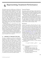
STA2 Cell 4 Estimate
FIGURE 23.12 The capital cost for FWS wetlands as a function of size (N  84 wetlands). Points for A  300 m
2
were excluded from the
regression. C  194 A
0.690
; R
2
 0.79; C in 1,000s of dollars.
1
10
100
1,000
10,000

0.001 0.01 0.1 1 10 100
Area (ha)
Cost (thousands of dollars)
HSSF
Regression
FIGURE 23.14 The capital cost for HSSF wetlands as a function of size (N  63 wetlands). C  652 A
0.704
; R
2
= 0.75; C in 1,000s of dollars.
FIGURE 23.13 The capital cost for FWS wetlands as a function of ow rate (N  61 wetlands). Points for Q  1 m
3
/d are not considered in
the regression. C  518Q
0.729
; R
2
 0.79; Q and C in 1,000s of dollars.
1
10
100
1,000
10,000
100,000
1,000,000
0.0001 0.001 0.01 0.1 1 10 100 1,000 10,000
Flow (1,000 m
3
/d)
Capital Cost (thousands of dollars)

FWS
Regression
One ha Example
STA2 Cell 4 Estimate
© 2009 by Taylor & Francis Group, LLC
Economics 809
The result of the nearly identical exponents for area is a nearly
xed ratio of costs for FWS and HSSF systems over the range
of areas where both are used (about 0.1–10 ha). That ratio is
3.32 ± 0.14, with HSSF being the more expensive. The litera-
ture contains several estimates of the median cost per hectare
for FWS and HSSF wetlands. For the data reviewed here,
these medians are $98,000/ha for FWS and $1,230,000/ha
for HSSF systems. These unit costs are not usable in a com-
parison, because they cover entirely different size ranges. As
detailed in Chapter 16, treatment per unit area is about the
same for FWS and HSSF systems, and as seen here HSSF
costs are about triple those for the equivalent FWS system.
A direct comparison of costs on a ow basis is inap-
propriate, because FWS and HSSF systems are generally
designed for different pollutants and different removals.
These cost functions may be used to obtain an approxi-
mate cost for a prospective project, but should not be used in
lieu of detailed cost estimation.
In many cases, for domestic wastewater treatment, the
measure of HSSF wetland size is the population served, partly
because only design ows are known and partly because the
cost to the individuals served is the desired result. Some
results reported in the literature are:
HSSF (Central America): PE R

2
C 360 0 97
0 755.
.
Platzer et al. (2002) (23.5)
HSSF (Spain): PE R
2
C 490 0 71
0 707.
.
Nogueira et al. (2006) (23.6)
HSSF (Portugal): PE estimatedC  2 200
0 679
,
.
Junca de Morais et al. (2003) (23.7)
where
PE Population equivalent
Cost, 2006 U

C SSD
The high regional variability is apparent in these relations.
No matter which measure of scale is used, it is clear that
an exponent of something like 0.7 is appropriate for scaling
of these continuous ow systems.
Stormwater systems present a different situation, because
the wetland size is often determined from the watershed size,
and not any specic performance specication. Scaling to
the size of the watershed may then be more appropriate
(Wossink and Hunt, 2003). For the state of North Carolina,

the following cost function has been derived by Wossink and
Hunt (2003):
Stormwater wetlands C  6 910
0 484
,
.
WS 1 < WS < 100
(23.8)
where
WS Watershed area, ha
Cost, 2006 USD

C
This amounts to a set of formulas when converted to wet-
land area, because the guidelines for sizing in North Carolina
specify wetland to watershed area ratios (WWARs) of
between 1.0 and 6.5%.
23.2 OPERATION AND MAINTENANCE COSTS
Wetland systems have very low intrinsic O&M costs, includ-
ing pumping energy, compliance monitoring, maintenance
of access roads and berms, and mechanical component
repair. These basic costs are much lower than those for com-
peting concrete and steel technologies, by a factor of 2–10.
Attempts at harvesting, or at maintenance of a particular
vegetation species composition, can prove costly. Ancil-
lary research costs—which can occur at the directive of the
regulatory agencies—have sometimes cancelled out this
large potential advantage, especially for natural treatment
wetlands. Most maintenance tasks associated with operating
a wetland facility deal with servicing pump headworks, and

other conventional components of the treatment plant (U.S.
EPA, 2000a).
1
10
100
1,000
10,000
0.1 1 10 100 1,000 10,000 100,000
Flow (m
3
/d)
Cost (thousands of dollars)
HSSF
Regression
FIGURE 23.15 The capital cost for HSSF wetlands as a function of ow rate (N  58 wetlands). C  18Q
0.498
; R
2
 0.76; C in 1,000s of dollars.
© 2009 by Taylor & Francis Group, LLC
810 Treatment Wetlands
FREE WATER SURFACE WETLANDS
The O&M costs for a FWS facility include pumping energy,
compliance monitoring, dike maintenance, and equipment
replacement and repairs. Dike maintenance consists of mow-
ing and preservation of structural integrity. Equipment re-
placement and repairs pertain to piping and pipe supports,
structures, and pumps. Pumping energy may be accurately
quantied, as can the initial level of compliance monitor-
ing, once a permit is issued. Mowing is primarily a matter

of aesthetics, with secondary emphasis on visual detection of
snakes and alligators. If public use is encouraged, there may
be a need to maintain signage, trails, and boardwalks. Nui-
sance control or removal may be required, most often target-
ing mosquitoes, burrowing rodents, and bottom-stirring sh.
Nuisance control, such as mosquito and rodent eradication,
has sometimes proved to be troublesome.
The sum total of these activities is usually relatively
inexpensive. No chemical purchases are involved, and there
is not a need for highly trained personnel, nor signicant
time requirements for the necessary semiskilled employees.
Annual costs range from $5,000 to $50,000 per year for small
systems. However, ancillary research can greatly increase
these expenditures. The estimate for the Incline Village sys-
tem, made at the time of nal conceptual design, was $163,000
per year (Table 23.12).
Permit-related sampling and reporting, combined with
maintenance of upstream and downstream treatment pro-
cesses, constitute most of the routine O&M associated
with FWS wetlands. At Arcata, California, it has been esti-
mated that O&M tasks directly associated with the wetlands
require about $1600/ha·yr when adjusted to 2006 USD (U.S.
EPA, 2000a). These types of routine checks do not include
muskrat or nutria removal, or mosquito control, which will
increase operating costs. Costs for these types of animal or
vector control activities are highly site specic in nature,
and are generally best estimated by assessing the amount of
operator labor involved plus the cost of any control agents
or equipment.
The limited amount of FWS O&M data from the litera-

t
u
re is presented in Figure 23.16, and shows a median cost of
about $2,000/ha.
SUBSURFACE FLOW WETLANDS
One primary operating cost of a single-home HSSF system is
the cost associated with pumping the septic tank. Other costs
are mainly determined by local permit requirements, which
vary widely across the United States. In western Ohio, the
annual maintenance and monitoring costs are approximately
$250/yr when adjusted to 2006 costs (Steer et al., 2003). Many
systems are permitted at the state or provincial level, and are
required to have licensed operators submit monthly discharge
monitoring reports. An example of the cost breakdown for an
HSSF system is shown in Table 23.13. Most of the O&M is
associated with permit-related sampling and correspondence,
followed by management of pumps, septic tanks, control
TABLE 23.12
Estimated O&M Costs for the 135-ha Incline Village
FWS Wetland System
Item Annual Cost ($)
Personnel 95,315
Energy 4,766
Monitoring 40,032
Maintenance materials 22,876
Total 162,988
Note: This
information was developed after the conceptual design was
nalized.
It does not include research costs, nor prots derived from

hunter use charges. Costs are in 2006 USD. O&M  operation and
maintenance.
Source: Data from
CWC (1983) Draft Design Memorandum, Incline
Village General Improvement District Wetlands. Culp, Wesner, and Culp
(CWC): 3461 Robin Lake, Cameron Park, California.
y x&









   
!#$%"
" $
FIGURE 23.16 Operation and maintenance (O&M) costs for FWS wetlands (N  21).
© 2009 by Taylor & Francis Group, LLC
Economics 811
panels, and other conventional treatment components. For
small-scale systems, it is not meaningful to project per-hectare
O&M costs because small HSSF systems have essentially the
same monitoring and reporting requirements as large systems.
For larger systems, it is possible to separate wetland O&M
from total O&M required, including the rest of the facility.
The annual O&M expenses for the HSSF wetland at Carville,
Louisiana (568 m

3
/d, 0.26 ha), were estimated at $780/yr or
$3,000/ha.yr (U.S. EPA, 2000a) (2006 USD). This is approxi-
mately 6% of the O&M budget for the entire treatment system.
Inlet zone maintenance has the potential to be a large com-
ponent of HSSF maintenance costs. Inlet zone maintenance
will depend on the remedy method selected (replacement,
washing, or chemical cleaning; none of these procedures have
been used widely to x clogged HSSF wetlands). Also, the
time interval between bed maintenance is a factor. To date,
no rational methods to predict bed clogging have been devel-
oped, although it is apparent that it is a widespread problem
in full-scale HSSF wetlands (Cooper et al., 2006a).
Here, we will consider the potential economic con-
sequences of inlet zone maintenance. In the example of
Table 23.13, it was assumed that inlet zone maintenance
would be 15% of the construction cost, and inlet zone main-
tenance would occur every ve years. These assumptions are
based on the very limited data presented in Table 22.6. Based
on these assumptions, and Equation 23.2, the cost for inlet
zone maintenance every ve years is predicted at $20,438
(2006 USD); at a 5% interest rate, the annual cost is $3,698.
The assumption parameters (time to clog, percentage of con-
struction costs) can, however, vary. It is apparent at this stage
of technology development that inlet zone clogging is likely
to be the largest maintenance cost component associated
with HSSF wetlands. When evaluating the cost-effectiveness
of any future projects, inlet zone maintenance costs must be
considered. The continued viability of HSSF wetlands as an
economically efcient technology is dependent on nding a

cost-effective solution to the clogging problem.
23.3 PRESENT WORTH ANALYSES
The capital costs for a wetland project are “up front” needs,
typically expended in the rst year of the project. In contrast,
the O&M costs are recurring, with a need for expenditure in
every year of operation. Thus, when evaluating alternatives or
planning for nancing, it is necessary to combine these two
types of costs to obtain a true picture of the overall project
cost. Two basic choices are available. The rst is to convert
the future time stream of O&M costs to an amount of money
that one would need to put in the bank to pay for the future
O&M, and add it to the initial capital investment. This proce-
dure produces the present worth of the project (Humphreys,
1991). The second choice is to convert the initial capital invest-
ment into a time series of payments that may be added to the
time series of O&M costs, to create an annualized project
cost. In essence, the capital cost is borrowed, and repaid over
time. It is this latter approach that is often used for nancing
wastewater treatment projects. In fact, in the United States, a
homeowner may well be paying the two bills separately each
month: one payment to pay off the debt on building the sys-
tem, and a second to pay for operating costs. Unfortunately,
only a very few literature sources deal with the combination
of both types of project costs for treatment wetlands.
Treatment wetlands are distinctively different from
mechanical plants in a few very important ways. It is therefore
necessary to examine the basic elements of the accumulation
of costs, and for simplicity we here consider only the present
worth analysis. However, it is a relatively simple matter to
weave these concepts into an annualized cost analysis. Over

the life of the project, in a simplied sense, it is expected that
the following costs will be incurred:
Capital costs, both direct and indirect, usually in
the rst year of the project life.
Annual O&M costs. These include monitoring and
other routine activities.
Periodic, nonannual costs. These might include
sediment cleanout, for instance.
End of project costs and values, sometimes termed
“salvage values.” These may include not only
demolition and disposal costs, but also the resale
value of project assets.
The preceding sections have detailed the costs in the rst two
categories (capital and O&M).
•
•
•
•
TABLE 23.13
Example Annual Operational Costs for a 46-Home
Residential Development in Minnesota
Monitoring Cost ($)
Sample collection 4,320
Lab coordination 364
Analytical 1,405
Regulatory correspondence 573
Permit renewal 2,166
Subtotal 8,828
O
per

ating
Visual monitoring 1,353
Electric 3,596
Telephone 521
Septic tank pumping 1,249
Subtotal 6,719
Maintenance
Equipment replacement 2,320
Equipment maintenance 521
Emergency repairs 521
Sewer maintenance 1,041
Inlet zone bed maintenance 3,698
Subtotal 8,101
O
v
erhead
Billing 1,437
Total 25,085
Note: Costs
are in 2006 USD. Note that the inlet zone of the wetland bed
line item accounts for nearly 50% of the maintenance cost.
© 2009 by Taylor & Francis Group, LLC
812 Treatment Wetlands
PRESENT WORTH CONCEPTS
The total cost of a project at the time of inception is the total
of capital costs, engineering services, and the present worth
of O&M costs over the project life. This approach to eco-
nomic estimating is required when the alternatives under
consideration vary greatly in their life expectancy, and in
their O&M costs. This is the case for wetlands. The overall

project evaluation requires consideration of both capital and
O&M costs, and the present worth technique is the appro-
priate vehicle for combining the two. The present worth of
O&M costs, including equipment repairs and replacements,
is the money that needs to be set aside now, at the prevailing
interest rate, to pay for these future costs.
It is not possible to anticipate all the project-specic
details of the economics of treatment wetlands. However,
there are certain common features of many projects that are
considered here.
Discount Rate
The time value of money reects the interest on borrowed
sums and the ination rate. The discount rate used in pres-
ent worth calculations is the excess of the interest rate over
ination. In treatment wetland evaluations, discount rates of
4–8% are commonly used.
Life
Expectancy
Traditionally, the life expectancy of a “conventional” treat-
ment alternative is 20 years. A treatment wetland has a longer
life expectancy than concrete and steel equipment. Although
there are no examples of engineered systems with long periods
of operation, there are long-lived FWS wetland systems that
have retained their effectiveness for up to 80 years, based on
ex post facto monitoring. Both the Brillion Marsh, Wisconsin
(Spangler et al., 1976b), and Great Meadows Marsh, Mas-
sachusetts (Yonika et al., 1979), operated for over 70 years,
a
nd in later years were shown to have retained treatment ef-
ciency. As fully functional ecosystems, treatment wetlands

may be expected to sustain their character for as long as
appropriate hydrology is maintained. It is early in the his-
tory of constructed wetland facilities, so there is not a long
track record on life expectancies for wetland components.
However, in general terms, pumps and piping may last on the
order of 40 years, and repair frequencies are known. Berms,
dikes, and levees have lives in excess of 50 years. Therefore,
it is plausible that treatment wetlands should be ascribed a
basic life of 40–50 years, with mechanical components being
replaced at greater frequency.
Present Worth of Future One-Time Costs
The amount of money needed for a future expenditure reects
the discount rate in a simple, compound interest sense:
PS
i
m


1
1()
(23.9)
where
discount rate, fraction per year
ye
i
m

 aars before need
present value, $
future

P
S

 aamount, $
Thus a $1,000 pump replacement ten years from now will
require $614 today if the discount rate is 5%.
Present Worth of Future O&M
Many O&M costs occur as a continuing stream. In analysis,
it is usual to aggregate these into a yearly amount, and then
to compute the sum of all such future payments. This may
be done sequentially using Equation 23.9, or the sum can be
directly evaluated from
PY
i
ii
YF
N
N




()
()
11
1
pw
(23.10)
where
discount rate, fraction per year

pw
i
F

 ppresent value factor, dimensionless
lifeN  eexpectancy, yr
present value, $
yearly a
P
Y

 mmount of O&M, $
Thus, the median FWS O&M of $2,000/ha·yr (Figure 23.16),
over a 50-year lifetime, will require $36,512 today if the
discount rate is 5%. Note that payment number 50 requires
only $174 of today’s money.
Salvage Values and Decommissioning Costs
It is common practice to claim no salvage value at the end of
project life in a feasibility study for mechanical plants; but
this does not make sense in the context of a wetland project.
Typically, the entire acquisition price is charged to the project
up
front, and there is no “salvage” value at the end of 20 years.
In contrast to the crumbling concrete and rusted steel left after
the mechanical process reaches the end of its useful life, the
land associated with the wetland project will probably have
greater (or equal) value than that at the time of acquisition.
This principal component of the wetland project will probably
have appreciated in value. It may be more accurate to delete
land cost from the comparison for that reason. Investments

in land are not subject to normal wear-out and replacement
charges in a long-term view of the project economics. There-
fore, the “salvage” value of the wetland property, which may
have appreciated over the project life, is typically much higher
than that of a mechanical plant, which may have depreciated.
The present worth of the land after the nominal project life
should be included as a credit in economic evaluation if com-
parisons are being made. These end-of-life costs and values
are brought to present-day dollars by use of the present worth
factor for the last year of the project.
© 2009 by Taylor & Francis Group, LLC
Economics 813
Total Present Worth
The various costs, consisting of capital plus the present worth
of O&M, various replacement costs, and salvage values, are
combined to yield the total present worth of the project. Thus,
the example project in Table 23.8 (1 ha), with no replacements
or equipment salvage, would yield at 5% discount rate and a
50-year life:
Capital cost $480,000
Present worth of O&M $36,512
Present worth of nal land value $10,000
Total present worth $506,512
An Illustration
An alternative comparison is illustrated in Table 23.14, evaluat-
ing wetland treatment and chemical treatment to remove phos-
phorus from agricultural runoff water in southern Florida. The
dollar values in this example are large, because it is based on a
system for the treatment of a very large ow (≈760,000 m
3

/d).
The estimates in this table were developed from information
available at the time of nal conceptual design, and are subject
to change during nal design and the accompanying modi-
cations. The example is included here to illustrate the unique
features of evaluating wetland alternatives.
The chemical treatment alternative is 17% cheaper than
the treatment wetland on the basis of the capital expenditures
needed to build the project. On the surface, this makes chem-
ical treatment the more attractive alternative. This up-front
comparison presumes a life span short enough that equipment
does not need to be replaced, nominally 20 years. However, if
the life span of the project is taken to be 50 years—which is
characteristic of constructed wetlands, and has been demon-
strated in the region—the analysis changes. It becomes nec-
essary to consider the salvage value of worn out components,
a
n
d their replacement costs. In Table 23.14, it is assumed that
worn out equipment has zero value: it is unsalable, and there
is no charge for disposal. On the other hand, land acquired for
the project is assumed to maintain its value; no replacement
purchases are necessary. It is therefore logical to exclude land
costs from the analysis, because it can be sold at the conclu-
sion of the project with no loss in value.
When these factors are taken into consideration, the treat-
ment wetlands are 13% cheaper than chemical treatment. The
conclusion of the capital cost analysis is reversed.
Next, the O&M costs are totaled and converted to their
present worth. Chemical treatment, as the name implies,

requires more energy, materials, labor, and supplies than
wetland treatment. Monitoring costs would be the same. In
this example, and in virtually all similar cases, O&M costs
are higher for the equipment-oriented technology. The annual
O&M for chemical treatment is twice as expensive. The pres-
ent worth of O&M is a signicant fraction of the project cost.
Consequently, the total present worth of the wetlands project
is only 70% of the total present worth of the chemical treat-
ment alternative.
TABLE 23.14
Estimated Cost Comparison for Phosphorus Reduction in Agricultural Runoff (in Thousands of Dollars)
Wetland Alternative Chemical Treatment Alternative
Total Capital Costs Excluding Replacement 193,028 Total Capital Costs Excluding Replacement 160,331
Land 51,228 Land 3,184
Procurement premium 15,368 Procurement premium 558
Pump station capital cost 21,256 Replaceable equipment
Mixing through thickening 76,454
Equipment replacement (present worth, 8% discount rate) Equipment replacement (present worth, 8% discount rate)
Pump station replacement
(25% pump station capital replaced @ 25 years) 777
Pumps piping electrical (25% @ 25 years)
Mixing through thickening (100% @ 20 and 40 years)
1,015
2,898
Land-Free Capital Cost 142,577 Land-Free Capital Cost 161,060
Operating and Maintenance Costs Operating and Maintenance Costs
Labor 881 Labor 1,577
Materials 184 Materials 372
Chemicals 0 Chemicals 833
Energy 339 Energy 339

Monitoring 223 Monitoring 223
Total annual O&M 1,628 Total annual O&M 3,704
Present Worth of O&M (50-year life span, 8%) 49,754 Present Worth of O&M (50-year life span, 8%) 113,294
Total Present Worth of Capital  O&M
192,330
Total Present Worth of Capital  O&M
276,175
Source: Base
information
from Brown and Caldwell (1993) Phase II Evaluation of Alternative Treatment Technologies. Report to the South Florida Water
Management District, 18 February 1993.
© 2009 by Taylor & Francis Group, LLC
814 Treatment Wetlands
The assumed factors in this example will not prevail
in all circumstances, but it does serve to indicate that extra
care should be taken in economic analysis of a wetland
alternative.
ANNUALIZED COST
This procedure has all the same elements as present worth,
but the total project costs are allocated to a uniform series of
annual payments over the life of the project. In simplest terms,
a loan for the initial capital investment is repaid over the life
of the wetland, and added to the annual O&M charges. This
total annualized cost becomes the basis for comparison. For
example, the capital costs for the project in Table 23.13 were
$513,515 (2006 USD). At a 5% discount rate and 20-year life,
the annual repayment would be $41,206. The O&M is $21,386
per year, and thus the total annualized cost is $62,592.
Another situation in which an annualized cost approach
may be warranted is in the calculation of sewer bills. In the

United States, homes are typically billed for sewer service on
a quarterly or monthly basis. Funds are accumulated and used
to pay off debt associated with capital costs, routine mainte-
nance, emergency repairs, and component replacement. An
example of this type of rate calculation for a 53-home treat-
ment system is shown in Table 23.15; the associated cash ow
is shown in Figure 23.17.
Annualization has also been applied to urban stormwa-
ter wetlands in North Carolina (Wossink and Hunt, 2003).
For watersheds of 6–20 ha, annual costs were found to be
$22,000–$85,000/ha, depending upon the (irrecoverable)
value ascribed to land. Those land values were taken to be
$125,000/ha for undeveloped residential land, and $540,000/
ha for land in commercial development zones. Wetland
watershed area ratios of 1.0–6.5% were applied, on a region-
ally variable basis.
Cost per Pollutant Load Removed
It is sometimes appropriate to measure the cost of a proj-
ect, not in terms of the population served or the hectares
required, but per-unit mass of pollutant removed. This may
be done by dividing the cost by the removal. For instance,
phosphorus removal in the Florida Everglades wetland
projects has been assessed in terms of the present worth of
dollars required divided by the lifetime total mass of phos-
phorus removed in kilograms. For a discount rate of 8% and
a lifetime of 20 years, the present worth for removing an
estimated 157,000 kg of phosphorus per year for 20 years
was $81,000,000, or about $26/kg.
The concept of nutrient credit trading, coupled with the
land needed for treatment wetlands, has spurred consider-

ation of the use of off-site wetlands to remove nitrogen and
phosphorus rather than on-plant-site mechanical equipment
(Hey et al., 2005). The loads that need to be removed at large
wastewater treatment plants are easily identied, as can the
costs of such nutrient removal at the plant. Therefore, the
wetland alternative needs to be evaluated on the basis of cost
per kilogram of nitrogen and phosphorus. FWS treatment
wetlands are more economical than traditional removal (Hey
et al., 2005).
ECONOMICS OF STORAGE
Cold climate conditions may engender the need for winter
storage of wastewater. Overland ow systems require stor-
age whenever the mean daily temperature is below freezing
(Crites et al., 2006), but FWS constructed wetlands have a
wider operating window. For example, storages for northern
wetlands are 180 days at Minot, North Dakota; Houghton
Lake, Michigan; and Estevan, Saskatchewan. However, stor-
age may be as much as 320 days in the arctic (Dillon Consult-
ing, Ltd., 2006).
The use of winter storage avoids the “bottleneck” winter
period, when some wetland processes are operating at their
slowest pace. As discussed in Chapter 17, this period may
be avoided if a storage pond is available, or is constructed.
There are several competing factors that must be considered
in the evaluation of alternatives. First, if the wetland is to
operate in winter, the area needed will be larger than that
needed in warm conditions. The area factor is on the order
of three, meaning that the winter size will be about triple
the summer size to accomplish the same degree of treatment
for the same ow. This corresponds to a temperature coef-

cient of about Q 1.07, and a temperature difference of 16°C
(mean summer 18°C, mean winter 2°C). Second, the ow is
not the same if storage is added; the entire year’s ow must
be disposed of during the warm season. For instance, if six
months’ storage is employed, then the warm season ow will
be double the annual average. Therefore, the wetland size is
reduced according to the warmer temperatures, but increased
to account for the increased ow. Nevertheless, the size of
the wetland will decrease if storage is added. Third, the stor-
age pond, however, adds to the overall project footprint, thus
increasing land and liner costs. In general, there is only a
small difference in total area for storage periods of 90 days,
but a signicant increase (≈70%) in total project area for 180
days of storage, compared to year-round operation with a
large wetland to deal with the winter bottleneck. Fourth, the
amount of earthmoving increases, nearly in direct proportion
to the volume of water being treated (for level sites).
An
Il
lustration
As an illustration, consider a system to be constructed on a
level site, with a (square) storage pond and a square wetland
outline, which may have internal compartments and parallel
o
w paths (Figure 23.18). The further assumptions are:
The design hydraulic loading during the warm
season is 5 cm/d. If storage is used, this loading
rate prevails on average throughout the discharge
(warm) season, and determines the required area.
The design hydraulic loading during the cold sea-

son is 1.25 cm/d. If the wetland is to be used year-
round, this determines the required area.
•
•
© 2009 by Taylor & Francis Group, LLC
TABLE 23.15
Example of a Rate Structure Calculation Using the AccuRate Financial Planning Software (in Dollars)
AccuRate Financial Planning Software
Including capital replacement
Total revenue 1,133,704
Total expense 1,108,704
Net 25,000.00
Year
2007 2008 2009 2010 2011 2012 2013 2014 2015 2016 2017
Revenue
Monthly rate per home 42.91 43.76 44.64 45.53 46.44 47.37 48.32 49.29 50.27 51.28 52.30
Occupied homes 12 25 50 53 53 53 53 53 53 53
SAC fee 1,200 1,200 1,200 1,200 1,200 1,200 1,200 1,200 1,200 1,200 1,200
SAC revenue 14,400 15,600 30,000 3,600
0 000000000
Subtotal Revenue 20,578 28,729 56,784 32,559 29,538 30,129 30,731 31,346 31,973 32,612 33,264
Expenses

Monitoring (service provider cost) 14,300 14,586
14,878 15,175 15,479 15,788 16,104 16,426 16,755 17,090 17,432
Operating costs 7,020 7,160 7,304 7,450 7,599 7,751 7,906 8,064 8,225 8,390 8,557
Maintenance costs 3,450 3,519 3,589 3,661 3,734 3,809 3,885 3,963 4,042 4,123 4,206
Capital replacement 0 801 520 1,455 3,240 1,414 5,992 1,565 580 4,466
Subtotal Expenses 24,770 26,066 26,291 27,741 30,052 28,762 33,887 30,018 29,602 34,069 30,194


Net (4,192) 2,663 30,493 4,818 (514) 1,367 (3,156) 1,328 2,371 (1,457) 3,070
Interest (83.83) 53.26 609.86 96.35 (10.28) 27.34 (63.12) 26.56 47.41 (29.13) 61.40
Cash in Bank
4,275 1,559
29,544 34,458 33,934 35,328 32,109 33,464 35,882 34,396 37,527
Replacement
Annual Asset Replacement
Manufacturer
Cost
I
nstallation
Labor
I
ncidental
Costs
Cost
(today)
Schedule
(years) 2007 2008 2009 2010 2011 2012
Collection
Lift station control panel parts 400 100 0 500 3 0 0 520 0 0
Lift station pump replacement 2,000 650 25 5,350 7 0 0 0 0 0
Sewer repair 500 10,000 5,000 15,500 25 0 0 0 00000
Tr
eatment
Constructed Wetland
Pump replacement 1,500 200 25 0 7 0 0 0 00000
Piping repair 100 350 0 450 15 0 0 0 00000
Blower replacement 750 350 75 588 4 0 0 0 623000
Disinfection

UV Disinfection
Bulb replacement 600 160 25 785 2 0 801 0 832 0
Permitting
Permitting improvements 2,500 500 0 3,000 5 0 0 0 0 3,240000
Subtotal
0 801 520 1,455 3,240 1,414
Note: Revenue is received from monthly sewer bills and in the early years of the project, se
wer connection fees. Funds are expended to operate the system and replace w
orn-out components.
© 2009 by Taylor & Francis Group, LLC
816 Treatment Wetlands
The soils on the site are acceptable for berms, and
thus cut and ll may be balanced. This is presumed
for pond and wetland individually.
Setbacks around the project are 20% of the bermed
areas.
The berms have 3:1 side slopes, and a 3-m top width.
The storage pond requires a 0.5-m freeboard and
a 0.5-m minimum depth. The operating depth
change is to be 2 m. Thus, the total depth of the
basin is 3 m.
The wetland requires a 1-m freeboard (to allow
for solids accumulation and depth increases) and
a 0.3-m average depth. Thus, the total depth of the
basin is 1.3 m.
Wetland internals, meaning inlet and outlet deep
zones and cell divider berms, are not considered.
•
•
•

•
•
•
The results of cut-and-ll calculations are given in Table 23.16,
for three ow rates (10, 100, and 1,000 m
3
/d), and for 0, 90,
and 180 days of storage. Even though this is a highly simpli-
ed illustration, several important issues can be identied.
First, the increased summer ows partially balance the higher
area requirements for winter operation. This results in a wet-
land size of one third to half the winter size, not a reduction
to one fourth as the loading implies. The earth moved is in
the range of 0.4–1.2 m
3
/m
2
of the total bermed area. The total
project area increases with the addition of storage, but only
minimally for 90 days. In general, 90 days of storage means
less earthmoving than for zero storage, and 180 days does not
require much more. The nature of the cut and ll is such that
the wetland water surface is near the original ground eleva-
tion (−0.29 to 0.09 cm). However, the maximum pond water
elevation is above the original grade (0.43–2.09 m).
$50,000
$40,000
$30,000
$20,000
$10,000

$0
–$10,000
Cash in Bank
2007
2008
2009
2010
2011
2012
2013
2014
2015
2016
2017
2018
2019
2020
2021
2022
2023
2024
2025
2026
2027
2028
2029
2030
2031
2032
2033

2034
2035
Cash in Bank
Recommended Capacity
FIGURE 23.17 Example of cash-ow projection for a 53-home treatment wetland system based on the user rate structure of Table 23.15,
using AccuRate nancial planning software.
Project site
Setback
Wetland bottom
Inner berm slope
Top of berm
Fence
Outer berm slope
FIGURE 23.18 General layout of a treatment wetland. For a small system, the overall project footprint is much larger than the wetted area.
© 2009 by Taylor & Francis Group, LLC
Economics 817
This illustration is not intended to be used in design,
because of the highly restrictive assumptions. However, mod-
ern computer-aided design tools are capable of easily dealing
with irregular sites, more general basin geometries, and wet-
land internals.
Economics vary from location to location. The relative
costs of land and earthmoving combine with the size and
volume calculations to provide a basis for alternative selec-
tion. In the event that costs of storage or no storage are com-
petitively close, the choice to avoid winter operation is likely
to be more attractive. Additionally, controlled discharge
strategies can modify the storage and wetland requirements
as detailed in Chapter 17. The treatment potential of the
combination is evaluated for the wetland (using the proce-

dures in this book) and lagoon (from other sources) perfor-
mance calculations.
TABLE 23.16
Effects of Storage on Project Areas and Earthmoving for Hypothetical Site Conditions
a
Wetland Wetted
Area (m
2
)
Wetland Earth
Moved (m
3
)
Storage
Volume (m
3
)
Storage Top
Area (m
2
)
Storage Earth
Moved (m
3
)
Project Total
Area (m
2
)
Total Earth

Moved (m
3
)
10 m
3
/d
No storage 800 1,207 0 0 0 2,332 1,207
90 days 265 446 900 896 708 3,204 1,154
180 days 395 634 1,800 1,505 1,280 4,681 1,914
100
m
3
/d
No storage 8,000 10,901 0 0 0 13,852 10,901
90 days 4,705 3,745 9,000 5,775 4,666 14,459 8,411
180 days 3,946 5,485 18,000 10,775 7,776 25,555 13,261
1,000
m
3
/d
No storage 80,000 105,557 0 0 0 109,428 105,557
90 days 26,545 35,411 90,000 48,887 22,820 105,094 58,231
180 days 39,459 52,394 180,000 95,469 34,852 187,883 87,246
a
See text for conditions and assumptions.
SUMMARY
Despite the inherent variability in costing a wetland treat-
ment system, basic cost components of a wetland can be
estimated using a line-item approach. Wetland treatment
systems generally share a basic list of common components,

which usually includes items such as land, earthwork, liner,
rooting medium, wetland plants, and hydraulic control struc-
tures. The cost of these basic components can be estimated
using pricing and availability information for a given regional
economy. However, the line-item approach makes estimating
economies of scale difcult, and has limited application in
areas in which local pricing information is unavailable. Other
components of wetland system design, such as site investiga-
tion, engineering design fees, and operation and maintenance
(O&M) costs, should also be included when developing an
overall cost estimate.
© 2009 by Taylor & Francis Group, LLC