- Trang chủ >>
- Khoa Học Tự Nhiên >>
- Vật lý
analytical mechanics an introduction jun 2006
Bạn đang xem bản rút gọn của tài liệu. Xem và tải ngay bản đầy đủ của tài liệu tại đây (2.96 MB, 788 trang )
Analytical Mechanics
This page intentionally left blank
Analytical Mechanics
An Introduction
Antonio Fasano
University of Florence
Stefano Marmi
SNS, Pisa
Translated by
Beatrice Pelloni
University of Reading
1
3
Great Clarendon Street, Oxford OX2 6DP
Oxford University Press is a department of the University of Oxford.
It furthers the University’s objective of excellence in research, scholarship,
and education by publishing worldwide in
Oxford New York
Auckland Cape Town Dar es Salaam Hong Kong Karachi
Kuala Lumpur Madrid Melbourne Mexico City Nairobi
New Delhi Shanghai Taipei Toronto
With offices in
Argentina Austria Brazil Chile Czech Republic France Greece
Guatemala Hungary Italy Japan Poland Portugal Singapore
South Korea Switzerland Thailand Turkey Ukraine Vietnam
Oxford is a registered trade mark of Oxford University Press
in the UK and in certain other countries
Published in the United States
by Oxford University Press Inc., New York
c
2002, Bollati Boringhieri editore, Torino
English translation
c
Oxford University Press 2006
Translation of Meccanica Analytica by Antonio Fasano and
Stefano Marmi originally published in
Italian by Bollati-Boringhieri editore, Torino 2002
The moral rights of the authors have been asserted
Database right Oxford University Press (maker)
First published in English 2006
All rights reserved. No part of this publication may be reproduced,
stored in a retrieval system, or transmitted, in any form or by any means,
without the prior permission in writing of Oxford University Press,
or as expressly permitted by law, or under terms agreed with the appropriate
reprographics rights organization. Enquiries concerning reproduction
outside the scope of the above should be sent to the Rights Department,
Oxford University Press, at the address above
You must not circulate this book in any other binding or cover
and you must impose the same condition on any acquirer
British Library Cataloguing in Publication Data
Data available
Library of Congress Cataloging in Publication Data
Fasano, A. (Antonio)
Analytical mechanics : an introduction / Antonio Fasano, Stefano Marmi;
translated by Beatrice Pelloni.
p. cm.
Includes bibliographical references and index.
ISBN-13: 978–0–19–850802–1
ISBN-10: 0–19–850802–6
1. Mechanics, Analytic. I. Marmi, S. (Stefano), 1963- II. Title.
QA805.2.F29 2002
531
.01—dc22 2005028822
Typeset by Newgen Imaging Systems (P) Ltd., Chennai, India
Printed in Great Britain
on acid-free paper by
Biddles Ltd., King’s Lynn
ISBN 0–19–850802–6 978–0–19–850802–1
13579108642
Preface to the English Translation
The proposal of translating this book into English came from Dr. Sonke Adlung
of OUP, to whom we express our gratitude. The translation was preceded by hard
work to produce a new version of the Italian text incorporating some modifications
we had agreed upon with Dr. Adlung (for instance the inclusion of worked out
problems at the end of each chapter). The result was the second Italian edition
(Bollati-Boringhieri, 2002), which was the original source for the translation. How-
ever, thanks to the kind collaboration of the translator, Dr. Beatrice Pelloni, in the
course of the translation we introduced some further improvements with the aim of
better fulfilling the original aim of this book: to explain analytical mechanics (which
includes some very complex topics) with mathematical rigour using nothing more
than the notions of plain calculus. For this reason the book should be readable by
undergraduate students, although it contains some rather advanced material which
makes it suitable also for courses of higher level mathematics and physics.
Despite the size of the book, or rather because of it, conciseness has been a
constant concern of the authors. The book is large because it deals not only with
the basic notions of analytical mechanics, but also with some of its main applica-
tions: astronomy, statistical mechanics, continuum mechanics and (very briefly)
field theory.
The book has been conceived in such a way that it can be used at different levels:
for instance the two chapters on statistical mechanics can be read, skipping the
chapter on ergodic theory, etc. The book has been used in various Italian universities
for more than ten years and we have been very pleased by the reactions of colleagues
and students. Therefore we are confident that the translation can prove to be useful.
Antonio Fasano
Stefano Marmi
This page intentionally left blank
Contents
1 Geometric and kinematic foundations
of Lagrangian mechanics 1
1.1 Curves in the plane 1
1.2 Length of a curve and natural parametrisation 3
1.3 Tangent vector, normal vector and curvature
of plane curves 7
1.4 Curves in R
3
12
1.5 Vector fields and integral curves 15
1.6 Surfaces 16
1.7 Differentiable Riemannian manifolds 33
1.8 Actions of groups and tori 46
1.9 Constrained systems and Lagrangian coordinates 49
1.10 Holonomic systems 52
1.11 Phase space 54
1.12 Accelerations of a holonomic system 57
1.13 Problems 58
1.14 Additional remarks and bibliographical notes 61
1.15 Additional solved problems 62
2 Dynamics: general laws and the dynamics
of a point particle 69
2.1 Revision and comments on the axioms of classical mechanics . 69
2.2 The Galilean relativity principle and interaction forces 71
2.3 Work and conservative fields 75
2.4 The dynamics of a point constrained by smooth holonomic
constraints 77
2.5 Constraints with friction 80
2.6 Point particle subject to unilateral constraints 81
2.7 Additional remarks and bibliographical notes 83
2.8 Additional solved problems 83
3 One-dimensional motion 91
3.1 Introduction 91
3.2 Analysis of motion due to a positional force 92
3.3 The simple pendulum 96
3.4 Phase plane and equilibrium 98
3.5 Damped oscillations, forced oscillations. Resonance 103
3.6 Beats 107
3.7 Problems 108
3.8 Additional remarks and bibliographical notes 112
3.9 Additional solved problems 113
viii Contents
4 The dynamics of discrete systems. Lagrangian formalism 125
4.1 Cardinal equations 125
4.2 Holonomic systems with smooth constraints 127
4.3 Lagrange’s equations 128
4.4 Determination of constraint reactions. Constraints
with friction 136
4.5 Conservative systems. Lagrangian function 138
4.6 The equilibrium of holonomic systems
with smooth constraints 141
4.7 Generalised potentials. Lagrangian of
an electric charge in an electromagnetic field 142
4.8 Motion of a charge in a constant
electric or magnetic field 144
4.9 Symmetries and conservation laws.
Noether’s theorem 147
4.10 Equilibrium, stability and small oscillations 150
4.11 Lyapunov functions 159
4.12 Problems 162
4.13 Additional remarks and bibliographical notes 165
4.14 Additional solved problems 165
5 Motion in a central field 179
5.1 Orbits in a central field 179
5.2 Kepler’s problem 185
5.3 Potentials admitting closed orbits 187
5.4 Kepler’s equation 193
5.5 The Lagrange formula 197
5.6 The two-body problem 200
5.7 The n-body problem 201
5.8 Problems 205
5.9 Additional remarks and bibliographical notes 207
5.10 Additional solved problems 208
6 Rigid bodies: geometry and kinematics 213
6.1 Geometric properties. The Euler angles 213
6.2 The kinematics of rigid bodies. The
fundamental formula 216
6.3 Instantaneous axis of motion 219
6.4 Phase space of precessions 221
6.5 Relative kinematics 223
6.6 Relative dynamics 226
6.7 Ruled surfaces in a rigid motion 228
6.8 Problems 230
6.9 Additional solved problems 231
7 The mechanics of rigid bodies: dynamics 235
7.1 Preliminaries: the geometry of masses 235
7.2 Ellipsoid and principal axes of inertia 236
Contents ix
7.3 Homography of inertia 239
7.4 Relevant quantities in the dynamics
of rigid bodies 242
7.5 Dynamics of free systems 244
7.6 The dynamics of constrained rigid bodies 245
7.7 The Euler equations for precessions 250
7.8 Precessions by inertia 251
7.9 Permanent rotations 254
7.10 Integration of Euler equations 256
7.11 Gyroscopic precessions 259
7.12 Precessions of a heavy gyroscope
(spinning top) 261
7.13 Rotations 263
7.14 Problems 265
7.15 Additional solved problems 266
8 Analytical mechanics: Hamiltonian formalism 279
8.1 Legendre transformations 279
8.2 The Hamiltonian 282
8.3 Hamilton’s equations 284
8.4 Liouville’s theorem 285
8.5 Poincar´e recursion theorem 287
8.6 Problems 288
8.7 Additional remarks and bibliographical notes 291
8.8 Additional solved problems 291
9 Analytical mechanics: variational principles 301
9.1 Introduction to the variational problems
of mechanics 301
9.2 The Euler equations for stationary functionals 302
9.3 Hamilton’s variational principle: Lagrangian form 312
9.4 Hamilton’s variational principle: Hamiltonian form 314
9.5 Principle of the stationary action 316
9.6 The Jacobi metric 318
9.7 Problems 323
9.8 Additional remarks and bibliographical notes 324
9.9 Additional solved problems 324
10 Analytical mechanics: canonical formalism 331
10.1 Symplectic structure of the Hamiltonian phase space 331
10.2 Canonical and completely canonical transformations 340
10.3 The Poincar´e–Cartan integral invariant.
The Lie condition 352
10.4 Generating functions 364
10.5 Poisson brackets 371
10.6 Lie derivatives and commutators 374
10.7 Symplectic rectification 380
x Contents
10.8 Infinitesimal and near-to-identity canonical
transformations. Lie series 384
10.9 Symmetries and first integrals 393
10.10 Integral invariants 395
10.11 Symplectic manifolds and Hamiltonian
dynamical systems 397
10.12 Problems 399
10.13 Additional remarks and bibliographical notes 404
10.14 Additional solved problems 405
11 Analytic mechanics: Hamilton–Jacobi theory
and integrability 413
11.1 The Hamilton–Jacobi equation 413
11.2 Separation of variables for the
Hamilton–Jacobi equation 421
11.3 Integrable systems with one degree of freedom:
action-angle variables 431
11.4 Integrability by quadratures. Liouville’s theorem 439
11.5 Invariant l-dimensional tori. The theorem of Arnol’d 446
11.6 Integrable systems with several degrees of freedom:
action-angle variables 453
11.7 Quasi-periodic motions and functions 458
11.8 Action-angle variables for the Kepler problem.
Canonical elements, Delaunay and Poincar´e variables 466
11.9 Wave interpretation of mechanics 471
11.10 Problems 477
11.11 Additional remarks and bibliographical notes 480
11.12 Additional solved problems 481
12 Analytical mechanics: canonical
perturbation theory 487
12.1 Introduction to canonical perturbation theory 487
12.2 Time periodic perturbations of one-dimensional uniform
motions 499
12.3 The equation D
ω
u = v. Conclusion of the
previous analysis 502
12.4 Discussion of the fundamental equation
of canonical perturbation theory. Theorem of Poincar´eonthe
non-existence of first integrals of the motion 507
12.5 Birkhoff series: perturbations of harmonic oscillators 516
12.6 The Kolmogorov–Arnol’d–Moser theorem 522
12.7 Adiabatic invariants 529
12.8 Problems 532
Contents xi
12.9 Additional remarks and bibliographical notes 534
12.10 Additional solved problems 535
13 Analytical mechanics: an introduction to
ergodic theory and to chaotic motion 545
13.1 The concept of measure 545
13.2 Measurable functions. Integrability 548
13.3 Measurable dynamical systems 550
13.4 Ergodicity and frequency of visits 554
13.5 Mixing 563
13.6 Entropy 565
13.7 Computation of the entropy. Bernoulli schemes.
Isomorphism of dynamical systems 571
13.8 Dispersive billiards 575
13.9 Characteristic exponents of Lyapunov.
The theorem of Oseledec 578
13.10 Characteristic exponents and entropy 581
13.11 Chaotic behaviour of the orbits of planets
in the Solar System 582
13.12 Problems 584
13.13 Additional solved problems 586
13.14 Additional remarks and bibliographical notes 590
14 Statistical mechanics: kinetic theory 591
14.1 Distribution functions 591
14.2 The Boltzmann equation 592
14.3 The hard spheres model 596
14.4 The Maxwell–Boltzmann distribution 599
14.5 Absolute pressure and absolute temperature
in an ideal monatomic gas 601
14.6 Mean free path 604
14.7 The ‘H theorem’ of Boltzmann. Entropy 605
14.8 Problems 609
14.9 Additional solved problems 610
14.10 Additional remarks and bibliographical notes 611
15 Statistical mechanics: Gibbs sets 613
15.1 The concept of a statistical set 613
15.2 The ergodic hypothesis: averages and
measurements of observable quantities 616
15.3 Fluctuations around the average 620
15.4 The ergodic problem and the existence of first integrals 621
15.5 Closed isolated systems (prescribed energy).
Microcanonical set 624
xii Contents
15.6 Maxwell–Boltzmann distribution and fluctuations
in the microcanonical set 627
15.7 Gibbs’ paradox 631
15.8 Equipartition of the energy (prescribed total energy) 634
15.9 Closed systems with prescribed temperature.
Canonical set 636
15.10 Equipartition of the energy (prescribed temperature) 640
15.11 Helmholtz free energy and orthodicity
of the canonical set 645
15.12 Canonical set and energy fluctuations 646
15.13 Open systems with fixed temperature.
Grand canonical set 647
15.14 Thermodynamical limit. Fluctuations
in the grand canonical set 651
15.15 Phase transitions 654
15.16 Problems 656
15.17 Additional remarks and bibliographical notes 659
15.18 Additional solved problems 662
16 Lagrangian formalism in continuum mechanics 671
16.1 Brief summary of the fundamental laws of
continuum mechanics 671
16.2 The passage from the discrete to the continuous model. The
Lagrangian function 676
16.3 Lagrangian formulation of continuum mechanics 678
16.4 Applications of the Lagrangian formalism to continuum
mechanics 680
16.5 Hamiltonian formalism 684
16.6 The equilibrium of continua as a variational problem.
Suspended cables 685
16.7 Problems 690
16.8 Additional solved problems 691
Appendices
Appendix 1: Some basic results on ordinary
differential equations 695
A1.1 General results 695
A1.2 Systems of equations with constant coefficients 697
A1.3 Dynamical systems on manifolds 701
Appendix 2: Elliptic integrals and elliptic functions 705
Appendix 3: Second fundamental form of a surface 709
Appendix 4: Algebraic forms, differential forms, tensors 715
A4.1 Algebraic forms 715
A4.2 Differential forms 719
A4.3 Stokes’ theorem 724
A4.4 Tensors 726
Contents xiii
Appendix 5: Physical realisation of constraints 729
Appendix 6: Kepler’s problem, linear oscillators
and geodesic flows 733
Appendix 7: Fourier series expansions 741
Appendix 8: Moments of the Gaussian distribution
and the Euler Γ function 745
Bibliography 749
Index 759
This page intentionally left blank
1 GEOMETRIC AND KINEMATIC FOUNDATIONS
OF LAGRANGIAN MECHANICS
Geometry is the art of deriving good reasoning from badly drawn pictures
1
The first step in the construction of a mathematical model for studying the
motion of a system consisting of a certain number of points is necessarily the
investigation of its geometrical properties. Such properties depend on the possible
presence of limitations (constraints) imposed on the position of each single point
with respect to a given reference frame. For a one-point system, it is intuitively
clear what it means for the system to be constrained to lie on a curve or on a
surface, and how this constraint limits the possible motions of the point. The
geometric and hence the kinematic description of the system becomes much more
complicated when the system contains two or more points, mutually constrained;
an example is the case when the distance between each pair of points in the
system is fixed. The correct set-up of the framework for studying this problem
requires that one first considers some fundamental geometrical properties; the
study of these properties is the subject of this chapter.
1.1 Curves in the plane
Curves in the plane can be thought of as level sets of functions F : U → R
(for our purposes, it is sufficient for F to be of class C
2
), where U is an open
connected subset of R
2
. The curve C is defined as the set
C = {(x
1
,x
2
) ∈ U|F (x
1
,x
2
)=0}. (1.1)
We assume that this set is non-empty.
Definition 1.1 A point P on the curve (hence such that F (x
1
,x
2
)=0)is called
non-singular if the gradient of F computed at P is non-zero:
∇F (x
1
,x
2
)=/ 0. (1.2)
A curve C whose points are all non-singular is called a regular curve.
By the implicit function theorem, if P is non-singular, in a neighbourhood of P
the curve is representable as the graph of a function x
2
= f (x
1
), if (∂F/∂x
2
)
P
=/ 0,
1
Anonymous quotation, in Felix Klein, Vorlesungen ¨uber die Entwicklung der Mathematik
im 19. Jahrhundert, Springer-Verlag, Berlin 1926.
2 Geometric and kinematic foundations of Lagrangian mechanics 1.1
or of a function x
1
= f(x
2
), if (∂F/∂x
1
)
P
=/ 0. The function f is differentiable
in the same neighbourhood. If x
2
is the dependent variable, for x
1
in a suitable
open interval I,
C = graph (f )={(x
1
,x
2
) ∈ R
2
|x
1
∈ I,x
2
= f (x
1
)}, (1.3)
and
f
(x
1
)=−
∂F/∂x
1
∂F/∂x
2
.
Equation (1.3) implies that, at least locally, the points of the curve are in
one-to-one correspondence with the values of one of the Cartesian coordinates.
The tangent line at a non-singular point x
0
= x(t
0
) can be defined as the
first-order term in the series expansion of the difference x(t) −x
0
∼ (t −t
0
)
˙
x(t
0
),
i.e. as the best linear approximation to the curve in the neighbourhood of x
0
.
Since
˙
x ·∇F (x(t)) = 0, the vector
˙
x(t
0
), which characterises the tangent line and
can be called the velocity on the curve, is orthogonal to ∇F (x
0
) (Fig. 1.1).
More generally, it is possible to use a parametric representation (of class C
2
)
x :(a, b) → R
2
, where (a, b) is an open interval in R:
C = x((a, b)) = {(x
1
,x
2
) ∈ R
2
|there exists t ∈ (a, b), (x
1
,x
2
)=x(t)}. (1.4)
Note that the graph (1.3) can be interpreted as the parametrisation x(t)=
(t, f (t)), and that it is possible to go from (1.3) to (1.4) introducing a function
x
1
= x
1
(t) of class C
2
and such that ˙x
1
(t)=/ 0.
It follows that Definition 1.1 is equivalent to the following.
x
2
F(x
1
, x
2
)=0
∇F
x (t)
x
1
x (t)
·
Fig. 1.1
1.2 Geometric and kinematic foundations of Lagrangian mechanics 3
Definition 1.2 If the curve C is given in the parametric form x = x(t), a point
x(t
0
) is called non-singular if
˙
x(t
0
)=/ 0.
Example 1.1
A circle x
2
1
+ x
2
2
− R
2
= 0 centred at the origin and of radius R is a regular
curve, and can be represented parametrically as x
1
= R cos t, x
2
= R sin t;
alternatively, if one restricts to the half-plane x
2
> 0, it can be represented as
the graph x
2
=
1 − x
2
1
. The circle of radius 1 is usually denoted S
1
or T
1
.
Example 1.2
Conic sections are the level sets of the second-order polynomials F (x
1
,x
2
). The
ellipse (with reference to the principal axes) is defined by
x
2
1
a
2
+
x
2
2
b
2
− 1=0,
where a>b>0 denote the lengths of the semi-axes. One easily verifies that
such a level set is a regular curve and that a parametric representation is given
by x
1
= a sin t, x
2
= b cos t. Similarly, the hyperbola is given by
x
2
1
a
2
−
x
2
2
b
2
− 1=0
and admits the parametric representation x
1
= a cosh t, x
2
= b sinh t. The
parabola x
2
− ax
2
1
− bx
1
− c = 0 is already given in the form of a graph.
Remark 1.1
In an analogous way one can define the curves in R
n
(cf. Giusti 1989) as
maps x :(a, b) → R
n
of class C
2
, where (a, b) is an open interval in R. The vec-
tor
˙
x(t)=(˙x
1
(t), , ˙x
n
(t)) can be interpreted as the velocity of a point moving
in space according to x = x(t) (i.e. along the parametrised curve).
The concept of curve can be generalised in various ways; as an example, when
considering the kinematics of rigid bodies, we shall introduce ‘curves’ defined in
the space of matrices, see Examples 1.27 and 1.28 in this chapter.
1.2 Length of a curve and natural parametrisation
Let C be a regular curve, described by the parametric representation x = x(t).
Definition 1.3 The length l of the curve x = x(t), t ∈ (a, b), is given by the
integral
l =
b
a
˙
x(t) ·
˙
x(t)dt =
b
a
|
˙
x(t)|dt. (1.5)
4 Geometric and kinematic foundations of Lagrangian mechanics 1.2
In the particular case of a graph x
2
= f (x
1
), equation (1.5) becomes
l =
b
a
1+(f
(t))
2
dt. (1.6)
Example 1.3
Consider a circle of radius r. Since |
˙
x(t)| = |(−r sin t, r cos t)| = r, we have
l =
2π
0
r dt =2πr.
Example 1.4
The length of an ellipse with semi-axes a ≥ b is given by
l =
2π
0
a
2
cos
2
t + b
2
sin
2
t dt =4a
π/2
0
1 −
a
2
− b
2
a
2
sin
2
t dt
=4aE
a
2
− b
2
a
2
=4aE(e),
where E is the complete elliptic integral of the second kind (cf. Appendix 2) and
e is the ellipse eccentricity.
Remark 1.2
The length of a curve does not depend on the particular choice of paramet-
risation. Indeed, let τ be a new parameter; t = t(τ)isaC
2
function such that
dt/dτ =/ 0, and hence invertible. The curve x(t) can thus be represented by
x(t(τ)) = y(τ),
with t ∈ (a, b), τ ∈ (a
,b
), and t(a
)=a, t(b
)=b (if t
(τ) > 0; the opposite case
is completely analogous). It follows that
l =
b
a
|
˙
x(t)|dt =
b
a
dx
dt
(t(τ))
dt
dτ
dτ =
b
a
dy
dτ
(τ)
dτ.
Any differentiable, non-singular curve admits a natural parametrisation with
respect to a parameter s (called the arc length, or natural parameter). Indeed,
it is sufficient to endow the curve with a positive orientation, to fix an origin O
on it, and to use for every point P on the curve the length s of the arc OP
(measured with the appropriate sign and with respect to a fixed unit measure)
as a coordinate of the point on the curve:
s(t)=±
t
0
|
˙
x(τ)|dτ (1.7)
1.2 Geometric and kinematic foundations of Lagrangian mechanics 5
x
2
x
1
O
S
P(s)
Fig. 1.2
(the choice of sign depends on the orientation given to the curve, see Fig. 1.2).
Note that |˙s(t)| = |
˙
x(t)| =/ 0.
Considering the natural parametrisation, we deduce from the previous remark
the identity
s =
s
0
dx
dσ
dσ,
which yields
dx
ds
(s)
= 1 for all s. (1.8)
Example 1.5
For an ellipse of semi-axes a ≥ b, the natural parameter is given by
s(t)=
t
0
a
2
cos
2
τ + b
2
sin
2
τ dτ =4aE
t,
a
2
− b
2
a
2
(cf. Appendix 2 for the definition of E(t, e)).
Remark 1.3
If the curve is of class C
1
, but the velocity
˙
x is zero somewhere, it is pos-
sible that there exist singular points, i.e. points in whose neighbourhoods the
curve cannot be expressed as the graph of a function x
2
= f (x
1
) (or x
1
= g(x
2
))
of class C
1
, or else for which the tangent direction is not uniquely defined.
Example 1.6
Let x(t)=(x
1
(t),x
2
(t)) be the curve
x
1
(t)=
−t
4
, if t ≤ 0,
t
4
, if t>0,
x
2
(t)=t
2
,
6 Geometric and kinematic foundations of Lagrangian mechanics 1.2
x
2
x
1
Fig. 1.3
x
2
O
1
1 x
1
Fig. 1.4
given by the graph of the function x
2
=
|x
1
| (Fig. 1.3). The function x
1
(t)is
of class C
3
, but the curve has a cusp at t = 0, where the velocity is zero.
Example 1.7
Consider the curve
x
1
(t)=
0, if t ≤ 0,
e
−1/t
, if t>0,
x
2
(t)=
e
1/t
, if t<0,
0, if t ≥ 0.
Both x
1
(t) and x
2
(t) are of class C
∞
but the curve has a corner corresponding
to t = 0 (Fig. 1.4).
1.3 Geometric and kinematic foundations of Lagrangian mechanics 7
x
2
x
1
1–1
1
2
1
3
1
4
Fig. 1.5
Example 1.8
For the plane curve defined by
x
1
(t)=
⎧
⎪
⎨
⎪
⎩
e
1/t
, if t<0,
0, if t =0,
−e
−1/t
, if t>0,
x
2
(t)=
⎧
⎪
⎨
⎪
⎩
e
1/t
sin(πe
−1/t
), if t<0,
0, if t =0,
e
−1/t
sin(πe
1/t
), if t>0,
the tangent direction is not defined at t = 0 in spite of the fact that both
functions x
1
(t) and x
2
(t) are in C
∞
.
Such a curve is the graph of the function
x
2
= x
1
sin
π
x
1
with the origin added (Fig. 1.5).
For more details on singular curves we recommend the book by Arnol’d (1991).
1.3 Tangent vector, normal vector and curvature of plane curves
Consider a plane regular curve C defined by equation (1.1). It is well known that
∇F , computed at the points of C, is orthogonal to the curve. If one considers
any parametric representation, x = x(t), then the vector dx/dt is tangent to the
curve. Using the natural parametrisation, it follows from (1.8) that the vector
dx/ds is of unit norm. In addition,
d
2
x
ds
2
·
dx
ds
=0,
which is valid for any vector of constant norm. These facts justify the following
definitions.
8 Geometric and kinematic foundations of Lagrangian mechanics 1.3
x
2
O
S
n (s)
t (s)
x
1
Fig. 1.6
Definition 1.4 The unit vector
t(s)=
dx(s)
ds
(1.9)
is called the unit tangent vector to the curve.
Definition 1.5 At any point at which d
2
x/ds
2
=/ 0 it is possible to define the
unit vector
n(s)=
1
k(s)
d
2
x
ds
2
, (1.10)
called the principal unit normal vector (Fig. 1.6), where k(s)=|d
2
x/ds
2
| is the
curvature of the plane curve. R(s)=1/k(s) is the radius of curvature.
It easily follows from the definition that straight lines have zero curvature
(hence their radius of curvature is infinite) and that the circle of radius R has
curvature 1/R.
Remark 1.4
Given a point on the curve, it follows from the definition that n(s) lies in
the half-plane bounded by the tangent t(s) and containing the curve in a neigh-
bourhood of the given point. The orientation of t(s) is determined by the positive
orientation of the curve.
Remark 1.5
Consider a point of unit mass, constrained to move along the curve with a
time dependence given by s = s(t). We shall see that in this case the curvature
determines the strength of the constraining reaction at each point.
The radius of curvature has an interesting geometric interpretation. Consider
the family of circles that are tangent to the curve at a point P . Then the circle
1.3 Geometric and kinematic foundations of Lagrangian mechanics 9
c
x(s)
x(s
0
)
Fig. 1.7
that best approximates the curve in a neighbourhood of P has radius equal to
the radius of curvature at the point P . Indeed, choosing a circle of radius r and
centred in a point c =(c
1
,c
2
) lying on the normal line to the curve at a point
x(s
0
), we can measure the difference between the circle and the curve (Fig. 1.7)
by the function
g(s)=|x(s) − c|−r,
with s a variable in a neighbourhood of s
0
. Since
g
(s
0
)=
1
r
(x(s
0
) − c) · t(s
0
)=0,
g
(s
0
)=
1
r
(1 − kr),
it follows that g(s) is an infinitesimal of order greater than (s−s
0
)
2
if g
(s
0
)=0,
and hence if c −x(s
0
)=R(s
0
)n(s
0
).
Definition 1.6 The circle tangent to the given curve, with radius equal to the
radius of curvature and centre belonging to the half-plane containing the unit
vector n is called the osculating circle.
Considering a generic parametrisation x = x(t), one obtains the following
relations:
˙
x(t)=v(t)= ˙st (1.11)
and
¨
x(t)=a(t)=¨st +
˙s
2
R
n, (1.12)
which implies for the curvature
k(t)=
1
|v(t)|
2
a(t) −
v(t) ·a(t)
|v(t)|
2
v(t)
. (1.13)
10 Geometric and kinematic foundations of Lagrangian mechanics 1.3
The vectors v, a are also called the velocity and acceleration, respectively; this
refers to their kinematic interpretation, when the parameter t represents time
and the function s = s(t) expresses the time dependence of the point moving
along the curve.
We remark that, if the curvature is non-zero, and ˙s =/ 0, then the normal
component of the acceleration ˙s
2
/R is positive.
We leave it as an exercise to verify that the curvature of the graph x
2
= f (x
1
)
is given by
k(x
1
)=
|f
(x
1
)|
[1 + f
2
(x
1
)]
3/2
, (1.14)
while, if the curve is expressed in polar coordinates and r = r(ϕ), then the
curvature is given by
k(ϕ)=
|2r
2
(ϕ) − r(ϕ)r
(ϕ)+r
2
(ϕ)|
[r
2
(ϕ)+r
2
(ϕ)]
3/2
. (1.15)
Example 1.9
Consider an ellipse
x
1
(t)=a cos t, x
2
(t)=b sin t.
In this case, the natural parameter s cannot be expressed in terms of t through
elementary functions (indeed, s(t) is given by an elliptic integral). The velocity
and acceleration are:
v(t)=(−a sin t, b cos t)= ˙st, a(t)=(−a cos t, −b sin t)=¨st +
˙s
2
R
n,
and using equation (1.13) it is easy to derive the expression for the curvature. Note
that v(t) ·a(t)= ˙s¨s =/ 0 because the parametrisation is not the natural one.
Theorem 1.1 (Frenet) Let s → x(s)=(x
1
(s),x
2
(s)) be a plane curve of class
at least C
3
, parametrised with respect to the natural parameter s. Then
dt
ds
= k(s)n,
dn
ds
= −k(s)t.
(1.16)
Proof
The first formula is simply equation (1.10). The second can be trivially
derived from
d
ds
(n · n)=0,
d
ds
(n · t)=0.