hansen, nagy, oleary - deblurring images. matrices, spectra and filtering
Bạn đang xem bản rút gọn của tài liệu. Xem và tải ngay bản đầy đủ của tài liệu tại đây (8.19 MB, 145 trang )
Deblurrinq
Images
Fundamentals
of
Algorithms
Editor-in-Chief:
Nicholas
3.
Higham,
University
of
Manchester
The
SIAM
series
on
Fundamentals
of
Algorithms
is a
collection
of
short
user-oriented books
on
state-of-the-
art
numerical
methods.
Written
by
experts,
the
books provide readers
with
sufficient
knowledge
to
choose
an
appropriate
method
for an
application
and to
understand
the
method's strengths
and
limitations.
The
books
cover
a
range
of
topics
drawn from
numerical
analysis
and
scientific
computing.
The
intended
audiences
are
researchers
and
practitioners
using
the
methods
and
upper
level
undergraduates
in
mathematics,
engineering,
and
computational
science.
Books
in
this
series
not
only
provide
the
mathematical background
for a
method
or
class
of
methods used
in
solving
a
specific
problem
but
also
explain
how the
method
can be
developed
into
an
algorithm
and
translated
into
software.
The
books describe
the
range
of
applicability
of a
method
and
give
guidance
on
troubleshooting
solvers
and
interpreting
results.
The
theory
is
presented
at a
level
accessible
to the
practi-
tioner.
MATLAB®
software
is the
preferred language
for
codes presented since
it can be
used
across
a
wide
variety
of
platforms
and is an
excellent
environment
for
prototyping,
testing,
and
problem
solving.
The
series
is
intended
to
provide
guides
to
numerical
algorithms
that
are
readily
accessible,
contain
practical
advice
not
easily
found
elsewhere,
and
include
understandable codes
that
implement
the
algorithms.
Editorial
Board
Peter Benner
Dianne
P.
O'Leary
Technische
Universitat
Chemnitz
University
of
Maryland
John
R.
Gilbert
Robert
D.
Russell
University
of
California,
Santa Barbara Simon
Fraser
University
Michael
T.
Heath Robert
D.
Skeel
University
of
Illinois—Urbana-Champaign
Purdue
University
C.
T.
Kelley
Danny Sorensen
North
Carolina
State
University
Rice
University
Cleve
Moler
Andrew
J.
Wathen
The
MathWorks
Oxford
University
James
G.
Nagy Henry
Wolkowicz
Emory
University
University
of
Waterloo
Series
Volumes
Hansen,
P.
C.,
Nagy,
J.
G.,
and
O'Leary,
D. P.
Debarring
Images: Matrices, Spectra,
and
Filtering
Davis,
T. A.
Direct Methods
for
Sparse
Linear Systems
Kelley,
C. T.
Solving
Nonlinear Equations
with
Newton's Method
Per
Christian
Hansen
Technical
University
of
Denmark
Lynqby,
Denmark
James
G.
Naqg
Emory
University
Atlanta,
Georgia
Diann€
P
O'Learg
University
of
Maryland
College
Park,
Maryland
Dcblurrinq
Images
Matrices,
Spectra,
and
Filtering
slam.
Society
for
Industrial
and
Applied
Mathematics
Philadelphia
Copyright
®
2006
by
Society
for
Industrial
and
Applied Mathematics.
10
987654321
All rights
reserved. Printed
in the
United States
of
America.
No
part
of
this
book
may be
reproduced,
stored,
or
transmitted
in any
manner
without
the
written
permission
of the
publisher.
For
information,
write
to the
Society
for
Industrial
and
Applied Mathematics, 3600 University City Science Center,
Philadelphia,
PA
19104-2688.
No
warranties,
express
or
implied,
are
made
by the
publisher, authors,
and
their
employers
that
the
programs
contained
in
this
volume
are
free
of
error.
They
should
not be
relied
on as the
sole
basis
to
solve
a
problem
whose
incorrect
solution
could
result
in
injury
to
person
or
property.
If the
programs
are
employed
in
such
a
manner,
it is at the
user's
own
risk
and the
publisher,
authors
and
their
employers disclaim
all
liability
for
such
misuse.
Trademarked
names
may be
used
in
this
book
without
the
inclusion
of a
trademark symbol.
These
names
are
used
in an
editorial
context
only;
no
infringement
of
trademark
is
intended.
GIF
is a
trademark
of
CompuServe
Incorporated.
MATLAB
is a
registered trademark
of The
MathWorks,
Inc.
For
MATLAB
product
information,
please contact
The
MathWorks, Inc.,
3
Apple
Hill
Drive,
Natick,
MA
01760-2098
USA, 508-647-7000, Fax:
508-647-7101,
,
www.mathworks.com/
TIFF
is a
trademark
of
Adobe
Systems, Inc.
The
left-hand
image
in
Challenge
12 on
page
70 is
used
with
permission
of
Brendan
O'Leary.
The
right-hand
image
in
Challenge
12 on
page
70 is
used
with
permission
of
Marielba
Rojas.
The
butterfly
image used
in
Figure
2.2 on
page
16,
Figure
7.1 on
page
88,
Figure
7.3 on
page
89, and
Figure
7.5 on
page
98 is
used
with
permission
of
Timothy
O'Leary.
Library
of
Congress
Cataloging-in-Publication
Data
Hansen,
Per
Christian.
Oeblurring
images
:
matrices, spectra,
and
filtering
/ Per
Christian
Hansen,
James
G.
Nagy,
Dianne
P.
O'Leary.
p.
cm.
-
(Fundamentals
of
algorithms)
Includes
bibliographical
references
and
index.
ISBN-13:
978-0-898716-18-4
(pbk.)
ISBN-10:
0-89871-618-7
(pbk.)
1.
Image processing-Mathematical models.
I.
Title.
TA1637.H364
2006
621.36'7015118 dc22
2006050450
V
^13
ITI
i
s
a
registered trademark.
To our teachers and our students
This page intentionally left blank
Contents
Preface
ix
How to Get the
Software
xii
List
of
Symbols xiii
1
The
Image
Deblurring
Problem
1
1.1
How
Images Become Arrays
of
Numbers
2
1.2
A
Blurred
Picture
and a
Simple Linear Model
4
1.3
A
First
Attempt
at
Deblurring
5
1.4
Deblurring
Using
a
General Linear Model
7
2
Manipulating Images
in
MATLAB
13
2.1
Image Basics
13
2.2
Reading, Displaying,
and
Writing Images
14
2.3
Performing Arithmetic
on
Images
16
2.4
Displaying
and
Writing Revisited
18
3 The
Blurring Function
21
3.1
Taking
Bad
Pictures
21
3.2 The
Matrix
in the
Mathematical Model
22
3.3
Obtaining
the PSF 24
3.4
Noise
28
3.5
Boundary Conditions
29
4
Structured
Matrix
Computations
33
4.1
Basic Structures
34
4.1.1 One-Dimensional Problems
34
4.1.2
Two-Dimensional
Problems
37
4.1.3 Separable Two-Dimensional Blurs
38
4.2
BCCB
Matrices
40
4.2.1 Spectral Decomposition
of a
BCCB Matrix
41
4.2.2 Computations
with
BCCB Matrices
43
4.3
BTTB
+
BTHB+BHTB
+
BHHB
Matrices
44
4.4
Kronecker
Product Matrices
48
vii
viii
Contents
4.4.1 Constructing
the
Kronecker
Product
from
the PSF
48
4.4.2
Matrix Computations with Kronecker Products
49
4.5
Summary
of
Fast Algorithms
51
4.6
Creating Realistic Test Data
52
5
SVD
and
Spectral
Analysis
55
5.1
Introduction
to
Spectral Filtering
55
5.2
Incorporating Boundary Conditions
57
5.3
SVDAnalysis
58
5.4 The SVD
Basis
for
Image Reconstruction
61
5.5 The
DFT
and DCT
Bases
63
5.6 The
Discrete
Picard
Condition
67
6
Regularization
by
Spectral Filtering
71
6.1 Two
Important Methods
71
6.2
Implementation
of
Filtering Methods
74
6.3
Regularization Errors
and
Perturbation Errors
77
6.4
Parameter Choice Methods
79
6.5
Implementation
of GCV 82
6.6
Estimating Noise Levels
84
7
Color
Images,
Smoothing
Norms,
and
Other Topics
87
7.1 A
Blurring Model
for
Color
Images
87
7.2
Tikhonov
Regularization Revisited
90
7.3
Working with Partial Derivatives
92
7.4
Working with Other Smoothing Norms
96
7.5
Total Variation
Deblurring
97
7.6
Blind
Deconvolution
99
7.7
When Spectral Methods Cannot
Be
Applied
100
Appendix: MATLAB
Functions
103
1.
TSVD Regularization Methods
103
Periodic Boundary Conditions
103
Reflexive
Boundary Conditions
104
Separable Two-Dimensional Blur
106
Choosing Regularization Parameters
107
2.
Tikhonov Regularization Methods
108
Periodic Boundary Conditions
108
Reflexive
Boundary Conditions
109
Separable Two-Dimensional Blur
Ill
Choosing Regularization Parameters
112
3.
Auxiliary Functions
113
Bibliography
121
Index
127
Preface
There
is
nothing worse than
a
sharp image
of
a
fuzzy concept.
-
Ansel Adams
Whoever
controls
the
media—the
images—controls
the
culture.
-Allen
Ginsberg
This
book
is
concerned with deconvolution methods
for
image
deblurring,
that
is,
compu-
tational
techniques
for
reconstruction
of
blurred images based
on a
concise mathematical
model
for the
blurring process.
The
book describes
the
algorithms
and
techniques collec-
tively
known
as
spectral filtering methods,
in
which
the
singular value
decomposition—or
a
similar decomposition
with
spectral
properties—is
used
to
introduce
the
necessary regu-
larization
or
filtering
in the
reconstructed
image.
The
main purpose
of the
book
is to
give students
and
engineers
an
understanding
of
the
linear algebra behind
the
filtering
methods.
Readers
in
applied mathematics, numerical
analysis,
and
computational
science
will
be
exposed
to
modern techniques
to
solve realistic
large-scale
problems
in
image
deblurring.
The
book
is
intended
for
beginners
in the field of
image restoration
and
regularization.
While
the
underlying
mathematical model
is an
ill-posed problem
in the
form
of an
integral
equation
of the first
kind
(for which there
is a
rich
theory),
we
have chosen
to
keep
our
formulations
in
terms
of
matrices, vectors,
and
matrix computations.
Our
reasons
for
this
choice
of
formulation
are
twofold:
(1)
the
linear
algebra terminology
is
more
accessible
to
many
of our
readers,
and (2) it is
much closer
to the
computational tools that
are
used
to
solve
the
given
problems. Throughout
the
book
we
give references
to the
literature
for
more
details
about
the
problems,
the
techniques,
and the
algorithms—including
the
insight
that
is
obtained from studying
the
underlying ill-posed problems.
All
the
methods presented
in
this
book
belong
to the
general class
of
regularization
methods, which
are
methods specially designed
for
solving
ill-posed problems.
We do
not
require
the
reader
to be
familiar with these regularization methods
or
with ill-posed
problems.
For
readers
who
already have this knowledge,
we aim to
give
a new and
practical
perspective
on the
issues
of
using regularization methods
to
solve
real
problems.
We
will assume that
the
reader
is
familiar with MATLAB
and
also, preferably,
has
access
to the
MATLAB Image Processing Toolbox
(IPT).
The
topics covered
in our
book
are
well
suited
for
computer demonstrations,
and our aim is
that
the
reader will
be
able
ix
x
Preface
to
start
deblurring
images while reading
the
book.
MATLAB
provides
a
convenient
and
widespread computational platform
for
doing numerical computations,
and
therefore
it is
natural
to use it for the
examples
and
algorithms presented here. Without
too
much pain,
a
user
can
then make more dedicated
and
efficient
computer implementations
if
there
is a
need
for it,
based
on the
MATLAB
"templates"
presented
in
this book.
We
will
also
assume that
the
reader
is
familiar with basic concepts
of
linear algebra
and
matrix computations, including
the
singular value decomposition
and
orthogonal trans-
formations.
We do not
require
the
signal processing background that
is
often
needed
in
classical books
on
image processing.
The
book starts with
a
short chapter that introduces
the
fundamental
problem
of
image
deblurring
and the
spectral
filtering
methods
for
computing reconstructions.
The
chapter
sets
up the
basic notation
for the
linear system
of
equations associated with
the
blurring
model,
and
also introduces
the
most important tools, techniques,
and
concepts needed
for
the
remaining chapters.
Chapter
2
explains
how to
work
with
images
of
various formats
in
MATLAB.
We
explain
how to
load
and
store
the
images,
and how to
perform mathematical operations
on
them.
Chapter
3
gives
a
description
of the
image blurring process.
We
derive
the
mathemat-
ical model
for
the
point spread
function
(PSF) that describes
the
blurring
due to
different
sources,
and we
discuss some topics
related to the
boundary conditions that must always
be
specified.
Chapter
4
gives
a
thorough description
of
structured matrix computations.
We
intro-
duce circulant, Toeplitz,
and
Hankel matrices,
as
well
as
Kronecker
products.
We
show
how
these structures reflect
the
PSF,
and how
operations with these matrices
can be
performed
efficiently
by
means
of the
FFT
algorithm.
Chapter
5
builds
up an
understanding
of the
mechanisms
and
difficulties
associated
with
image deblurring, expressed
in
terms
of
spectral decompositions, thus setting
the
stage
for
the
reconstruction algorithms.
Chapter
6
explains
how
regularization,
in the
form
of
spectral
filtering, is
applied
to
the
image
deblurring problem.
In
addition
to
covering several spectral
filtering
methods
and
their implementations,
we
also discuss methods
for
choosing
the
regularization parameter
that
controls
the
smoothing.
Finally,
Chapter
7
gives
an
introduction
to
other aspects
of
deblurring methods
and
techniques that
we
cannot cover
in
depth
in
this
book.
Throughout
the
book
we
have included Very Important Points
(VIPs)
to
summarize
the
presentation
and
Pointers
to
provide additional information
and
references.
We
also
provide Challenges
so
that
the
reader
can
gain experience with
the
methods
we
discuss.
We
hope
that
readers
have
fun
with
these, especially
in
deblurring
the
mystery image
of
Challenge
2.
The
images
and
MATLAB
functions
discussed
in the
book,
as
well
as
additional
Challenges
and
other material,
can be
found
at
www.siam.org/books/fa03
We
are
most grateful
for the
help
and
support
we
have received
in
writing this
book.
The
U.S. National Science Foundation
and the
Danish Research Agency provided funding
for
much
of the
work upon which this book
is
based.
Linda
Thiel,
Sara Murphy,
and
others
on
Preface
xi
the
SIAM
staff
patiently worked with
us in
preparing
the
manuscript
for
print.
The
referees
and
other
readers
provided many helpful comments.
We
would
like
to
acknowledge,
in
particular, Julianne Chung, Martin
Hanke-Bourgeois,
Nicholas
Higham,
Stephen
Marsland,
Robert
Plemmons,
and
Zdenek
Strakos.
Nicola Mastronardi graciously invited
us to
present
a
course based
on
this book
at the
Third International
School
in
Numerical Linear Algebra
and
Applications,
Monopoli, Italy, September
2005,
and the
book
benefited
from
the
suggestions
of
the
participants
and the
experience gained there. Thank
you to
all.
Per
Christian Hansen
James
G.
Nagy
Dianne
P.
O'Leary
Lyngby,
Atlanta,
and
College Park,
2006
How
to Get the
Software
This book
is
accompanied
by a
small package
of
MATLAB
software
as
well
as
some test
images.
The
software
and
images
are
available
from
SIAM
at the URL
www.siam.org/books/fa03
The
material
on the
website
is
organized
as
follows:
• HNO
FUNCTIONS:
a
small MATLAB package, written
by us,
which implements
all
the
image
deblurring
algorithms presented
in the
book.
It
requires MATLAB version
6.5 or
newer versions.
The
package also includes several
auxiliary
functions,
e.g.,
for
creating point spread functions.
•
CHALLENGE
FILES:
the
files
for the
Challenges
in the
book, designed
to let the
reader
experiment with
the
methods.
•
ADDITIONAL IMAGES:
a
small collection with
some
additional images which
can be
used
for
tests
and
experiments.
•
ADDITIONAL MATERIAL:
background material about matrix decompositions used
in
this
book.
•
ADDITIONAL CHALLENGES:
a
small collection
of
additional Challenges related
to the
book.
We
invite readers
to
contribute additional challenges
and
images.
MATLAB
can be
obtained
from
The
Math
Works,
Inc.
3
Apple
Hill Drive
Natick,
MA
01760-2098
(508)
647-7000
Fax:
(508)
647-7001
Email:
inf
o@mathworks
. com
URL:
xii
List
of
Symbols
We
begin with
a
survey
of the
notation
and
image
deblurring
jargon used
in
this
book.
Throughout,
an
image (grayscale
or
color)
is
always referred
to as an
image array, having
in
mind
its
natural representation
in
MATLAB.
For the
same reason
we use the
term
PSF
array
for the
image
of the
point spread function.
The
phrase matrix
is
reserved
for use
in
connection with
the
linear systems
of
equations that form
the
basis
for our
methods.
The
fast transforms (FFT
and
DCT) used
in our
algorithms
are
always computed
by
means
of
efficient
implementations although,
for
notational reasons,
we
often represent them
by
matrices.
All of the
main symbols used
in the
book
are
listed
here. Capital boldface always
denotes
a
matrix
or an
array,
while
small boldface denotes
a
vector
and a
plain italic typeface
denotes
a
scalar
or an
integer.
IMAGE
SYMBOLS
Image
array (always
m
x
n)
B, X
Noise
"image"
(always
m x n) E
PSF
array (always
m x n) P
Dimensions
of
image array
m x n
LINEAR ALGEBRA SYMBOLS
Matrix
(always
N x N) A
Matrix dimension
N = m • n
Matrix
element
(i,
/)
of A
ay-
Column
;'
of
matrix
A
a,
Identity
matrix (order
£)
I
f
Vector
b, e, x
Vector
element
i of x
,x,
Standard
unit
vector
(;th
column
of
identity matrix)
e,
2-norm,
/7-norm,
Frobenius norm
|| •
||2,
|| •
]|/>,
|| •
Hi
XIII
xiv
List
of
Symbols
SPECIAL MATRICES
Boundary conditions matrix
ABC
Discrete
derivative matrix
D
Matrix
for
zero boundary conditions
A
0
Color
blurring matrix (always
3x3)
A
co]or
Column blurring matrix
A
c
Row
blurring matrix
A
r
Shift
matrices
Zj,Z
2
SPECTRAL DECOMPOSITION
Matrix
of
eigenvectors
U
Diagonal matrix
of
eigenvalues
A
SINGULAR
VALUE DECOMPOSITION
Matrix
of
left
singular
vectors
U
Matrix
of
right singular vectors
V
Diagonal matrix
of
singular values
Z
Left
singular
vector
u,
Right singular
vector
v,
Singular
value
or,
REGULARIZATION
Filter factor
0,
Diagonal matrix
of filter
factors
$
=
diag(</>,)
Truncation parameter
for
TSVD
k
Regularization
parameter
for
Tikhonov
a
OTHER
SYMBOLS
Kronecker
product
®
Stacking columns:
vec
notation
vec(-)
Complex conjugation
conj(-)
Discrete cosine transform (DCT) matrix
(two-dimensional)
C
=
C,.
®
C
c
Discrete
Fourier transform (DFT) matrix
(two-dimensional)
F =
F
r
<g>
F
c
Chapter
1
The
Image
Deblurring
Problem
You
cannot depend
on
your
eyes when
your
imagination
is out
of
focus.
-
Mark Twain
When
we use a
camera,
we
want
the
recorded image
to be a
faithful
representation
of
the
scene
that
we
see—but
every image
is
more
or
less
blurry.
Thus, image
deblurring
is
fundamental
in
making pictures sharp
and
useful.
A
digital image
is
composed
of
picture elements called pixels. Each pixel
is
assigned
an
intensity, meant
to
characterize
the
color
of a
small rectangular segment
of the
scene.
A
small
image
typically
has
around
256
2
=
65536
pixels while
a
high-resolution image
often
has 5 to 10
million
pixels.
Some
blurring always arises
in the
recording
of a
digital image,
because
it is
unavoidable that scene information "spills over"
to
neighboring pixels.
For
example,
the
optical system
in a
camera lens
may be out of
focus,
so
that
the
incoming light
is
smeared out.
The
same problem arises,
for
example,
in
astronomical imaging where
the
incoming
light
in the
telescope
has
been
slightly
bent
by
turbulence
in the
atmosphere.
In
these
and
similar situations,
the
inevitable result
is
that
we
record
a
blurred image.
In
image deblurring,
we
seek
to
recover
the
original, sharp image
by
using
a
mathe-
matical
model
of the
blurring process.
The key
issue
is
that some information
on the
lost
details
is
indeed present
in the
blurred
image—but
this information
is
"hidden"
and can
only
be
recovered
if we
know
the
details
of the
blurring process.
Unfortunately
there
is no
hope that
we can
recover
the
original image exactly! This
is due to
various unavoidable errors
in the
recorded
image.
The
most important errors
are
fluctuations
in the
recording process
and
approximation
errors
when representing
the
image
with
a
limited number
of
digits.
The
influence
of
this noise puts
a
limit
on the
si/e
of the
details
that
we can
hope
to
recover
in the
reconstructed image,
and the
limit
depends
on
both
the
noise
and
the
blurring
process.
POINTER. Image enhancement
is
used
in the
restoration
of
older
movies.
For
example,
the
original Star Wars
trilogy
was
enhanced
for
release
on
DVD. These methods
are not
model
based
and
therefore
not
covered
in
this book.
Sec
|33]
for
more information.
1
Chapter
1.
The
Image Deblurring Problem
POINTER.
Throughout
the
book,
we
provide
example
images
and
MATLAB
code. This
material
can be
found
on the
book's website:
www.siam.org/books/fa03
For
readers needing
an
introduction
to
MATLAB programming,
we
suggest
the
excellent
book
by
Higham
and
Higham
[27].
One of the
challenges
of
image deblurring
is to
devise
efficient
and
reliable algorithms
for
recovering
as
much information
as
possible
from
the
given data. This chapter provides
a
brief introduction
to the
basic image deblurring problem
and
explains
why it is
difficult.
In
the
following chapters
we
give more details about techniques
and
algorithms
for
image
deblurring.
MATLAB
is an
excellent environment
in
which
to
develop
and
experiment
with
filter-
ing
methods
for
image deblurring.
The
basic MATLAB package contains
many
functions
and
tools
for
this purpose,
but in
some cases
it is
more convenient
to use
routines that
are
only
available
from the
Signal Processing Toolbox (SPT)
and the
Image
Processing Toolbox
(IPT).
We
will therefore
use
these toolboxes when convenient. When possible,
we
provide
alternative approaches that require only
core
MATLAB commands
in
case
the
reader does
not
have access
to the
toolboxes.
1.1
How
Images
Become
Arrays
of
Numbers
Having
a way to
represent images
as
arrays
of
numbers
is
crucial
to
processing images using
mathematical techniques. Consider
the
following
9x16
array:
0000000000000000'
0880000440000000
0880000440333330
0880000440333330
0880000440333330
0880000440333330
0888880440333330
0888880440000000
0000000000000000
If
we
enter this into
a
MATLAB variable
X and
display
the
array with
the
commands
imagesc
(X),
axis
image,
colormap
(gray),
then
we
obtain
the
picture shown
at
the
left
of
Figure
1.1.
The
entries with value
8 are
displayed
as
white, entries equal
to
zero
are
black,
and
values
in
between
are
shades
of
gray.
Color
images
can be
represented using various formats;
the RGB
format stores images
as
three components, which represent their intensities
on the
red,
green,
and
blue scales.
A
pure
red
color
is
represented
by the
intensity values
(1,
0, 0)
while,
for
example,
the
values
(1,
1, 0)
represent yellow
and
(0,0,
1)
represent blue; other colors
can be
obtained with
different
choices
of
intensities. Hence,
to
represent
a
color image,
we
need three values
per
pixel.
For
example,
if X is a
multidimensional MATLAB array
of
dimensions
9 x
16x3
2
o
1.1.
How
Images
Become
Arrays
of
Numbers
3
Figure
1.1. Images created
by
displaying arrays
of
numbers.
defined
as
X(:, :,1) =
X(:
,
:,2)
=
X(:,
:,3)
=
"0 0
0 1
0 1
0 1
0 1
0 1
0 1
0 1
.0 0
"0 0
0 0
0 0
0 0
0 0
0 0
0 0
0 0
.0
0
~0
0
0 0
0 0
0 0
0 0
0 0
0 0
0 0
_0
0
0
1
1
1
1
1
1
1
0
0
0
0
0
0
0
0
0
0
0
0
0
0
0
0
0
0
0
0
0
0
0
0
0
0
0
0
0
0
0
1
1
]
1
0
0
0
0
0 0
0 0
0
0
0
0
0 0
0 0
0
0
0 0
0 0
0 0
0 0
0 0
0 0
0 0
0 0
0 0
0 0
0
0
0
0
0
0
1
1
0
0
0
0
0
0
0
0
0
0
0
0
0
0
0
0
0
0
0
0 0
0 1
0 1
0 1
0 1
0 1
0 1
0 1
0 0
0 0
0 1
0 1
0 1
0 1
0
1
0 1
0 1
0
0
0 0
0 0
0
0
0
0
0 0
0
0
0
0
0
0
0
0
0
1
1
1
1
1
1
1
0
0
1
i
1
1
1
1
1
0
0
0
0
0
0
0
0
0
0
0 0
0 0
0 0
0 0
0 0
0 0
0 0
0 0
0 0
0 0
0 0
0 0
0 0
0 0
0 0
0 0
0 0
0 0
0 0
0 0
0 1
0 1
0 1
0 1
0 1
0 0
0 0
0 0
0
0
0
0
0 0
0
0
0 0
0 0
0 0
0
0
0 0
0
0
0
0
0
0
0 0
0
0
0
0
0 0
0 0
0 0
0
0
1 1
1 1
1 1
1 1
1
1
0 0
0 0
0 0
0 0
0 0
0 0
0 0
0 0
0 0
0 0
0 0
0 0
0 0
0 0
0 0
0 0
0 0
0 0
0 0
0 0
0 0
0 0
1
1
1
1
1
0 0
0
0
0"
0
0
0
0
0
0
0
0_
0"
0
0
0
0
0
0
0
0.
0~
0
0
0
0
0
0
0
0_
T
?
then
we can
display this image,
in
color,
with
the
command
imagesc
(X),
obtaining
the
second
picture shown
in
Figure
1.1.
This brings
us to our first
Very Important Point (VIP).
VIP 1. A
digital image
is a
two-
or
three-dimensional array
of
numbers representing
intensities
on a
grayscale
or
color
scale.
1
1
1
1
1
,
4
Chapter
1.
The
Image Deblurring Problem
Most
of
this
book
is
concerned
with
grayscale
images.
However,
the
techniques
carry
over
to
color
images,
and in
Chapter
7 we
extend
our
notation
and
models
to
color images.
1.2 A
Blurred Picture
and a
Simple Linear
Model
Before
we can
deblur
an
image,
we
must have
a
mathematical model that relates
the
given
blurred image
to the
unknown true
image.
Consider
the
example shown
in
Figure
1.2.
The
left
is the
"true"
scene,
and the
right
is a
blurred version
of the
same image.
The
blurred
image
is
precisely what would
be
recorded
in the
camera
if the
photographer forgot
to
focus
the
lens.
Figure
1.2.
A
sharp image
(left)
and the
corresponding
blurred image
(right).
Grayscale images, such
as the
ones
in
Figure
1.2,
are
typically recorded
by
means
of a
CCD
(charge-coupled device), which
is an
array
of
tiny
detectors,
arranged
in a
rectangular
grid,
able
to
record
the
amount,
or
intensity,
of the
light that hits each detector. Thus,
as
explained above,
we can
think
of a
grayscale digital image
as a
rectangular
m x n
array,
whose entries represent light intensities captured
by the
detectors.
To fix
notation,
X
e
R
mxn
represents
the
desired
sharp image, while
B
e
M
mx
"
denotes
the
recorded
blurred image.
Let us first
consider
a
simple case where
the
blurring
of the
columns
in the
image
is
independent
of the
blurring
of the
rows. When this
is the
case, then there exist
two
matrices
A
c
e
R
mxm
and
A
r
e
R"
x
",
such that
we can
express
the
relation between
the
sharp
and
blurred
imaaes
as
The
left
multiplication
with
the
matrix
A
c
applies
the
same
vertical blurring
operation
to all
n
columns
x
;
-
of X,
because
Similarly,
the
right
multiplication
with
A;T
applies
the
same horizontal blurring
to all m
rows
of X.
Since matrix multiplication
is
associative, i.e.,
(A
c
X)
A
r
r
=
A
c
(X
AJ?),
it
does
1.3.
A
First
Attempt
at
Deblurring
5
POINTER.
Image deblurring
is
much more than just
a
useful
tool
for our
vacation
pictures.
For
example, analysis
of
astronomical images gives clues
to the
behavior
of
the
universe.
At a
more mundane level, barcode readers used
in
supermarkets
and by
shipping
companies must
be
able
to
compensate
for
imperfections
in the
scanner optics;
see
Wittman
[63]
for
more
information.
not
matter
in
which order
we
perform
the two
blurring operations.
The
reason
for our use
of
the
transpose
of the
matrix
A
r
will
be
clear
later,
when
we
return
to
this
blurring
model
and
matrix formulations.
1.3
A
First
Attempt
at
Deblurring
If
the
image blurring model
is of the
simple form
A
c
X
A^
= B,
then
one
might think that
the
naive solution
will yield
the
desired reconstruction, where
A
r
'
=
(A
r
')
'
=
(A
r
')
r
.
Figure
1.3
illustrates
that
this
is
probably
not
such
a
good idea;
the
reconstructed image does
not
appear
to
have
any
features
of the
true image!
Figure
1.3.
The
naive reconstruction
of
the
pumpkin image
in
Figure
1.2,
obtained
by
computing
H
n
ai've
—
A~'B
A~
r
via
Gaussian elimination
on
both
A
c
and
A
r
.
Both
ma-
trices
are
ill-conditioned,
and the
image
X
na
i
ve
is
dominated
by the
influence
from rounding
errors
as
well
as
errors
in the
blurred image
B.
To
understand
why
this naive approach fails,
we
must realize that
the
blurring model
in
(1.1)
is not
quite correct, because
we
have ignored several types
of
errors.
Let
us
take
a
closer look
at
what
is
represented
by the
image
B.
First,
let
B
exai;t
=
A
c
X
A^
represent
the
ideal blurred image, ignoring
all
kinds
of
errors. Because
the
blurred
image
is
collected
by a
mechanical device,
it is
inevitable that small random errors (noise)
will
be
present
in the
recorded
data.
Moreover,
when
the
image
is
digitized,
it is
represented
by
a finite
(and typically
small)
number
of
digits. Thus
the
recorded blurred image
B is
really
given
by
(1.2)
6
Chapter
1.
The
Image
Deblurring
Problem
where
the
noise image
E (of the
same dimensions
as B)
represents
the
noise
and the
quan-
tization
errors
in the
recorded image. Consequently
the
naive
reconstruction
is
given
by
and
therefore
where
the
term
A
c
l
EA.
r
T
,
which
we can
informally call inverted noise, represents
the
contribution
to the
reconstruction
from
the
additive noise. This inverted noise
will
dominate
the
solution
if the
second term
A~'
E
A~
r
in
(1.3)
has
larger elements than
the first
term
X.
Unfortunately,
in
many situations,
as in
Figure
1.3,
the
inverted noise indeed dominates.
Apparently,
image
deblurring
is not as
simple
as it first
appears.
We can now
state
the
purpose
of our
book more precisely, namely,
to
describe
effective
deblurring
methods that
are
able
to
handle correctly
the
inverted noise.
CHALLENGE
1.
The
exact
and
blurred images
X and B in the
above
figure
can be
constructed
in
MATLAB
by
calling
[B,
Ac, Ar, X] =
challenge!(m,
n,
noise);
with
m
= n =
256
and
noise
=
0
.
01.
Try
to
deblur
the
image
B
using
Xnaive
= Ac \ B /
Ar',-
To
display
a
grayscale image, say,
X, use the
commands
imagesc(X),
axis image, colormap gray
How
large
can you
choose
the
parameter
noise
before
the
inverted
noise dominates
the
deblurred image? Does
this
value
of
noise
depend
on the
image size?
(1.3)
1.4.
Deblurring Using
a
General
Linear
Model
7
CHALLENGE
2.
The
above image
B as
well
as the
blurring matrices
Ac and Ar are
given
in the tile
challenge2
.mat.
Can you
deblurthis
image
with
the
naive approach,
so
that
you can
read
the
text
in it?
As you
learn
more
throughout
the
book,
use
Challenges
1 and 2 as
examples
to
test
your skills
and
learn more about
the
presented methods.
CHALLENGE
3. For
(he
simple model
B =
A
t
X
A,'
+ E it is
easy
to
show
that
the
relative
error
in the
nai've
reconstruction
X
na
i
ve
=
A~"'BA~'
satisfies
where
denotes
the
Frobenius
norm
of the
matrix
X. The
quantity
cond(A)
is
computed
by
the
MATLAB
function
cond
(A).
It is
the
condition number
of A,
formally
defined
by
(1.8),
measuring
the
possible
magnification
of the
relative
error
in E in
producing
the
solution
XnaTve-
For the
test
problem
in
Challenge
1 and
different
values
of the
image
size,
use
this
relation
to
determine
the
maximum
allowed
value
of
||E||],
such
that
the
relative
error
in the
nai've
reconstruction
is
guaranteed
to be
less
than
5%.
1.4
Deblurring
Using
a
General
Linear
Model
Underlying
all
material
in
this book
is the
assumption that
the
blurring, i.e.,
the
operation
of
going from
the
sharp image
to the
blurred
image,
is
linear.
As
usual
in the
physical
sciences, this assumption
is
made because
in
many situations
the
blur
is
indeed linear,
or at
least well approximated
by a
linear model.
An
important
consequence
of the
assumption
8
Chapter
1.
The
Image
Deblurring Problem
POINTER.
Our
basic assumption
is
that
we
have
a
linear blurring process. This means
thatifBi
and
82
are
the
blurred images
of
the
exact
images
X
|
andX2,thenB
=
a
B\+fi
82
is the
image
of X = a X] +
/?
X2-
When this
is the
case, then there exists
a
large matrix
A
such that
b =
vec(B)
and x =
vec(X)
are
related
by the
equation
A
x = b.
The
matrix
A
represents
the
blurring that
is
taking
place
in the
process
of
going
from
the
exact
to the
blurred
image.
The
equation
A x = b can
often
be
considered
as a
discretization
of an
underlying integral equation;
the
details
can be
found
in
[23].
is
that
we
have
a
large number
of
tools from linear algebra
and
matrix computations
at our
disposal.
The use of
linear algebra
in
image reconstruction
has a
long history,
and
goes
back
to
classical
works such
as the
book
by
Andrews
and
Hunt
[1].
In
order
to
handle
a
variety
of
applications,
we
need
a
blurring model somewhat more
general than that
in
(1.1).
The key to
obtaining this general
linear
model
is to
rearrange
the
elements
of the
images
X and B
into column vectors
by
stacking
the
columns
of
these
images into
two
long
vectors
x and b,
both
of
length
N
=
mn.
The
mathematical notation
for
this
operator
is
vec, i.e.,
Since
the
blurring
is
assumed
to be a
linear operation, there must exist
a
large blurring matrix
A
€
K
/Vx/v
such that
x and b are
related
by the
linear model
and
this
is our
fundamental image blurring model.
For
now, assume that
A is
known;
we
will
explain
how it can be
constructed
from
the
imaging system
in
Chapter
3, and
also discuss
the
precise
structure
of the
matrix
in
Chapter
4.
For our
linear model,
the
naive approach
to
image
deblurring
is
simply
to
solve
the
linear
algebraic
system
in
(1.4),
but
from
the
previous section,
we
expect failure.
Let us
now
explain why.
We
repeat
the
computation
from
the
previous section, this time using
the
general
formulation
in
(1.4). Again
let
B
ex
act
and E be,
respectively,
the
noise-free blurred image
and the
noise
image,
and
define
the
corresponding vectors
Then
the
noisy recorded image
B is
represented
by the
vector
and
consequently
the
naive solution
is
given
by
(1.4)
(1.5)
1.4.
Deblurring
Using
a
General
Linear
Model
9
POINTER.
Good presentations
of the SVD can be
found
in the
books
by
Bjorck
[4],
Golub
and Van
Loan
118],
and
Stewart
[57].
where
the
term
A~'
e is the
inverted noise. Equation
(1.3)
in the
previous section
is a
special
case
of
this equation.
The
important
observation
here
is
that
the
deblurred
image consists
of
two
components:
the first
component
is the
exact image,
and the
second component
is
the
inverted noise.
If the
deblurred image
looks
unacceptable,
it is
because
the
inverted noise
term
contaminates
the
reconstructed image.
Important insight about
the
inverted noise term
can be
gained
using
the
singular value
decomposition
(SVD), which
is the
tool-of-the-trade
in
matrix computations
for
analyzing
linear
systems
of
equations.
The SVD of a
square matrix
A 6
M'
VxiV
is
essentially
unique
and is
defined
as the
decomposition
where
U
and V are
orthogonal matrices, satisfying
U
7
U
—
I
N
and
V
r
V
=
I
/v
,
and £ =
diag((j,-)
is a
diagonal
matrix
whose
elements
er/
are
nonnegative
and
appear
in
nonincreasing
order,
The
quantities
<r,
are
called
the
singular values,
and the
rank
of A is
equal
to the
number
of
positive
singular values.
The
columns
u,
of U are
called
the
left
singular
vectors, while
the
columns
v,
of V are the
right singular
vectors.
Since
U
r
U
—
I/v,
we see
that
u^Uj
= 0 if
i
^
j,
and, similarly,
\f\j
= 0
if
/
•£
j.
Assuming
for the
moment that
all
singular values
are
strictly positive,
it is
straight-
forward
to
show
that
the
inverse
of A is
given
by
(we
simply
verify
that
A
'
A =
!„).
Since
E
is a
diagonal matrix,
its
inverse
T.
' is
also
diagonal,
with
entries
1/cr,
for
;'
=
1,
,
N.
Another representation
of A and
A~'
is
also
useful
to us:
Similarly,
10
Chapter
1.
The
Image Deblurring Problem
Using this relation,
it
follows immediately that
the
naive reconstruction given
in
(1.5)
can
be
written
as
and the
inverted
noise
contribution
to the
solution
is
given
by
In
order
to
understand when this
error
term dominates
the
solution,
we
need
to
know that
the
following properties generally hold
for
image deblurring problems:
• The
error
components
|u/
e are
small
and
typically
of
roughly
the
same order
of
magnitude
for all
i.
• The
singular values decay
to a
value very
close
to
zero.
As a
consequence
the
condition
number
is
very
large,
indicating
that
the
solution
is
very sensitive
to
perturbation
and
rounding
errors.
• The
singular vectors corresponding
to the
smaller
singular values typically represent
higher-frequency
information. That
is, as i
increases,
the
vectors
u,
and
v,
:
tend
to
have more sign changes.
The
consequence
of the
last
property
is
that
the SVD
provides
us
with basis
vectors
v,
for
an
expansion
where
each basis vector represents
a
certain "frequency," approximated
by the
number
of
times
the
entries
in the
vector change signs.
Figure
1.4
shows images
of
some
of the
singular vectors
V; for the
blur
of
Figure
1.2.
Note that
each
vector
v,
is
reshaped into
an
m
x n
array
V,
in
such
a way
that
we can
write
the
naive solution
as
All the V;
arrays (except
the first)
have negative elements
and
therefore, strictly speaking,
they
are not
images.
We see
that
the
spatial frequencies
in
V,
increase with
the
index
i.
When
we
encounter
an
expansion
of the
form
£];=i
£/
v
o
sucri
as
m
(1-6)
and
(1.7),
then
the
;th
expansion
coefficient
£,•
measures
the
contribution
of
v,
to the
result.
And
since
each vector
v,
can be
associated
with some "frequency,"
the
;th
coefficient
measures
the
amount
of
information
of
that frequency
in our
image.
Looking
at the
expression (1.7),
for
A~'e
we see
that
the
quantities
ufe/a,
are the
expansion coefficients
for the
basis vectors
v,.
When these quantities
are
small
in
magnitude,
the
solution
has
very little contribution from
v,,
but
when
we
divide
by a
small singular
value
such
as
a
N
,
we
greatly magnify
the
corresponding error component,
u^e,
which
in
turn
contributes
a
large multiple
of the
high-frequency
information
contained
in
\,\
to
(1.6)
(1.7)
(1.8)