nonlinear internal waves in lakes
Bạn đang xem bản rút gọn của tài liệu. Xem và tải ngay bản đầy đủ của tài liệu tại đây (9.18 MB, 291 trang )
Advances in Geophysical and Environmental
Mechanics and Mathematics
Series Editor: Professor Kolumban Hutter
For further volumes:
/>Board of Editors
Aeolean Transport, Sediment Transport, Granular Flow
Prof. Hans Herrmann
Institut fu
¨
r Baustoffe
Departement Bau, Umwelt und Geomatik
HIF E 12/ETH Ho
¨
nggerberg
8093 Zu
¨
rich, Switzerland
Avalanches, Landslides, Debris Flows, Pyroclastic Flows, Volcanology
Prof E. Bruce Pitman
Department of Mathematics
University of Buffalo
Buffalo, N. Y. 14260, USA
Hydrological Sciences
Prof. Vijay P. Singh
Water Resources Program
Department of Civil and Environmental Engineering
Louisiana State University
Baton Rouge, LA 70803-6405, USA
Nonlinear Geophysics
Prof. Efim Pelinovsky
Institute of Applied Physics
46 Uljanov Street
603950 Nizhni Novgorod, Russia
Planetology, Outer Space Mechanics
Prof Heikki Salo
Division of Astronomy
Department of Physical Sciences
University of Oulu
90570 Oulu, Finnland
Glaciology, Ice Sheet and Ice Shelf Dynamics, Planetary Ices
Prof. Dr. Ralf Greve
Institute of Low Temperature Science
Hokkaido University
Kita-19, Nishi-8, Kita-ku
Sapporo 060-0819, Japan
/>Kolumban Hutter
Editor
Nonlinear Internal Waves
in Lakes
Editor
Prof. Dr. Kolumban Hutter
ETH Zu
¨
rich
c/o Versuchsanstalt fu
¨
r Wasserbau
Hydrologie und Glaziologie
Gloriastr. 37/39
8092 Zu
¨
rich
Switzerland
ISSN 1866-8348 e-ISSN 1866-8356
ISBN 978-3-642-23437-8 e-ISBN 978-3-642-23438-5
DOI 10.1007/978-3-642-23438-5
Springer Heidelberg Dordrecht London New York
Library of Congress Control Number: 2011942325
# Springer-Verlag Berlin Heidelberg 2012
This work is subject to copyright. All rights are reserved, whether the whole or part of the material is
concerned, specifically the rights of translation, reprinting, reuse of illustrations, recitation, broadcasting,
reproduction on microfilm or in any other way, and storage in data banks. Duplication of this publication
or parts thereof is permitted only under the provisions of the German Copyright Law of September 9,
1965, in its current version, and permission for use must always be obtained from Springer. Violations
are liable to prosecution under the German Copyright Law.
The use of general descriptive names, registered names, trademarks, etc. in this publication does not
imply, even in the absence of a specific statement, that such names are exempt from the relevant protec-
tive laws and regulations and therefore free for general use.
Printed on acid-free paper
Springer is part of Springer Science+Business Media (www.springer.com)
Preface
INTAS has been an international association for the promotion of collaboration
between scientists from the European Union, Island, Norway, and Switzerland
(INTAS countries) and scientists from the new independent countries of the former
Soviet Union (NUS countries). The program was founded in 1993, existed until 31
December 2006 and is since 01 January 2007 in liquidation. Its goal was the
furthering of multilateral partnerships between research units, universities, and
industries in the NUS and the INTAS member countries. In the year 2003, on the
suggestion of Dr. V. Vlasenko, the writer initiated a research project on “Strongly
nonlinear internal waves in lakes: generation, transformation and meromixis”
(Ref. Nr. IN TAS 033-51-3728) with the following partners:
INTAS
Prof. K. Hutter, PhD, Department of Mechanics, Darmstadt University of
Technology, Darmstadt, Germany
Dr. V. Vlasenko, Institute of Marine Studies, Plymouth University, Plymouth,
United Kingdom
Prof. Dr. E. Pelinovsky, Institute of Applied Physics, Laboratory of Hydrophysics,
Russia, Academy of Sciences, Nizhni Novgorod, Russia
Prof. Dr. N. Filatov, Northern Water Problems Institute, Karelian Scientific Centre,
Russian Academy of Sciences, Petrozavodsk, Russia
Prof. Dr. V. Maderich, Institute of Mathematical Machines and System Modeling,
Ukrainian Academy of Sciences, Kiev, Ukraine
Prof. Dr. V. Nikishov, Institute of Hydrodynamics, Department of Vortex Motion,
Ukrainian Academy of Sciences, Kiev, Ukraine
The joint proposal was granted with commencement on 01 March 2004 and it
lasted until 28 February 2007. The writer was research and management coordina-
tor; annual reports were submitted.
The final report, listing the administrative and scientific activities, submitted to
the INTAS authorities quickly passed their scrutiny; however, it was nevertheless
decided to collect the achieved results in a book and to extend and complement the
v
results obtained at that time with additional findings obtained during the 4 years
after termination of the INTAS project. Publication in the Springer Verlag series
“Advances in Geophysical and Environmental Mechanics and Mathematics” was
arranged. The writer served as Editor of the book, now entitled “Nonlinear Internal
Waves in Lakes” for brevity. The contributions of the six partner s mentioned above
were collected into four chapters. Unfortunately, even though a full chapter on the
theories of weakly nonlinear waves was planned, Professor E. Pelinovsky, a world-
renowned expert in this topic, withdrew his early participation. The remaining
chapters contain elements of it, and the referenced literature makes an attempt of
partial compensation. Strongly nonlinear waves are adequately covered in Chap.4.
Writing of the individual chapters was primarily done by the four remaining groups;
all chapters were thoroughly reviewed and criticized professionally and linguisti-
cally, sometimes with several iterations. We hope the text is now acceptable.
Internal waves and oscillations (seiches) in lakes are important ingredients of
lake hydrodynamics. A large and detailed treatise on “Physics of Lakes” has
recently been published by Hutte r et al. [1, 2]. Its second volume with the subtitle
“Lakes as Oscillators” deals with linear wave motions in homogeneous and strati-
fied waters, but only little regarding nonlinear waves is treated in these books. The
present book on “Nonlinear Internal Waves in Lakes” can well serve as a comple-
mentary book of this treatise on topics which were put aside in [1, 2].
Indeed, internal wave dynamics in lakes (and oceans) is an important physical
component of geophysical fluid mechanics of ‘quiescent’ water bodies of the globe.
The formation of internal waves requires seasonal stratification of the water bodies
and generation by (primarily) wind forces. Because they propagate in basins of
variable depth, a generated wave field often experiences transformation from large
basin-wide scales to sma ller scales. As long as this fission is hydrodynamically
stable, nothing dramatic will happen . However, if vertical density gradients and
shearing of the horizontal currents in the metalimnion combine to a Richardson
number sufficiently small (< ¼), the light epilimnion water mixes with the water of
the hypolimnion, giving rise to vertical diffusion of substances into lower depths.
This meromixis is chiefly responsible for the ventilation of the deeper waters and
the homogenization of the water through the lake depth. These processes are mainly
formed because of the physical conditions, but they play biologically an important
role in the trophicational state of the lake.
l
Chapter 1 on Internal waves in lakes: Generation, transformation, meromixis –
an attempt of a historical perspective gives a brief overview of the subjects
treated in Chaps.2–4. Since brief abstracts are provided at the beginning of each
chapter, we restrict ourselves here to state only slightly more than the headings.
l
Chapter 2 is an almanac of Field studies of nonlinear internal waves in lakes on
the Globe. An up-to-date collection of nonlinea r internal dynamics is given from
a viewpoint of field observation.
l
Chapter 3 presents exclusively Laboratory modeling of transformation of large-
amplitude internal wav es by topographic obstructions. Clearly defined driving
mechanisms are used as input so that responses are well identifiable.
vi Preface
l
Chapter 4 presents Numerical simulations of the non-hydrostatic transformation
of basin-scale internal gravity waves and wave-enhanced meromixis in lakes.It
rounds off the process from generation over transformation to meromixis and
provides an explanation of the latter.
As coordinating author and editor of this volume of AGEM
2
, the writer thanks
all authors of the individual chapters for their patience in co-operating in the
process of various iterations of the drafted manuscript. He believes that a respect-
able book has been generated; let us hope that sales will corroborate this.
It is our wish to thank Springer Verlag in general and Dr. Chris Bendall and Mrs.
Agata Oelschla
¨
ger, in particular, for their efforts to cope with us and to do
everything possible in the production stage of this book, which made this last
iteration easy.
Finally, the authors acknowledge the support of their home institutions and
extend their thanks to the INTAS authorities during the 3 years (2004–2007) of
support through INTAS Grant 3-51-3728.
For all authors,
Zurich, Switzerland K. Hutter
References
1. Hutter, K, Wang, Y, Chubarenko I.: Physics of Lakes, Volume 1: Foundation of the Mathemati-
cal and Physical Background, Springer Verlag, Berlin, etc. 2011.
2. Hutter, K, Wang, Y, Chubarenko I.: Physics of Lakes, Volume 2: Lakes as Oscillators, Springer
Verlag, Berlin, etc. 2011.
Preface vii
.
Contents
1 Internal Waves in Lakes: Generation, Transformation, Meromixis –
An Attempt at a Historical Perspective 1
K. Hutter
1.1 Thermometry 1
1.2 Internal Oscillatory Responses 3
1.3 Observations of Nonlinear Internal Waves 10
References . 15
2 Field Studies of Non-Linear Internal Waves in Lakes on the Globe 23
N. Filatov, A. Terzevik, R. Zdorovennov, V. Vlasenko, N. Stashchuk,
and K. Hutter
2.1 Overview of Internal Wave Investigations in Lakes on the Globe 24
2.1.1 Introduction 24
2.1.2 Examples of Nonlinear Internal Waves on Relatively
Small Lakes 29
2.1.3 Examples of Nonlinear Internal Waves in Medium-
and Large-Size Lakes 33
2.1.4 Examples of Nonlinear Internal Waves in Great Lakes:
Lakes Michigan and Ontario, Baikal, Ladoga and Onego 41
2.1.5 Some Remarks on the Overview of Nonlinear Internal
Wave Investigations in Lakes 49
2.2 Overview of Methods of Field Observations and Data Analysis
of Internal Waves 50
2.2.1 Touch Probing Measuring Techniques . 50
2.2.2 Remote-Sensing Techniques 54
2.2.3 Data Analysis of Time Series of Observations of Internal
Waves 60
2.3 Lake Onego Field Campaigns 2004/2005: An Investigation
of Nonlinear Internal Waves 67
ix
2.3.1 Field Measurements 67
2.3.2 Data Analysis 71
2.3.3 Summary of the Lake Onego Experiments 88
2.4 Comparison of Field Observations and Modelling of Nonlinear
Internal Waves in Lake Onego 90
2.4.1 Introduction 90
2.4.2 Data of Field Measurements in Lake Onego 91
2.4.3 Model 93
2.4.4 Results of Modelling 94
2.4.5 Discussion and Conclusions 98
References . 99
3 Laboratory Modeling on Transformation of Large-Amplitude
Internal Waves by Topographic Obstructions 105
N. Gorogedtska, V. Nikishov, and K. Hutter
3.1 Generation and Propagation of Internal Solitary Waves in
Laboratory Tanks 105
3.1.1 Introduction 105
3.1.2 Dissipation Not in Focus 107
3.1.3 Influence of Dissipation 115
3.1.4 Summary 119
3.2 Transmission, Reflection, and Fission of Internal Waves by
Underwater Obstacles 120
3.2.1 Transformation and Breaking of Waves by Obstacles of
Different Height 120
3.2.2 Influence of the Obstacle Length on Internal Solitary Waves 141
3.3 Internal Wave Transformation Caused by Lateral Constrictions 148
3.4 Laboratory Study of the Dynamics of Internal Waves on a Slope . . . 163
3.4.1 Reflection and Breaking of Internal Solitary Waves from
Uniform Slopes at Different Angles 163
3.4.2 Influence of Slope Nonuniformity on the Reflection and
Breaking of Waves 179
3.5 Conclusions 186
References . 189
4 Numerical Simulations of the Nonhydrostatic Transformation of
Basin-Scale Internal Gravity Waves and Wave-Enhanced Meromixis
in Lakes 193
V. Maderich, I. Brovchenko, K. Terletska, and K. Hutter
4.1 Introduction 193
4.1.1 Physical Processes Controlling the Transfer of Energy Within
an Internal Wave Field from Large to Small Scales 193
4.1.2 Nonhydrostatic Modeling 194
4.2 Description of the Nonhydrostatic Model 196
4.2.1 Model Equations 196
x Contents
4.2.2 Model Equations in Generalized Vertical Coordinates 199
4.2.3 Numerical Algorithm 203
4.3 Regimes of Degeneration of Basin-Scale Internal Gravity Waves 209
4.3.1 Linearized Ideal Fluid Problem 209
4.3.2 Nonlinear Models of Internal Waves . . . 211
4.3.3 Energy Equations 213
4.3.4 Classification of the Degeneration Regimes of Basin-Scale
Internal Gravity Waves in a Lake 215
4.4 Numerical Simulation of Degeneration of Basin-Scale Internal
Gravity Waves 218
4.4.1 Degeneration of Basin-Scale Internal Waves in Rectangular
Basins 218
4.4.2 Modeling of Breaking of Internal Solitary Waves on a Slope 225
4.4.3 Degeneration of Basin-Scale Internal Waves in Basins with
Bottom Slopes 242
4.4.4 Modeling of Interaction of Internal Waves with Bottom
Obstacles 247
4.4.5 Degeneration of Basin-Scale Internal Waves in Basin with
Bottom Sill 257
4.4.6 Degeneration of Basin-Scale Internal Waves in Basins with a
Narrow 261
4.4.7 Degeneration of Basin-Scale Internal Waves in a Small
Elongated Lake 264
4.5 Conclusions 270
References . 272
Lake Index 277
Contents xi
.
List of Acronyms
ACIT Autonomous current and temperature device (Soviet analogue
to RCM)
ADC Analog–digital converter
ADC(P), ADP Acoustic Doppler current (profiler)
APE Available potential energy
APEF Flux of available potential energy
ASAR Advanced synthetic aperture radar
BBL Bottom boundary layer
BITEX (Lake) Biwa transport experiment
BO Benjamin-Ono (equation, theory)
BOM Bergen ocean model
BPE Background potential energy
BVF Brunt-Va
¨
isa
¨
la
¨
frequency
CFD Computational fluid dynamics
CT Conductivity-temperature
CTD Conductivity-temperature-density (profiler)
CWT Continuous wavelet transform
DIL Depth of isotherm location
DNS Direct numerical simulation
2D, 3D Two-dimensional, three-dimensional
ELCOM Estuary, lake and coastal ocean model
eK-dV Extended Korteweg-de Vries (equation)
EMS Meteostation ‘EMSet’ – Environmental meteostation
ENVISAT ‘Environmental Satellite’ is an Earth-observing satellite
ENVISAT ASAR ASAR is equipment installed in the ENVISAT
ESA European space agency
FFT Fast Fourier transforms
Fr Froude number
ID Isotherm depth
IHM Institute of hydromechanics (of the NASU)
xiii
INTAS International association for the promotion of co-operation
with scientists from the new independent states of the former
Soviet Union
IR Infrared radiometer
ISW Internal solitary wave
JKKD Joseph-Kubota-Ko-Dobbs (model)
K-dV Korteweg-de Vries (equation, theory)
K-dV-mK-dV Korteweg-de Vries-modified Korteweg-de Vries (model,
theory)
KE Kinetic energy
KEF Flux of kinetic energy
KH Kelvin-Helmholtz (instability)
LADEX Lake Ladoga experiment
LES Large eddy simulation
LIDAR Light identification, detection and ranging
LU Product of a low er triangular matrix and an upper triangular
matrix
MAC Marker and cell method
MCC Miyata-Choi-Camassa (solitary wave, solution)
MEM Maximum entropy method
mK-dV Modified Korteweg-De Vries (equation)
MODIS Moderate resolution-imaging-spectra radiometer
NASA National Space Agency of the USA
NASU National Academy of Sciences of the Ukraine
NIERSC Nansen International Environmental Scientific Center
NOAA National Oceanic and Atmospheric Organization of the USA
NS Navier-Stokes (equation)
NWPI Northern Water Problems Institute (of RAS if Russia)
PE Potential energy
PFP Portable flux profiler
PIFO Polar Institute of Fishery and Oceanography (in Murmansk)
PIV Particle image velocimetry
POM Princeton ocean model
PSE Pseudo-energy
PSD Power spectral density
PSEi, PSEin Pseudo-energy of incoming wave
PSEr, PSEref Pseudo-energy of reflected wave
PSEtrans Pseudo-energy of transmitted wave
PWF Work done by pressure perturbations
R¼PSEr/PSEi Reflection coefficient
RADARSAT Official name of a Canadian Satellite
RANS Reynolds averaged Navier-Stokes (equations)
RAS Russian Academy of Science
RCM Portable current meter
xiv List of Acronyms
Ri Richardson number
Re Reynolds number
ROMS Regional ocean model system
r.w. Reflected wave
r.r.w Re-reflected wave
SAR Synthetic aperture radar satellite
SeaWiFS SeaWiFS stands for Sea-viewing Wide Field-of-view Sensor.
It is the only scientific instrument on GeoEye’s OrbView-
2 (AKA SeaStar) satellite
SGS Subgrid (scale) stress
SPOT Satellite pour l’ observation de la terre (French)
STN Measuring station
TELEMAC Unstructured mesh finite element modeling system for free
surface waters
THREETOX Three-dimensional hydrostatic free-surface model
TL Thermo chain
TR Temperature recorder
VOF Volume of fluid (method)
List of Acronyms xv
.
Chapter 1
Internal Waves in Lakes: Generation,
Transformation, Meromixis – An Attempt
at a Historical Perspective
K. Hutter
Abstract We review experimental and theoretical studies of linear and nonlinear
internal fluid waves and argue that their discovery is based on a systematic
development of therm ometry from the early reversing thermometers to the moored
thermistor chains. The latter (paired with electric conductivity measurements)
allowed development of isotherm (isopycnal) time series and made the observation
of large amplitude internal waves possible. Such measurements (particularly in the
laboratory) made identification of solitary waves possible and gave rise to the
emergence of very active studies of the mathematical description of the motion of
internal waves in terms of propagating time-dependent interface motions of density
interfaces or isopycnal surfaces. As long as the waves remain stable, i.e., do not
break, they can mathematically be described for two-layer fluids by the Korteweg-
de Vries equation and its generalization. When the waves break, the turbulent
analogs of the Navier–Stokes equations must be used with appropriate closure
conditions to adequately capture their transformation and flux of matter to depth,
which is commonly known as meromixis.
1.1 Thermometry
The following analysis begins with the study of therm ometry. Its study and success
of instrument developm ent turned out to be the crucial element disclosing the
internal dynamics of the ocean and of lakes.
“Bearing in mind that changes in the distribution of water temperature delineate
the seasonal cycle of warming and cooling in lakes and also that temperature is a
relatively conservative label of water movements on time scales of days or less, the
K. Hutter (*)
c/o Laboratory of Hydraulics, Hydrology and Glaciology, Gloriastr. 37-39, ETH, CH-8092
Zurich, Switzerland
e-mail:
K. Hutter (ed.), Nonlinear Internal Waves in Lakes,
Advances in Geophysical and Environmental Mechanics and Mathematics,
DOI 10.1007/978-3-642-23438-5_1,
#
Springer-Verlag Berlin Heidelberg 2012
1
history of internal waves may be said to begin with attempts to measure the sub-
surface distribution of temperature, for example with heavily insulated
thermometers in 1799 (Saussure 1799). The subsequent story of thermometry in
limnology and oceanography (McConnell 1982) provides examples of the profound
influence, which advances in instrument design exerted on progress. Maximum and
minimum thermometers provided the first demonstration of a thermocline (Be
`
che,
de la 1819) Other early observations of lake stratification were reviewed by
Geistbeck (1885); and the thermocline was first so named by Birge (1897)
Negretti’s and Zarembra’s reversing thermometer (McConnell 1982) was probably
the first used in a lake by Forel (1895) With care in calibrat ion and use, the
modern standard instrument measures in situ temperature with an error of less than
Æ0.01
C. For measurement near the bottom of deep lakes, Strom (1939) had a
special thermometer constructed by Richter and Wiese (Berlin) with a range from
+2
Cto+5
C divided in 0.01
C intervals and with a claimed error of less than 1/5
division” (Mortimer 1984).
Mortimer continues: “If such accuracy were needed today, it would be more
conveniently achieved by electrical resistance thermometry. This method (along
with the thermocline technique) also has a long history (Mortimer 1963) Elec-
trical resistance thermometry, introduced by Siemens to oceanography (McConnell
1982), was first applied in a lake by Warren and Whipple in 1895. The advent of
thermistors after the Second World War considerably simplified the technique of
electrical resistance thermometry, although platinum wire coils remained in use
where the highest precision was required. First described for lake use, in 1950
(Mortimer and Moore 1953; Platt and Shoup 1950), the thermistor probes are now
standard equipment. The first thermistor “chain”, a powerful tool for continuous
simultaneous recording of temperature at selected fixed depths, was developed by
the writer [Mortimer, ed.] (Mortimer 1952a, 1952b; Mortimer 1955) to record
temperatures in Windermere in 1950 and in Loch Ness 2 years later. The earliest
device for continuous recording (but at a single depth) was Wedderburn’s ingenious
underwater thermograph (Wedderburn and Young 1915), later borrowed from the
Royal Scottish Museum (Mortimer 1952a) to record internal seiches in
Windermere.
Much more extensive and detailed surveys in lakes, yielding quasi-synoptic
pictures of temperature distribution, became possible with the invention of temper-
ature/depth profilers deployed from moving vessels, the bathythermograph
(Spilhaus and Mortimer 1977) and depth undulating probes and towed thermistor
chains (Boyce and Mortimer 1977). In fact, the first detailed three-dimensional
study of the seasonal cycle of warming and cooling (stratification/destratification)
was made by Church (1942, 1945). With a bathythermograph in 1942 from Lake
Michigan railroad ferries”.
This much for Mortimer’s text (Mortimer 1984) on thermometry! Today, syn-
optic field studies are conducted, in which thermistor chains encompass the
metalimnion region, and current meters at epilimnion and (several) hypolinion
depths are deployed for some weeks to months, e.g., (Hollan 1974), (Horn 1981),
(Hutter 1983), (Hutter et al. 1983), (Stocker and Salvade
`
1986), (Roget 1992),
2 K. Hutter
(Roget et al. 1997), (Appt et al. 2004), and (Mortimer 1979). They yield thermo-
metric time series data in whole basin dynamic studies but are logistically practi-
cally only possible in small lakes of at most several tens of kilometers of horizontal
extent. In large lakes (e.g., the Great Lakes in America or Lakes Ladoga and Onego
and the Caspian Sea), distances betwee n moored instruments are too large for
effective synoptic maintenance. In these cases, detailed thermometry is generally
local, reserved to bays or selected shore regions. Moreover, often economic
constraints limit the scope of whole-view synoptic campaigns.
1.2 Internal Oscillatory Responses
The study of rhythmic periodic fluctuations in lake level preceded corresponding
studies of temperature oscillations and corresponding vertical thermocline motions.
In fact, measurement and theoretical understanding of the former was needed for a
proper understanding of internal wave dynamics. As Mortimer says, “the first
detailed set of observations of lake level oscillations (Duillier,
1
on Lake Geneva,
1730, introducing the word ‘seiche’) and their occurrence in many lakes (Vaucher
1833) were preceded by systematic observations and conjectures by a Jesuit
missionary (Andre
´
, Father Louis, 1671) in 1671, describing the large but irregular
‘tides’ at the head of Green Bay (a gulf which opens onto Lake Michigan) and
attributing them to a combination of lunar tidal influence and to the influence of the
main lake. Three centuries elapsed before those conjectures were confirmed by
spectral analysis and numerical mode ling (Heaps 1961; 1975; Heaps et al. 1982)”.
Regarding theory, fluid mechanics helped to gain a more complete understand-
ing of the measured seiche oscillations. Forel’s lifetime study of Le
´
man seiches and
temperatures (Forel 1895) and their interpretation with Merian’s equation (Merian
1885) for the rectangular basin, followed by Chrystal’s (Chrystal 1905) channel
equation applied to b asins of simple elongated geometry, and Defant’s (Defant
1918) simple one-dimensional finite difference procedure, which allowed compu-
tation of seiche periods and structures, provided first interpretations, which later
were widely applied, e.g., (Marcelli 1948; Caloi 1954; Maurer et al. 1996; Servais
1975; Tison and Tison Jr 1969 ).
The effect upon seiches of the rotation of the Earth due to the Coriolis force was
first theoretically treated by Taylor (1920) in a rectangular basin and by Jeffreys
(1923) and Goldstein (1929) in an elliptical basin of constant depth. The influence
of the Coriolis effect on seiche oscillations was theoretically analyzed by Proudman
(1928) and then first applied for the Baltic Sea by Neumann (1941), for Lake
Michigan by F. Defant (the son of A. Defant) (1953), usin g his father’s method
(Defant 1918), for the ocean and their basins by Platzman (1970; 1975; 1984), for
1
Duillier F (1730) Remarques sur l’histoire du lac de Gene
`
ve. In: Spo Histoire de Gene
`
ve 2: p 463.
1 Internal Waves in Lakes: Generation, Transformation, Meromixis 3
Lake Erie by Platzman in (1963) and by Platzman and Rao in (1964b), the
world ocean by (Platzman 1984), and later almost routinely by many others, e.g.,
(Mortimer and Fee 1976; Platzman 1972; Raggio and Hutter 1982a; b; c; Rao and
Schwab 1976; Rao et al. 1976; Lemmin and Mortimer 1986; Lemmin et al. 2005;
Antenucci et al. 2000; Antenucci and Imberger 2001a,b).
Of significance for internal seiche dynamics in constant depth containers, which
are layered in a light epilimnion and heavy hypolimnion, is Charney’s (Charney
1955) equivalent depth description, later generalized by Lighthill to N layers
(Lighthill 1969). Acc ording to this description, the seiche eigenvalue problem of
the N-layer fluid with free surface and non-mixing interfaces can be reduced to N
independent (virtual) single-layer models for a formally homogeneous fluid with
their own equivalent depths. In this restricted sense of the equivalence of the fluid
basins to which the equivalence is applied, must b e bounded by vertical walls which
extend over all layers. The barotropic and baroclinic quasi-static oscillations are
then equivalent mathematical problems. In this context, the role played by the
Earth’s rotation is expressed by the external and internal equivalent depths h
ext=int
,
phase speeds c
ext=int
, and external and internal Rossby radii of deformation R
ext=int
,
given by
h
ext
¼ H ¼ H
1
þ H
2
; h
int
¼
H
1
H
2
H
¼
H
1
H
2
H
1
þ H
2
;
c
ext
¼
ffiffiffiffiffiffiffiffiffiffi
g h
ext
p
; c
int
¼
ffiffiffiffiffiffiffiffiffiffiffiffiffiffiffiffi
Dr
r
gh
int
s
;
R
ext
¼
c
ext
f
¼
ffiffiffiffiffiffiffiffiffiffi
gh
ext
p
f
; R
int
¼
c
int
f
¼
1
f
ffiffiffiffiffiffiffiffiffiffiffiffiffiffiffiffi
Dr
r
gh
int
s
;
in which H is the water depth and H
1
and H
2
are the layer depths. For the two-layer
baroclinic wave, R
int
is a factor
ffiffiffiffiffiffiffiffiffiffiffiffiffiffiffiffiffiffiffiffiffiffiffiffiffiffiffiffiffiffi
Dr=rðÞh
int
=h
ext
p
smaller than for the
corresponding barotropic case. This difference gives rise to a subtle definition of
the notion whether a lake is to be considered “large” or “small” (see Chap. 2), the
distinction depending on whether processes are barotropic and baroclinic,
respectively.
The equivalent depth description for constant depth-layered fluids has widely
been used also for real lakes of variable depth with reasonable success, as
demonstrated by results with the two- and three-layer models and the corresponding
equivalent depth models, (B
€
auerle 1981; 1985; 1994; Heaps et al. 1982; Stocker
et al. 1987;H
€
uttemann and Hutter 2001; Hutter 1983; Hutter et al. 1983; 2011;
Kanari 1975; Mortimer 1952a,b; Mortimer 1974; Roget 1992; Roget et al. 1997;
Saggio and Imberger 1998 ; 2001; Schwab 1977). The restriction of the equivalent
depth model to the innermost region, which is fully occupied by all layers is a severe
disadvantage for lakes with shallow slopes. In these cases, two- and three-layer
4 K. Hutter
models have occasionally been employed, in which the near-shore regions with only
two or a single layer are included in the computational domain (Hutter et al. 2011;
Roget 1992; Roget et al. 1997; Salvade
`
et al. 1988). For continuous stratification, a
more detailed division of the metalimnion into several layers may, in this case, still
be advantageous. The computational procedure is then best done by applying full
three-dimensional software accounting for such layering; see Chap. 4 of this book.
The above model hierarchy is based on linear equations of lake hydrodynamics;
nevertheless, results, deduced from the models allow a fair to good reproduction of
observed data, provided that the driving mechanisms are moderate, such that, e.g.,
large amplitude excursions of the thermocline do not reach the free surface and thus do
not destroy a given stratification; or that fluid instabilities do not lead to mixing and
thus do not transform a given stratification to a different one and thus change the
conditions under which a theoretical linear model is valid. By contrast, complex
evolutionary models must necessarily be based onnonlinear formulations that, beyond
the short time-scale processes, allow changes in seasonal stratification to be captured.
To deepen the description of the physical processes in this regime, note that
stratification in lakes, i.e., the formation of a more or les s distinct density interface
that is commonly identified with the thermocline is a consequence of the seasonally
changing and storm-episodic interaction of mechanical (wind-driven) and radiative
(sun-driven) fluxes: “The mechanical flux generates currents and (most impor-
tantly) shears which promote turbulence (Schmidt 1917), while the positive (or
negative) radiative fluxes create (or destroy) vertical density gradients and their
associated buoyancy forces, which suppress turbulence (Richardson 1925).
The ever-shifting balance between promotion and suppression, expressed as the
Richardson number (Richardson 1925), determines the short-term (storm episodic)
and long-term (seasonal) response of lakes to the forcing actions of wind and sun”,
(Mortimer 1984). Mortimer draws attention to review articles (Hutchinson 1957;
Mortimer 1956; Mortimer 1974; Ruttner 1952) and mentions that reference
(Mortimer 1956) “is a historical account of the pioneering work of Birge and
Juday, including their study of the penetration of radiation into lakes (Birge and
Juday 1929), see also (Sauberer and Ruttner 1941) and of work of the wind in
transporting heat downward (Birge 1916)”.
More specifically, consider a linearly stratified fluid layer in two-dimensional
space and let (x, z) be Cartesian coordinates (x horizontal, z vertical against gravity).
Let (Àdr/dz) > 0 be the constant vertical density gradient; moreover, assume the
layer to be subject to a steady horizontal velocity field U(z) with vertical gradient
dU/dz ¼ constant. With these quantities and the acceleration due to gravity, g, two
squared frequencies can be formed, namely
N
2
¼
g À
dr
dz
ÀÁ
r
; ðbuoyancy frequencyÞ;
S
2
¼
dU
dz
2
; ð’shear’ frequencyÞ:
1 Internal Waves in Lakes: Generation, Transformation, Meromixis 5
Their ratio
Ri ¼
N
2
S
2
defines the Richardson number. Miles (1961) in his seminal paper “On the stability
of heterogeneous shear flows” proved by a linear instability analysis for a
Boussinesq fluid that perturbations (u, v, r
0
)to(U, 0, r) decay exponentially if
Ri > ¼, but grow exponentially if Ri < ¼. When dr/dz and dU/dz are not constant
but vary smoothly, then Ri ¼ ¼ is taken by physical oceanographers and
limnologists as the local critical Richardson number characterizing the transition
from stable to unstable flow on a local scale. More correctly, there is a value of Ri in
the vicinity of ¼ below which a shear flow in a heterogeneous fluid becomes
unstable.
It transpires that in the regime Ri > ¼ propagating or standing waves in lakes or
the ocean maintain to stably exist when conditions of linearity are no longer
fulfilled. This is the regime of weakly nonlinear waves and theoretical accounts of
it are given by Ablowitz and Segur (1981), Lamb (1980), and Mysak (1984),
Helfrich and Melville (2006) and others. When Ri < ¼, or for nonlinear waves in
the vicinity of this value, the waves become unstable, leading to mixing and,
consequently, transformation of the wave forms and the propagation properties.
These mixing processes are typical as results of strongly nonlinear waves; they
contribute to the thermocline destruction and the rapid transport of species
(nutrients, phosphate, oxygen, etc.) into the hypolimnion. This mechanism is
referred to as meromixis.
To understand the properties of the nonlinear equations, (Hutter 1986), it is
helpful to address the rudiments of the theory of long shallow-water finite-ampli-
tude surface waves. In their derivation, two nondimensional parameters arise:
e ¼
a
H
; m ¼
H
l
2
;
where a and l are, respectively, the wave amplitude and a horizontal length scale, H
is the undisturbed water depth, e measures nonlinear wave steepening, and m linear
phase dispersion, while the Ursell number
U ¼
3e
m
gives the relative significance of the two effects. Generally, e and m are small and of
the same weight, and waves traveling in the positive x-direction are governed by the
Korteweg-de Vries equation (1894; 1895 ):
z
t
þ c
0
z
x
þ c
1
zz
x
þ c
2
z
xxx
¼ 0;
6 K. Hutter
c
0
¼
ffiffiffiffiffiffi
gH
p
; c
1
¼
3c
0
2H
; c
2
¼
1
6
c
0
H
2
:
In his historical account on the K–dV equation, Miles (1981) states that “Boussinesq
(1871b; 1872; 1877) obtained two implicit equivalents of the K–dV equation but
missed the simpler and more important (as it proved to be) form of Korteweg and de
Vries (1895). Kruskal (1978) and Miura (1976) discuss its mathematical properties.
For strongly nonlinear waves, c
1
is large and c
2
small; the wave solutions steepen
ahead of their crests and a hydraulic jump or shock wave is formed. For weak
nonlinear waves, c
1
is small, but c
2
large; then wave dispersion is significant.
The solitary wave solution of the K–dV equation is given by
z ¼ a sec h
2
x Àct
L
;
c ¼ c
0
þ
1
3
ac
1
¼ c
0
1 À
a
2H
;
L ¼
ffiffiffiffiffiffiffiffiffi
12c
2
ac
1
r
¼
ffiffiffiffiffiffiffiffi
4H
3
3a
r
;
which represents a symmetric hump of permanent form, Fig. 1.1.Forasufficiently
smooth and localized initial wave form z(x, 0), the asymptotic solution for t !1will
consist of a group of solitons, trailed by a linear wave train. The leading soliton always
has the largest amplitude and travels fastest, the second soliton has the second largest
amplitude and so on, and the soliton group tends to spread, Fig 1.2. The number of
solitons that emerges from any initial profile can be obtained from a Schr
€
odinger
equation in which the potential well is given by the initial profile; see Gardiner (1967)
and Osborne and Burch (1980). Asymptotic soliton groups develop from initial wave
humps; initial troughs develop into oscillatory wave trains.
H
–L 0
a
c
x
ζ (x, t)
+L
Fig. 1.1 Surface solitary
wave with amplitude a
moving to the right with
phase speed c in water of
depth H. (The amplitude a is
exaggerated relative to H)
1 Internal Waves in Lakes: Generation, Transformation, Meromixis 7
Nonlinear internal water waves lead to similar descriptions: Keulegan (1953)
and Long (1956) gave an account of long solitary waves in a two-layer fluid;
Benjamin (1966; 1967), Davis and Acrivos (1967), Ono (1975), Joseph (1977),
Kubota et al. (1978), Grimshaw (1978; 1979; 1981a; b; c; 1983), and others studied
the continuously stratified fluid in which the wavelength l, the total depth H, and a
stratification scale height h (the thickness of the metalimnion) are crucial
parameters. Three limiting case s are distinguished:
1. Shallow-water theory: l/H >>1, h/H<O(1),
2. Deep-water theory: l/H ! 0, l/h >> 1,
3. Finite-depth theory l/h >>1, h/H << 1, (i.e. l ~H)
and all can be derived from a generalized evolution equation due to Whitham
(1967):
@z
@t
þ c
1
z
@z
@x
þ
@
@x
ð
1
À1
zðx
0
; tÞ
1
2p
ð
1
À1
cðkÞe
ikðxÀx
0
Þ
dk
&'
dx
0
¼ 0;
where z measures the internal wave displacement field (e.g., z ¼
R
wdt, where w is
the vertical velocity component, or z is the interfacial displacement at a density
discontinuity) and c(k) is the linear phase speed. Shallow-water internal waves
(Benjamin 1966; 1967) have cðkÞ¼c
0
ð1 ÀBk
2
Þ and are thus governed by the
K–dV equation. For a continuously stratified fluid, a countable infinite number of
eigenspeeds exists, which corresponds to the different vertical baroclinic modes; in
each of these cases, c
0
, c
1
and c
2
take on their respective values. In a two-layer fluid,
they are
SOLITONS
TAIL
a
b
x
x
ζ (x, 0)
ζ (x, t)
Fig. 1.2 A sufficiently
localized initial wave profile
z(x, 0), shown in (a) evolves
into (b), a group of solitons
and a dispersive wave train
8 K. Hutter
c
0
¼
ffiffiffiffiffiffiffiffiffiffiffiffiffiffiffiffiffiffiffi
g
0
ðH
1
H
2
Þ
H
r
;
c
1
¼À3c
0
H
2
À H
1
H
1
H
2
;
c
2
¼ c
0
H
1
H
2
6
;
where g
0
¼ gðr
2
À r
1
Þ=r
1
Þ is the reduced gravity and H
1
; H
2
are the epi- and
hypolimnion depths, respectively. Evidently, for H
1
¼ H
2
; c
1
¼ 0; ; hence, the
nonlinear term vanishes in this case. When H
2
> H
1
, then c
1
< 0 and the solitary
wave solution is a depression wave (Fig 1.3); alternatively, when H
2
< H
1
,the wave
travels as a hump. Explicitly, the solution reads
z ¼Àa sec h
2
x Àct
L
;
H
1
u
1
¼ÀH
2
u
2
¼ c
0
a sec h
2
x À ct
L
;
c ¼ c
0
À
1
3
ac
1
;
L ¼
ffiffiffiffiffiffiffiffiffiffiffiffiffiffi
À
12c
2
ac
1
r
and implies that with c
1
<0, the phase is enhanced by nonlinearities.
c
a
u
2
H
2
RIP
u
1
ρ
1
ρ
2
H
1
H
Fig. 1.3 Internal solitary wave in a two-layer fluid with H
1
< H
2
. Arrows indicate current pattern
within the internal wave. This gives rise to the surface rip which leads the wave. When H
1
> H
2
,
the solitary wave is a wave of elevation rather than a wave of depression
1 Internal Waves in Lakes: Generation, Transformation, Meromixis 9