- Trang chủ >>
- Khoa Học Tự Nhiên >>
- Vật lý
scanning hall probe microscopy of magnetic vortices in very underdoped yttrium barium copper oxide
Bạn đang xem bản rút gọn của tài liệu. Xem và tải ngay bản đầy đủ của tài liệu tại đây (5.05 MB, 198 trang )
SCANNING HALL PROBE MICROSCOPY
OF MAGNETIC VORTICES IN VERY UNDERDOPED
YTTRIUM-BARIUM-COPPER-OXIDE
a dissertation
submitted to the department of physics
and the committee on graduate studies
of stanford university
in partial fulfillment of the requirements
for the degree of
doctor of philosophy
Janice Wynn Guikema
March 2004
c
Copyright by Janice Wynn Guikema 2004
All Rights Reserved
iiiv
Abstract
Since their discovery by Bednorz and M¨uller (1986), high-temperature cuprate
superconductors have been the subject of intense experimental research and theoret-
ical work. Despite this large-scale effort, agreement on the mechanism of high-T
c
has
not been reached. Many theories make their strongest predictions for underdoped
superconductors with very low superfluid density n
s
/m
∗
. For this dissertation I im-
plemented a scanning Hall probe microscope and used it to study magnetic vortices in
newly available single crystals of very underdoped YBa
2
Cu
3
O
6+x
(Liang et al. 1998,
2002). These studies have disproved a promising theory of spin-charge separation,
measured the apparent vortex size (an upper bound on the penetration depth λ
ab
),
and revealed an intriguing phenomenon of “split” vortices.
Scanning Hall probe microscopy is a non-invasive and direct method for magnetic
field imaging. It is one of the few techniques capable of submicron spatial resolution
coupled with sub-Φ
0
(flux quantum) sensitivity, and it operates over a wide tempera-
ture range. Chapter 2 introduces the variable temperature scanning microscope and
discusses the scanning Hall probe set-up and scanner characterizations. Chapter 3
details my fabrication of submicron GaAs/AlGaAs Hall probes and discusses noise
studies for a range of probe sizes, which suggest that sub-100 nm probes could be
made without compromising flux sensitivity.
The subsequent chapters detail scanning Hall probe (and SQUID) microscopy
studies of very underdoped YBa
2
Cu
3
O
6+x
crystals with T
c
≤ 15 K. Chapter 4 de-
scribes two experimental tests for visons, essential excitations of a spin-charge separa-
tion theory proposed by Senthil and Fisher (2000, 2001b). We searched for predicted
hc/e vortices (Wynn et al. 2001) and a vortex memory effect (Bonn et al. 2001) with
v
null results, placing upper bounds on the vison energy inconsistent with the theory.
Chapter 5 discusses imaging of isolated vortices as a function of T
c
. Vortex images
were fit with theoretical magnetic field profiles in order to extract the apparent vortex
size. The data for the lowest T
c
’s (5 and 6.5 K) show some inhomogeneity and suggest
that λ
ab
might be larger than predicted by the T
c
∝ n
s
(0)/m
∗
relation first suggested
by results of Uemura et al. (1989) for underdoped cuprates. Finally, Chapter 6 ex-
amines observations of apparent “partial vortices” in the crystals. My studies of
these features indicate that they are likely split pancake vortex stacks. Qualitatively,
these split stacks reveal information about pinning and anisotropy in the samples.
Collectively these magnetic imaging studies deepen our knowledge of cuprate super-
conductivity, especially in the important regime of low superfluid density.
vi
Acknowledgements
First and foremost I want to thank my advisor Kathryn (Kam) Moler. It has been
an honor to be her first Ph.D. student. She has taught me, both consciously and un-
consciously, how good experimental physics is done. I appreciate all her contributions
of time, ideas, and funding to make my Ph.D. experience productive and stimulating.
The joy and enthusiasm she has for her research was contagious and motivational for
me, even during tough times in the Ph.D. pursuit. I am also thankful for the excellent
example she has provided as a successful woman physicist and professor.
The members of the Moler group have contributed immensely to my personal and
professional time at Stanford. The group has been a source of friendships as well as
good advice and collaboration. I am especially grateful for the fun group of original
Moler group members who stuck it out in grad school with me: Brian Gardner, Per
Bj¨ornsson, and Eric Straver. I would like to acknowledge honorary group member
Doug Bonn who was here on sabbatical a couple years ago. We worked together (along
with Brian) on the spin-charge separation experiments, and I very much appreciated
his enthusiasm, intensity, willingness to do frequent helium transfers, and amazing
ability to cleave and manipulate ∼50 nm crystals. Other past and present group
members that I have had the pleasure to work with or alongside of are grad students
Hendrik Bluhm, Clifford Hicks, Yu-Ju Lin, Zhifeng Deng and Rafael Dinner; postdocs
Mark Topinka and Jenny Hoffman; and the numerous summer and rotation students
who have come through the lab.
In regards to the Hall probes, I thank David Kisker (formerly at IBM), and Hadas
Shtrikman at Weizmann, for growing the GaAs/AlGaAs 2DEG wafers on which the
probes were made. The Marcus group gave me advice on GaAs processes early on.
vii
Yu-Ju shared with me some tips she picked up during her Hall probe fab, and Cliff
spent a summer at Weizmann fabricating our 3
rd
generation Hall probes. David
Goldhaber-Gordon and Mark shared some of their expert 2DEG knowledge with me.
For the noise studies, Mark wrote a spectrum analyzer program and Per, Brian, and
Rafael took some of the noise measurements. I would also like to acknowledge the
Stanford Nanofabrication Facility and the student microfabrication lab in Ginzton,
where I made the probes, and Tom Carver who did the metal evaporations.
The vortex studies discussed in this dissertation would not have been possible
without the high-purity crystals of underdoped YBa
2
Cu
3
O
6+x
from the group of Doug
Bonn and Walter Hardy at the University of British Columbia. I have appreciated
their collaboration and the impressive crystal growing skills of Ruixing Liang who
grew these crystals.
For the spin-charge separation tests, Doug and Brian made significant contribu-
tions to the experiments, with Doug leading the way on the vortex memory experi-
ment. I also thank Matthew Fisher, Senthil Todadri, Subir Sachdev, Steve Kivelson,
Patrick Lee, Bob Laughlin and Phil Anderson for inspirational discussions with us
regarding these experiments.
In my later work of vortex fitting and studying partial vortices, I am particularly
indebted to Hendrik. He wrote the initial code to numerically generate the model
of the vortex magnetic field and set up the framework for fitting the model to Hall
probe images. Hendrik also performed relevant Monte Carlo simulations of thermal
motion of pancake vortices and worked out the equations describing the field profiles
of split pancake vortex stacks.
In my attempted measurements of the penetration depth from vortex images,
I thank the following people for helpful discussions with us: Steve Kivelson, John
Kirtley, Eli Zeldov, Aharon Kapitulnik, and Doug Bonn. For the partial vortex
work, I am especially grateful for conversations with Vladimir Kogan and also David
Santiago as we strived to determine the cause of the apparent partial vortices.
For this dissertation I would like to thank my reading committee members: Kam,
Mac Beasley, and David Goldhaber-Gordon for their time, interest, and helpful com-
ments. I would also like to thank the other two members of my oral defense committee,
viii
Shoucheng Zhang and Mark Brongersma, for their time and insightful questions.
I have appreciated the camaraderie and local expertise of the Goldhaber-Gordon
and KGB groups in the basement of McCullough, as well as the Marcus group early
on. I am grateful to our group’s administrative assistant Judy Clark who kept us
organized and was always ready to help.
I gratefully acknowledge the funding sources that made my Ph.D. work possible. I
was funded by the U.S. Department of Defense NDSEG fellowship for my first 3 years
and was honored to be a Gabilan Stanford Graduate Fellow for years 4 & 5. My work
was also supported by the National Science Foundation and the U.S. Department of
Energy.
My time at Stanford was made enjoyable in large part due to the many friends and
groups that became a part of my life. I am grateful for time spent with roommates
and friends, for my backpacking buddies and our memorable trips into the mountains,
for Dick and Mary Anne Bube’s hospitality as I finished up my degree, and for many
other people and memories. My time at Stanford was also enriched by the graduate
InterVarsity group, Menlo Park Presbyterian Church, Palo Alto Christian Reformed
Church, and the Stanford Cycling Team.
Lastly, I would like to thank my family for all their love and encouragement. For
my parents who raised me with a love of science and supported me in all my pursuits.
For the presence of my brother Dave here at Stanford for two of my years here. And
most of all for my loving, supportive, encouraging, and patient husband Seth whose
faithful support during the final stages of this Ph.D. is so appreciated. Thank you.
Janice Wynn Guikema
Stanford University
March 2004
ix
x
Contents
Abstract v
Acknowledgements vii
1 Introduction 1
1.1 Scanning magnetic microscopy . . . . . . . . . . . . . . . . . . . . . . 2
1.1.1 Mesoscopic magnetic sensors . . . . . . . . . . . . . . . . . . . 2
1.1.2 Magnetic imaging and spatial resolution . . . . . . . . . . . . 8
1.2 Vortex imaging . . . . . . . . . . . . . . . . . . . . . . . . . . . . . . 12
1.2.1 The basics . . . . . . . . . . . . . . . . . . . . . . . . . . . . . 12
1.2.2 Experiments in very underdoped YBCO . . . . . . . . . . . . 15
1.3 Very underdoped YBa
2
Cu
3
O
6+x
crystals . . . . . . . . . . . . . . . . 17
2 The scanning probe microscope 23
2.1 Variable-temperature flow cryostat . . . . . . . . . . . . . . . . . . . 23
2.2 SXM head . . . . . . . . . . . . . . . . . . . . . . . . . . . . . . . . . 26
2.3 Large area scanner . . . . . . . . . . . . . . . . . . . . . . . . . . . . 29
2.3.1 Piezo resonances and vibrational noise . . . . . . . . . . . . . 30
2.3.2 Piezo calibration . . . . . . . . . . . . . . . . . . . . . . . . . 32
2.4 Probe and sample set-up . . . . . . . . . . . . . . . . . . . . . . . . . 35
2.5 Scanning hardware and software . . . . . . . . . . . . . . . . . . . . . 38
3 Submicron scanning Hall probes 41
3.1 The Hall effect . . . . . . . . . . . . . . . . . . . . . . . . . . . . . . 42
3.2 Motivation for 2
nd
generation Hall probes . . . . . . . . . . . . . . . . 44
3.3 GaAs/AlGaAs 2DEG . . . . . . . . . . . . . . . . . . . . . . . . . . . 47
3.4 Hall probe fabrication . . . . . . . . . . . . . . . . . . . . . . . . . . 50
3.4.1 Active area definition . . . . . . . . . . . . . . . . . . . . . . . 51
3.4.2 Ohmic contacts . . . . . . . . . . . . . . . . . . . . . . . . . . 53
3.4.3 Deep mesa etch . . . . . . . . . . . . . . . . . . . . . . . . . . 55
3.4.4 Screening gate . . . . . . . . . . . . . . . . . . . . . . . . . . . 56
xi
3.4.5 Subsequent fabrications . . . . . . . . . . . . . . . . . . . . . 58
3.5 Hall probe sensitivity . . . . . . . . . . . . . . . . . . . . . . . . . . . 59
3.5.1 Noise sources in 2DEG Hall probes . . . . . . . . . . . . . . . 60
3.5.2 Measurements of Hall probe noise spectra . . . . . . . . . . . 62
3.6 Hall probe electronics for scanning . . . . . . . . . . . . . . . . . . . 69
4 Tests for spin-charge separation 71
4.1 Spin-charge separation and visons . . . . . . . . . . . . . . . . . . . . 71
4.2 The hc/e search . . . . . . . . . . . . . . . . . . . . . . . . . . . . . . 74
4.2.1 YBCO samples . . . . . . . . . . . . . . . . . . . . . . . . . . 75
4.2.2 SQUID data and fits . . . . . . . . . . . . . . . . . . . . . . . 75
4.2.3 Hall probe data and fits . . . . . . . . . . . . . . . . . . . . . 77
4.2.4 Discussion . . . . . . . . . . . . . . . . . . . . . . . . . . . . . 81
4.3 The vortex memory experiment . . . . . . . . . . . . . . . . . . . . . 82
4.3.1 Experimental proposal . . . . . . . . . . . . . . . . . . . . . . 82
4.3.2 Data and results . . . . . . . . . . . . . . . . . . . . . . . . . 85
4.3.3 Discussion . . . . . . . . . . . . . . . . . . . . . . . . . . . . . 87
4.4 Summary and the future of SCS . . . . . . . . . . . . . . . . . . . . . 89
5 Penetration depth measurements 91
5.1 Introduction . . . . . . . . . . . . . . . . . . . . . . . . . . . . . . . . 92
5.1.1 Methods of measuring λ . . . . . . . . . . . . . . . . . . . . . 92
5.1.2 The Uemura relation . . . . . . . . . . . . . . . . . . . . . . . 95
5.2 Measurements of vortex size in YBa
2
Cu
3
O
6.375
. . . . . . . . . . . . . 96
5.2.1 The YBCO sample . . . . . . . . . . . . . . . . . . . . . . . . 98
5.2.2 Vortex imaging . . . . . . . . . . . . . . . . . . . . . . . . . . 102
5.2.3 Vortex fitting . . . . . . . . . . . . . . . . . . . . . . . . . . . 103
5.2.4 Results . . . . . . . . . . . . . . . . . . . . . . . . . . . . . . . 106
5.2.5 Discussion and implications . . . . . . . . . . . . . . . . . . . 111
5.3 Conclusions . . . . . . . . . . . . . . . . . . . . . . . . . . . . . . . . 112
6 Partial vortices 115
6.1 Review of flux quantization . . . . . . . . . . . . . . . . . . . . . . . 116
6.2 Partial vortex observations . . . . . . . . . . . . . . . . . . . . . . . . 117
6.2.1 Properties . . . . . . . . . . . . . . . . . . . . . . . . . . . . . 122
6.2.2 Statistics . . . . . . . . . . . . . . . . . . . . . . . . . . . . . . 129
6.3 Thoughts and discussion . . . . . . . . . . . . . . . . . . . . . . . . . 132
6.4 Partial vortices as split pancake vortex stacks . . . . . . . . . . . . . 135
6.4.1 Introduction to pancake vortices . . . . . . . . . . . . . . . . . 135
6.4.2 Split pancake stacks . . . . . . . . . . . . . . . . . . . . . . . 137
6.4.3 Fitting the data . . . . . . . . . . . . . . . . . . . . . . . . . . 142
xii
6.4.4 Discussion . . . . . . . . . . . . . . . . . . . . . . . . . . . . . 149
6.5 Summary . . . . . . . . . . . . . . . . . . . . . . . . . . . . . . . . . 152
7 Conclusions 155
A Details of the model for vortex fitting 161
A.1 The monopole model . . . . . . . . . . . . . . . . . . . . . . . . . . . 162
A.2 The full model . . . . . . . . . . . . . . . . . . . . . . . . . . . . . . . 165
List of References 169
xiii
xiv
List of Tables
1.1 Comparison of mesoscopic magnetic sensors in the Moler Lab . . . . . 3
3.1 Properties of the GaAs/AlGaAs heterostructures . . . . . . . . . . . 49
3.2 Summary of Hall probe noise tests . . . . . . . . . . . . . . . . . . . 63
5.1 Vortex size vs. T
c
for YBa
2
Cu
3
O
6.375
. . . . . . . . . . . . . . . . . . 100
6.1 Numbers of partial and full vortices in YBa
2
Cu
3
O
6.375
. . . . . . . . . 130
xv
xvi
List of Figures
1.1 Schematic phase diagram for cuprate superconductors . . . . . . . . . 2
1.2 Flux sensitivity versus sensor size for SQUIDs and Hall probes . . . . 5
1.3 Hall probe response to applied field for a 0.5 µm probe . . . . . . . . 6
1.4 Images of magnetic bits taken with a 2 µm Hall probe . . . . . . . . . 8
1.5 Images of domains in Pr
0.7
Ca
0.3
MnO
3
. . . . . . . . . . . . . . . . . . 9
1.6 Hall probe and SQUID images of many vortices . . . . . . . . . . . . 9
1.7 Effect of probe size for detection of a magnetic dipole . . . . . . . . . 10
1.8 Sketch of scanning microscopy . . . . . . . . . . . . . . . . . . . . . . 10
1.9 Cartoon of a vortex in a layered superconductor . . . . . . . . . . . . 14
1.10 Images of vortices in near-optimally doped YBCO . . . . . . . . . . . 14
1.11 YBa
2
Cu
3
O
6+x
unit cell . . . . . . . . . . . . . . . . . . . . . . . . . . 18
1.12 T
c
values and susceptibility transitions of YBa
2
Cu
3
O
6+x
. . . . . . . . 19
1.13 T
c
versus anneal time for a YBa
2
Cu
3
O
6.375
crystal . . . . . . . . . . . 21
2.1 The SXM variable temperature
4
He flow cryostat . . . . . . . . . . . 24
2.2 SXM electromagnets . . . . . . . . . . . . . . . . . . . . . . . . . . . 26
2.3 The two separate scanners of the microscope head . . . . . . . . . . . 27
2.4 Large area scanner built in an S-bender design . . . . . . . . . . . . . 29
2.5 Resonances of the LAS . . . . . . . . . . . . . . . . . . . . . . . . . . 31
2.6 Frequency spectra of piezo vibration amplitude . . . . . . . . . . . . 32
2.7 STM image and FFT of a gold calibration grid . . . . . . . . . . . . . 33
2.8 Low temperature calibration data for the LAS . . . . . . . . . . . . . 34
2.9 The Hall probe mount . . . . . . . . . . . . . . . . . . . . . . . . . . 35
2.10 Capacitance curve for sample-probe z positioning . . . . . . . . . . . 36
2.11 Noise steps in images due to TOPS electronics . . . . . . . . . . . . . 39
3.1 The Hall cross . . . . . . . . . . . . . . . . . . . . . . . . . . . . . . . 42
3.2 First generation 2 µm Hall probes . . . . . . . . . . . . . . . . . . . . 45
3.3 Four-fold electric charge pattern . . . . . . . . . . . . . . . . . . . . . 46
3.4 Image of a YBCO ring obscured by electric charges . . . . . . . . . . 47
3.5 2DEG structure grown at IBM . . . . . . . . . . . . . . . . . . . . . . 48
3.6 2DEG structure grown at WIS and band calculation . . . . . . . . . . 48
xvii
3.7 Second generation Hall probes . . . . . . . . . . . . . . . . . . . . . . 50
3.8 Hall probe shallow etch pattern . . . . . . . . . . . . . . . . . . . . . 51
3.9 Schematic effect of depletion width . . . . . . . . . . . . . . . . . . . 52
3.10 Schematic of deep etch . . . . . . . . . . . . . . . . . . . . . . . . . . 55
3.11 Gate leakage to 2DEG at T = 4 K . . . . . . . . . . . . . . . . . . . . 58
3.12 Third generation Hall probe . . . . . . . . . . . . . . . . . . . . . . . 59
3.13 Telegraph noise . . . . . . . . . . . . . . . . . . . . . . . . . . . . . . 61
3.14 Schematic of switchers vs. Hall probe size . . . . . . . . . . . . . . . . 62
3.15 V
xy
and R
xy
noise spectra for the 1 µm Hall probe . . . . . . . . . . . 65
3.16 V
xy
noise spectra for the 0.5 µm Hall probe . . . . . . . . . . . . . . . 66
3.17 Current dependence of R
H
in the gated probe . . . . . . . . . . . . . 66
3.18 Best noise spectra for five Hall probes . . . . . . . . . . . . . . . . . . 67
3.19 Flux noise vs. Hall probe size . . . . . . . . . . . . . . . . . . . . . . 68
3.20 Diagram of the Hall probe electronics . . . . . . . . . . . . . . . . . . 69
4.1 Phase diagram for cuprates and YBa
2
Cu
3
O
6+x
. . . . . . . . . . . . . 72
4.2 SQUID microscopy of vortices in YBa
2
Cu
3
O
6+x
and fits . . . . . . . . 76
4.3 Scanning Hall probe images of hc/2e vortices . . . . . . . . . . . . . . 78
4.4 Hall probe images of a vortex while cooling . . . . . . . . . . . . . . . 79
4.5 The Senthil-Fisher ring experiment to test for visons . . . . . . . . . 83
4.6 Vortex memory in the YBa
2
Cu
3
O
6+x
phase diagram . . . . . . . . . . 84
4.7 Magnetic flux trapped in a superconducting ring . . . . . . . . . . . . 86
4.8 Flux quanta trapped in a ring with T
c
= 6.0 K . . . . . . . . . . . . . 88
5.1 Individual vortices in a YBa
2
Cu
3
O
6.375
crystal with variable T
c
. . . . 97
5.2 Possible configurations of 2D pancake vortices . . . . . . . . . . . . . 98
5.3 Superconducting transitions in the YBa
2
Cu
3
O
6.375
crystal . . . . . . . 101
5.4 Vortex images and fits . . . . . . . . . . . . . . . . . . . . . . . . . . 107
5.5 Temperature dependence of the apparent vortex size . . . . . . . . . . 108
5.6 Apparent vortex size s
ab
(T
c
) for a YBa
2
Cu
3
O
6.375
crystal . . . . . . . 109
6.1 SQUID images of partial vortices in a YBa
2
Cu
3
O
6.354
crystal . . . . . 119
6.2 Partial and full vortices in very underdoped YBCO . . . . . . . . . . 120
6.3 Hall probe images containing partial vortices for a range of T
c
. . . . 121
6.4 Partial vortices prefer certain locations . . . . . . . . . . . . . . . . . 123
6.5 Effect of an in-plane field on partial vortex formation . . . . . . . . . 124
6.6 Comparison of thermal motion of partial vortices and full vortices . . 126
6.7 Partial vortices coalesced after sample coarse motion . . . . . . . . . 127
6.8 Motion of a partial vortex induced by xy coarse motion . . . . . . . . 128
6.9 Histogram of partial vortex peak field . . . . . . . . . . . . . . . . . . 131
6.10 The pancake vortex stack and split stack . . . . . . . . . . . . . . . . 137
xviii
6.11 Calculated B
z
(x, y) from a split pancake vortex stack . . . . . . . . . 143
6.12 Cross sections through calculated split vortices . . . . . . . . . . . . . 143
6.13 A partial vortex pair in YBa
2
Cu
3
O
6.375
. . . . . . . . . . . . . . . . . 144
6.14 Partial vortices sum to a full vortex . . . . . . . . . . . . . . . . . . . 145
6.15 Penetration depth fits . . . . . . . . . . . . . . . . . . . . . . . . . . . 147
6.16 Fits of a split pancake vortex stack . . . . . . . . . . . . . . . . . . . 150
A.1 Jumps in the integrated monopole model solution . . . . . . . . . . . 164
A.2 Geometry for integrating over a circular Hall probe . . . . . . . . . . 166
xix
xx
Chapter 1
Introduction
The work for this dissertation is two-fold. First, I have implemented a scanning
Hall probe microscope (SHPM) for which I fabricated and characterized submicron
scanning Hall probe sensors. The SHPM can image magnetic fields with milli-Gauss
field sensitivity and spatial resolution as good as 1/2 micron. I have also used Su-
perconducting QUantum Interference Device (SQUID) sensors as the scanning probe.
For the second part of the dissertation, I used this microscope to study very under-
doped cuprate superconductors by means of flux imaging.
The mechanism of high-temperature superconductivity remains elusive after 18
years of intense study. The temperature versus doping phase diagram of the high-T
c
cuprates exhibits numerous phases, which are shown in Figure 1.1. Theories of cuprate
superconductivity make some of their strongest predictions for the very underdoped
region where the superfluid density is low, the sample is deep in the pseudogap in
its “normal” state, and the doping level is close to the antiferromagnetic insulating
phase. For this reason it is important to study very underdoped cuprates to help
illuminate the mechanism of the superconductivity.
Our scanning magnetic microscopy studies of the very underdoped cuprate super-
conductor YBa
2
Cu
3
O
6+x
(YBCO), with x ∼ 6.35, have refuted a promising theory
of spin-charge separation (Wynn et al. 2001; Bonn et al. 2001), given information
about vortex pinning forces (Gardner et al. 2002), enabled measurements of the in-
plane penetration depth, and revealed surprising “partial vortices” in the lowest T
c
samples. High quality very underdoped YBCO crystals were crucial to these studies
1
2 CHAPTER 1. INTRODUCTION
superconducting
antiferromagnetic
pseudogap
Doping
Temperature
T
c
?
"normal"
Figure 1.1: Schematic phase diagram for cuprate superconductors. The pseudogap phase is
not superconducting, yet exhibits some characteristics of superconductivity. The question
mark indicates a poorly understood region.
and are a result of recent improvements in crystal growth (Liang et al. 1998, 2002) by
Ruixing Liang, Walter Hardy, and Doug Bonn at the University of British Columbia.
This chapter intro duces the tools and concepts for scanning magnetic microscopy,
gives an introduction to vortex imaging and the very underdoped YBCO studies, and
finally overviews the preparation of the YBCO crystals.
1.1 Scanning magnetic microscopy
In this section I discuss and compare the three types of scanning magnetic sen-
sors employed in the Moler Lab. Then I introduce basic concepts of the scanning
microscopy and discuss the desire for good spatial resolution.
1.1.1 Mesoscopic magnetic sensors
Scanning magnetic microscopy permits studies of a wide range of magnetic materi-
als and magnetic phenomena. Bending (1999) gives a thorough overview of magnetic
imaging techniques for superconductors. In the Moler Lab we have focused on the
1.1. SCANNING MAGNETIC MICROSCOPY 3
Table 1.1: Comparison of mesoscopic magnetic sensors in the Moler Lab.
sensor: MFM SQUID Hall probe
measurement: F or ∇F Φ B
z
sensitivity: 1 µN/m few µG/
√
Hz 1–100 mG/
√
Hz
(100 Hz BW) ≤ 1 µΦ
0
/
√
Hz 16 µΦ
0
/
√
Hz (>1 kHz)
1 mΦ
0
/
√
Hz (0.1 Hz)
spatial resolution: 30–50 nm
†
4 µm 0.5 µm
resolution goal: 10 nm 0.5 µm 100 nm
field range: broad < 100 G broad
temperature range: broad < 10 K broad
†
From the literature.
techniques of three sensors and applied them mainly to the study of superconduc-
tors: magnetic force microscopy (MFM), superconducting quantum interference de-
vice (SQUID) magnetometry and susceptometry, and Hall probe microscopy. These
sensors are capable of submicron or micron spatial resolution and are highly sensitive
magnetic field or flux detectors, easily measuring with sub-Φ
0
sensitivity, where Φ
0
is the superconducting flux quantum hc/2e. Unlike other techniques, imaging with
these sensors does not require special sample preparation, making them applicable
tools for studying many samples. Each type of sensor has unique advantages and dis-
advantages. Table 1.1 lists the main properties of our sensors, which will be discussed
in turn below.
MFM measures the force or force gradient between a magnetic tip of magnetization
M and the sample magnetic field B, where F =
tip
∇(M · B)dV . Thus it is not
straightforward to directly obtain the magnetic field from an MFM image, since the
field is convolved with M, which is difficult to characterize. For the same reason, flux
sensitivity of MFM is hard to quantify but is generally not as good as for SQUIDs and
Hall probes. An advantage of MFM is the ability to achieve high spatial resolution.
To my knowledge the best demonstrated MFM spatial resolution to date is 30–42 nm
(Skidmore and Dahlberg 1997; Phillips et al. 2002; Champagne et al. 2003).
Another issue with MFM is that the magnetic tip exerts a force on the sample,
4 CHAPTER 1. INTRODUCTION
potentially disrupting the features of interest. Hug et al. (1994) were the first to ob-
serve individual vortices with an MFM and saw that the tip perturbed the vortices.
While this tip force is generally a disadvantage, it could be used to study vortex pin-
ning forces in superconductors. Eric Straver has built and is using a low temperature
MFM in the Moler Lab. MFM can operate over broad temperature and field ranges.
SQUIDs are currently the most sensitive magnetic flux detectors. Scanning
SQUIDs measure the magnetic flux through a small pick-up loop, Φ =
loop
B · da,
with sensitivity down to ∼1 µΦ
0
/
√
Hz. Our SQUIDs are specially designed with an
additional loop concentric with the pick-up loop which allows a local field to be applied
to the sample. This allows the SQUID to also operate as a scanning susceptometer
by measuring the response of a sample to a locally applied field (Gardner et al. 2001).
Limitations of SQUIDs are in their spatial resolution, field range, and operating tem-
perature. The linewidth of the sup erconducting wires is the limiting factor for the
SQUID pick-up loop size, since the wire width cannot be smaller than the penetra-
tion depth of the superconducting material. Our smallest scanning SQUIDs were
designed and fabricated by Martin Huber (CU-Denver) with 4 µm diameter pick-up
loops. The SQUIDs used in this dissertation had 8 µm square pick-up loops and were
made by the commercial foundry HYPRES.
1
SQUIDs operate at low fields and low
temperatures (<9 K for Nb).
Scanning SQUIDs have been developed and implemented by a number of groups,
for example Dale van Harlingen at Illinois, John Kirtley at IBM, John Clarke at UC
Berkeley, Fred Wellstood at Maryland, and our group at Stanford. The summary
article by Kirtley (2002) gives an overview of advances in and recent uses of meso-
scopic scanning SQUIDs. The best flux sensitivity reported for scanning SQUIDs
is slightly above 10
−6
Φ
0
/
√
Hz for Nb SQUIDs with 4–10 µm pick-up loops (Vu
et al. 1993; Kirtley et al. 1995b; Gardner et al. 2001). High-T
c
SQUIDs are also
used in scanning, but their sensitivity is about an order of magnitude worse than
for low-T
c
SQUIDs with equivalent spatial resolution (Wellstood et al. 1997). The
smallest SQUIDs reported to date were fabricated by Hasselbach et al. (2000) from
Al and Nb with 1 µm pick-up loops. The sensitivity limit on these probes was not
1
/>1.1. SCANNING MAGNETIC MICROSCOPY 5
10
−1
10
0
10
1
10
2
10
−6
10
−5
10
−4
10
−3
10
−2
A
B
C
D
E
F
G
H
I
Sensor Size (µm)
Minimum Flux Sensitivity ( Φ
0
/Hz
1/2
)
Hall Probes
SQUIDs
Figure 1.2: Flux sensitivity (white noise floor) versus lithographic sensor size for SQUIDs
and Hall probes from the literature (open markers) and the Moler Lab (solid markers). Hall
probes: (A) Chang et al. (1992), (B) Davidovi´c et al. (1996), (C) Oral et al. (1996a) [77 K],
(D) Oral et al. (1998) [77 K], and (E) Grigorenko et al. (2001) [77 K; GaAs/InAs/GaSb].
SQUIDs: (F) Vu et al. (1993), (G) Kirtley et al. (1995b), (H) Stawiasz et al. (1995), and
(I) Hasselbach et al. (2000) [Al]. Unless otherwise noted: T ≤ 5 K, Hall probes were
GaAs/AlGaAs, and SQUIDs were Nb. For Hall probes (D) and (E), effective size was used
since lithographic size was not specified.
as good, 3.7 ×10
−5
Φ
0
/
√
Hz for Al and higher for Nb, and they also had undesirable
hysteresis. Figure 1.2 (circles) shows flux sensitivity versus pick-up lo op size for a
number of SQUIDs.
Hall probes have the advantage of being direct magnetic field sensors, because the
measured Hall voltage is directly proportional to the perpendicular magnetic field
averaged over the Hall cross. Figure 1.3 shows a Hall probe response to an applied
magnetic field. Hall probes are non-invasive, having self-field of only ∼0.4 mG at
typical operating currents and sample-probe distances, and they can be made much
smaller than SQUIDs. I fabricated and used Hall probes with lithographic size 0.5 µm