Astm e 1847 96 (2013)
Bạn đang xem bản rút gọn của tài liệu. Xem và tải ngay bản đầy đủ của tài liệu tại đây (397.47 KB, 10 trang )
Designation: E1847 − 96 (Reapproved 2013)
Standard Practice for
Statistical Analysis of Toxicity Tests Conducted Under
ASTM Guidelines1
This standard is issued under the fixed designation E1847; the number immediately following the designation indicates the year of
original adoption or, in the case of revision, the year of last revision. A number in parentheses indicates the year of last reapproval. A
superscript epsilon (´) indicates an editorial change since the last revision or reapproval.
1. Scope
1.3 This standard does not purport to address all of the
safety concerns, if any, associated with its use. It is the
responsibility of the user of this standard to establish appropriate safety and health practices and determine the applicability of regulatory limitations prior to use.
1.1 This practice covers guidance for the statistical analysis
of laboratory data on the toxicity of chemicals or mixtures of
chemicals to aquatic or terrestrial plants and animals. This
practice applies only to the analysis of the data, after the test
has been completed. All design concerns, such as the statement
of the null hypothesis and its alternative, the choice of alpha
and beta risks, the identification of experimental units, possible
pseudo replication, randomization techniques, and the execution of the test are beyond the scope of this practice. This
practice is not a textbook, nor does it replace consultation with
a statistician. It assumes that the investigator recognizes the
structure of his experimental design, has identified the experimental units that were used, and understands how the test was
conducted. Given this information, the proper statistical analyses can be determined for the data.
1.1.1 Recognizing that statistics is a profession in which
research continues in order to improve methods for performing
the analysis of scientific data, the use of statistical methods
other than those described in this practice is acceptable as long
as they are properly documented and scientifically defensible.
Additional annexes may be developed in the future to reflect
comments and needs identified by users, such as more detailed
discussion of probit and logistic regression models, or statistical methods for dose response and risk assessment.
2. Referenced Documents
2.1 ASTM Standards:2
E178 Practice for Dealing With Outlying Observations
E456 Terminology Relating to Quality and Statistics
E1241 Guide for Conducting Early Life-Stage Toxicity Tests
with Fishes
E1325 Terminology Relating to Design of Experiments
IEEE/ASTM SI 10 American National Standard for Use of
the International System of Units (SI): The Modern Metric
System
3. Terminology
3.1 Definitions of Terms Specific to This Standard:
3.1.1 The following terms are defined according to the
references noted:
3.1.2 analysis of variance (ANOVA)—a technique that subdivides the total variation of a set of data into meaningful
component parts associated with specific sources of variation
for the purpose of testing some hypothesis on the parameters of
the model or estimating variance components (1).3
3.1.3 categorical data—variates that take on a limited
number of distinct values (2).
3.1.4 censored data—some subjects have not experienced
the event of interest at the end of the study or time of analysis.
The exact survival times of these subjects are unknown (3).
3.1.5 central limit theorem—whatever the shape of the
frequency distribution of the original populations of X’s, the
frequency distribution of the mean, in repeated random
samples of size n tends to become normal as n increases (2).
1.2 The sections of this guide appear as follows:
Title
Referenced Documents
Terminology
Significance and Use
Statistical Methods
Flow Chart
Flow Chart Comments
Keywords
References
Section
2
3
4
5
6
7
8
1
This practice is under the jurisdiction of ASTM Committee E50 on Environmental Assessment, Risk Management and Corrective Action and is the direct
responsibility of Subcommittee E50.47 on Biological Effects and Environmental
Fate.
Current edition approved March 1, 2013. Published March 2013. Originally
approved in 1996. Last previous edition approved in 2008 as E1847–96(2008). DOI:
10.1520/E1847-96R13.
2
For referenced ASTM standards, visit the ASTM website, www.astm.org, or
contact ASTM Customer Service at For Annual Book of ASTM
Standards volume information, refer to the standard’s Document Summary page on
the ASTM website.
3
The boldface numbers given in parentheses refer to a list of references at the
end of the text.
Copyright © ASTM International, 100 Barr Harbor Drive, PO Box C700, West Conshohocken, PA 19428-2959. United States
1
E1847 − 96 (2013)
3.1.6 central tendency measure—a statistic that measures
the central location of the sample observations (4).
3.1.24 probit logit—when the response Y in binary, the
probit/logit equation is as follows:
3.1.7 concentration-response testing—the quantitative relation between the amount of factor X and the magnitude of the
effect it causes is determined by performing parallel sets of
operations with various known amounts, or doses, of the factor
and measuring the result, that is called the response (5).
p 5 Pr~ Y 5 0 ! 5 C1 ~ 1 2 C ! F ~ x'b !
(1)
where:
b = vector of parameter estimates,
F = cumulative distribution function (normal, logistic),
x = vector of independent variables,
p = probability of a response, and
C = natural (threshold) response rate.
The choice of the distribution function, F, (normal for the
probit model, logistic for the logit model) determines the type
of analysis (7).
3.1.8 continuous data—a variable that can assume a continuum of possible outcomes (4).
3.1.9 control—an experiment in which the subjects are
treated as in a parallel experiment except for omission of the
procedure or agent under test and that is used as a standard of
comparison in judging experimental effects (6).
3.1.25 regression analysis—the process of estimating the
parameters of a model by optimizing the value of an objective
function (for example, by the method of least squares) and then
testing the resulting predictions for statistical significance
against an appropriate null hypothesis model (1).
3.1.10 dichotomous data—variates that have only 2 mutually exclusive outcomes, binary data, success or failure data
(3).
3.1.11 dispersion measure—a statistic that measures the
closeness of the independent observations within groups, or
relative to a sample’s central value (4).
3.1.26 replication—the repetition of the set of all the treatment combinations to be compared in an experiment. Each of
the repetitions is called a replicate (1).
3.1.12 distribution—a set of all the various values that
individual observations may have and the frequency of their
occurrence in the sample or population (1).
3.1.13 duplication—the execution of a treatment at least
twice under similar conditions (1).
3.1.27 residual—Yobs minus Ypred − the difference between
the observed response variable value and the response variable
value that is predicted by the model that is fit to the data (8).
3.1.28 scedasticity—variance (5).
3.1.14 experimental unit—a portion of the experimental
space to which a treatment is applied or assigned in the
experiment (1).
3.1.29 significance level—the probability at which the null
hypothesis is falsely rejected, that is, rejecting the null hypothesis when in fact it is true (4).
3.1.15 homogeneity—lack of significant differences among
mean squares of an analysis (2).
3.1.30 transformation—the transformation of the observations Xij into another scale for purposes of allowing the
standard analysis to be used as an adequate approximation (2).
3.1.16 hypothesis test—a decision rule (strategy, recipe)
which, on the basis of the sample observations, either accepts
or rejects the null hypothesis (4).
3.1.31 treatment—a combination of the levels of each of the
factors assigned to an experimental unit (see Terminology
E456).
3.1.17 independence—having the property that the joint
probability (as of all events or samples) or the joint probability
density function (as of random variables) equals the product of
the probabilities or probability density functions of separate
occurrence (6).
3.1.32 variance—a measure of the squared dispersion of
observed values or measurements expressed as a function of
the sum of the squared deviations from the population mean or
sample average (see Terminology E456).
3.1.18 mean—a measure of central tendency or location that
is the sum of the observations divided by the number of
observations (1).
4. Significance and Use
4.1 The use of statistical analysis will enable the investigator to make better, more informed decisions when using the
information derived from the analyses.
4.1.1 The goals when performing statistical analyses, are to
summarize, display, quantify, and provide objective measures
for assessing the relationships and anomalies in data. Statistical
analyses also involve fitting a model to the data and making
inferences from the model. The type of data dictates the type of
model to be used. Statistical analysis provides the means to test
differences between control and treatment groups (one form of
hypothesis testing), as well as the means to describe the
relationship between the level of treatment and the measured
responses (concentration effect curves), or to quantify the
degree of uncertainty in the end-point estimates derived from
the data.
3.1.19 model—an equation that is intended to provide a
functional description of the sources of information which may
be obtained from an experiment (1).
3.1.20 nonparametric statistic—a statistic which has certain
desirable properties that hold under relatively mild assumptions regarding the underlying populations (4).
3.1.21 normality—having the characteristics of a normal
distribution (2).
3.1.22 outlier—an outlying observation is one that appears
to deviate markedly from other members of the sample in
which it occurs (see Practice E178).
3.1.23 parametric statistic—a statistic that estimates an
unknown constant associated with a population (4).
2
E1847 − 96 (2013)
5.1.1.2 Scatter plots of two or more variables demonstrate
the relationships among the variables, so that correlations can
be observed and interactions can be studied. These plots are
very useful when looking for concentration effect relationships
(9).
5.1.1.3 Normality and box plots are additional plots that
give distributional information, quantiles and pictures of the
data, either as a whole or by treatment group (9).
5.1.2 Outliers—On occasion, some data points in the
histogram, scatter plot, or box plot, appear to be quite different
from the majority of points. These data, known as outliers, can
be tested to determine if they are truly different from the
distribution of the experimental data (10). The Z or t scores are
usually used for testing, with a confidence level chosen by the
investigator. If they are different and can be attributed to an
error in the execution of the study (violation of protocol, data
entry error, and so forth), then they can be removed from the
analyses. However, if there is no legitimate reason to remove
them, then they must be kept in the analyses. It is recommended that the analyses can be conducted on two data sets,
the complete one and one with the outliers removed. In this
way, the outliers’ influence on the analyses can be studied.
4.1.2 The goals of this practice are to identify and describe
commonly used statistical procedures for toxicity tests. Fig. 1,
Section 6, following statistical methods (Section 5), presents a
flow chart and some recommended analysis paths, with references. From this guideline, it is recommended that each
investigator develop a statistical analysis protocol specific to
his test results. The flow chart, along with the rest of this
guideline, may provide both useful direction, and service as a
quality assurance tool, to help ensure that important steps in the
analysis are not overlooked.
5. Statistical Methods
5.1 Exploratory Data Analysis—The first step in any data
analysis is to look at the data and become familiar with their
content, structure, and any anomalies that might be present.
5.1.1 Plots:
5.1.1.1 Histograms are unidimensional plots that show the
distributional shapes in the data and the frequencies of individual values. These diagrams allow the investigator to check
for unusual observations and also visually check the validity of
some assumptions that are necessary for several statistical
analyses that may be used (9).
FIG. 1
Flow Chart for Practice for Statistical Analysis
3
E1847 − 96 (2013)
FIG. 1
Flow Chart for Practice for Statistical Analysis (continued)
FIG. 1
Flow Chart for Practice for Statistical Analysis (continued)
4
E1847 − 96 (2013)
FIG. 1
Flow Chart for Practice for Statistical Analysis (continued)
for each group are analyzed on a present/absent basis, and the
analysis is done on the proportions. If there are more than
approximately 50 % non-detects in the data set, the proportions
can be analyzed as above, or the data can be partitioned into
detects and non-detects. The detects group is then analyzed by
itself, to reveal the information it holds.
5.1.4 Descriptive Statistics—The next step is to summarize
the information contained in the data, by means of descriptive
statistics. First and foremost is the sample size or number of
observations in the test, broken out by treatment groups,
experimental units, or blocks, whatever is appropriate for the
test being analyzed. Other most common ones are measures of
central tendency and of dispersion within the data. Central
tendency measures are the mean, median (also known as the
50th percentile), mode, and trimmed mean (also called Winsorized mean). Dispersion measures are range, standard
deviation, variance, and quantiles (percentiles, interquartile
range, and so forth). Other descriptive calculations are the
maximum and minimum values, the sum and the coefficient of
variation. Descriptive statistics can be generated for the data
set as a whole, by treatment groups, by experimental unit, or
whatever classification is suited to the investigator’s needs
(12).
5.1.3 Non-Detected Data:
5.1.3.1 Data that fall below a chemical analysis threshold
level of detection, in an analytical technique used to measure a
value, are called non-detected. Values that occur above the
detection limit but are below the limit of quantitation, are
called non-estimable. Occasionally, the two terms are used
interchangeably. Essentially, these data are results for which no
reliable number can be determined.
5.1.3.2 In analyzing a data set containing one or more
non-detects, several methods can be used. If the amount of
non-detects is below approximately 25 % of the entire data set,
then the non-detects can be replaced by one half the detection
limit (or quantitation limit, whichever is appropriate) and
analysis proceeds (11). One half the detection or quantitation
limit is often used to prevent undue bias from entering the
analysis. In some cases, the full detection limit may be more
appropriate for the analyses, or substituting values derived
from a distribution function fit to the non-detected range, that
is appropriate given the distribution of the detected values.
Zero is not usually used as a substitute because of the bias it
introduces to the analyses, and potential underestimation of the
statistics involved. However, zero may be the most appropriate
value in certain situations, as determined by best professional
judgment. One example is the analysis of control samples, that
are known with a very high degree of confidence to be free of
the chemical being analyzed, that is, zero concentration. If
there are more than approximately 25 % non-detects in the data
set, then the proportions of non-detects to the total sample size
5.2 Planning the Analysis—After the exploratory data
analysis is completed, the facts are assembled and the statistical analyses are planned. This is where the flow chart (see Fig.
1) is very useful for organizing the information and guiding the
5
E1847 − 96 (2013)
homogeneity of variance is more important for the analysis
than normality, if a choice must be made between the two (17).
5.2.1.3 When statistical analyses are applied to both original
and transformed data, the relationships may not be parallel
between the two forms of data. One example is the comparison
of means in analysis of variance, under the null hypothesis of
equality. In the original metric, the model can be stated as:
u1 − u2 = u3 − u4 where: u = mean of a group. This is not
statistically equivalent to log u1 − log u2 = log u3 − log u4.
Interpretations of transformed data must be made with caution,
when back transforming the results to the original metric.
5.2.1.4 Independence—Another major feature of the data
that must be addressed is that of independence. Many of the
techniques used for analysis require that the observations be
made independently of one another. This means that there was
no chance that the application of a treatment to one experimental unit influenced the application of a treatment to another
experimental unit, or that the collection of data on some
experimental units could have influenced the collection of data
on other experimental units. When several measurements are
made on the same experimental unit, either simultaneously at
one observation time or repeatedly through time, or both, the
observations are no longer independent of each other. Also,
plants or animals housed in the same experimental chamber are
not independent and will not have independent data, as they are
exposed to the same environmental conditions and the same
application of the test material. Dependence is best handled by
multivariate statistical analyses, such as repeated measures’
ANOVA or factor analysis (18).
selection of appropriate statistical models and tests. The type of
data allows selection of the appropriate statistical tests to be
used to analyze the data (8,13,14).
5.2.1 Tests of Analysis Assumptions—After examining the
plots, histograms, and descriptive statistics, the statistical
analysis assumptions of normality and homogeneity of variances among groups are tested. Normality is tested using
Kolmogorov’s test or Shapiro-Wilk’s test, among others (13).
Homogeneity of variances across groups is tested using Levene’s test, Cochran’s test, or Bartlett’s test, among others (13).
The level of significance of testing these assumptions is chosen
by the investigator, using the robustness of the anticipated
statistical analyses as a guide. The validity of the assumptions
for the selected analyses determines what, if any, functions are
needed to transform the data, so that the assumptions aren’t
violated. Violation of the assumptions of particular statistical
analyses can lead to erroneous statistical results (15). Transforming the data to meet analysis assumptions must be done
carefully, because improper use of data transforms prior to
performing a particular statistical analysis can lead to erroneous results and interpretations. If transformations are applied to
the data, the transformed data must be retested for meeting the
assumptions of the planned statistical analyses, to ensure that
the transforms do not violate these assumptions then there is no
reason for transforming the data, and alternative statistical
methods to the particular ones chosen will have to be used.
5.2.1.1 Normality and Homogeneity of Variance—With
analysis of variance in its many forms (ANOVA), and multiple
comparisons of group means, meeting the assumption of
homogeneity of variance is important. If data displays or tests
of homogeneity demonstrate that variance is not homogeneous
across treatments, then variance stabilizing transformations of
the data might be necessary. The arcsin, square root and
logarithmic transformations are often used on dichotomous,
count, and continuous data, respectively. Logarithmic transformations can be used with count data also, especially if the
counts vary by orders of magnitude. If there are zero counts in
the data, then addition of a small constant to all values will
allow the logarithms to be calculated for all data (16). The size
of the constant can make a difference in the results of the
analysis. A small constant, close to zero and small relative to
the effect values is desirable (16). Analyses can be done with
different constants and the results compared, to determine the
effects of constant size on them. An alternative approach is to
use nonparametric procedures, which actually perform rank
transformations on the data, and which make no assumptions
about the data distributions.
5.2.1.2 If data are non normally distributed, and a normalizing transform is used, then the transformed data are also
tested for normality, to check that the transformation is
appropriate (15). If data are transformed to achieve homogeneity of variances, the transformed data should be retested for
normality, to be sure that the transformation did not violate one
assumption in return for accommodating another assumption.
If it does happen that one assumption is lost for another gained,
then a determination must be made as to which assumption is
more critical for the chosen statistical method. This decision is
very dependent on the statistical methods being used. Often,
5.3 Control Group Considerations:
5.3.1 If there is one control group, its results are compared
with historical data and quality standards, derived from previous experience with the organisms or from absolute standards.
If the control group values depart from the expected range of
values, interpretation of the treatment group results are
difficult, at best, and sometimes impossible. If the control
values do not meet established criteria for an acceptable
toxicity test, then the test should be repeated.
5.3.2 If both solvent and dilution-water controls are included in the test, their results should be compared using either
a Student’s t-test or an ANOVA with t-test mean comparisons
for count or continuous data, or a 2 × 2 contingency table test
for categorical data. If there is a significant difference between
the two control groups, then the two groups should not be
pooled. In this case, the solvent control group should be the
more suitable control to use for the control group comparisons
with treatment groups. However, occasionally, the data from
the solvent control group will exhibit behavior that is statistically different from all the other experimental groups. For
example, the solvent control group may be significantly higher
than any other group, and that is the only significant difference
detected.
5.3.3 In these instances, the investigator needs to reevaluate what his true hypothesis is (no effect? difference from
solvent control?), and make the most suitable comparisons.
Applying a control chart to the data can be useful in determining the real effects in the data set. Additional information, such
6
E1847 − 96 (2013)
can be identified at this time, using Cook’s D statistic or
studentized residuals, to determine data points that are significantly different in their fit to the model, from the rest of the
data. If the model is acceptable, it is used to describe the trend
or concentration effect in the data, and to calculate end point
estimates.
7.2.1 For end points that are beyond the range of the test,
extrapolation does not yield a good estimate. Concentration
effect models are good estimating tools only for the range of
concentrations they model. The estimate of an out-of-bounds
end point should be stated as greater than the highest tested
concentration, rather than using a value calculated from the
model.
7.3 Categorical Data ANOVA (Flow Chart Numbers 2 and
4 in Fig. 1):
7.3.1 For categorical or frequency data, contingency table
analysis is used (21). Clinical observations are usually analyzed in incidence tables, using the chi-square or likelihood
ratio chi-square statistics, or fitting log linear models. Residuals that are obtained from comparing the model predicted
results to the actual results are examined here also, to assist in
evaluation of the model, determination of fit, identification of
outliers, and so forth. Multiple-means comparisons tests can be
done on the group proportions in a manner analogous to that
done for continuous data means, by assembling the proportions
into suitable tables and analyzing them using the appropriate
contingency table statistics (21).
7.3.2 Parametric methods, namely ANOVA, can be used
with proper transformation of some data sets (16,22).
7.4 Categorical Data Trend or Concentration Effect Curve
(Flow Chart Numbers 2 and 4 in Fig. 1):
7.4.1 For determination of an end point of interest with
categorical data (in particular, dichotomous data), contingency
table analysis, tests for trends in proportions, or the probit
model can be used, depending on the characteristics of each
data set (5,23). The probit model can be fit when a desired end
point is to be estimated, provided the probit model criteria are
met by the data. One criterion is a monotonic increasing (or
decreasing) concentration effect, derived from a binomial
distribution. If the data do not meet this criterion, the probit
model may not fit well, as evidenced by the lack of fit statistic,
and thus should not be used. Moving average and nonlinear
interpolation are mathematical distribution-free methods which
can be used to determine the estimates (24). Regression
analysis can be used on actual or transformed data that meet the
assumptions of the analysis. Again, examination of residuals
after model fitting will aid in obtaining the best model possible
for the data.
7.4.2 Homogeneity of variances across groups is important
for categorical data also. If nonhomogeneity occurs, then the
data might be transformed to a normal distribution using the
arc sine or some other appropriate transformation, and reexamined (16). If heterogeneity still persists, then nonparametric
procedures on either the actual or transformed data will provide
some assistance in analyzing the data (4,16).
7.5 Life Data Analysis (Flow Chart Number 4 in Fig. 1):
7.5.1 Many toxicity tests are done to determine the effects of
a chemical or chemicals on time-related occurrences, such as
as a lack of a dose response among the solvent-treatment
groups, will assist with the overall evaluation of the experimental results.
5.4 Statistical Tests—The appropriate statistical tests are
selected with the hypotheses and objectives of the investigator
in mind, that is, concentration effect curve, comparison of
treatment means, and so forth.
6. Flow Chart (See Fig. 1)
6.1 Following the text is a figure consisting of a flow chart
that details a generic approach to the statistical analysis of
toxicity data. It is generalized in order to cover as many
experimental protocols as possible. By following the paths
demonstrated in the flow chart, the investigator should be able
to determine which statistical methods are most appropriate for
his results. The tests mentioned in the flow chart are referenced
in the bibliography. Usually there is more than one test than
can be run under one experimental protocol, depending on the
investigator’s needs, so not all tests in this flow chart are
mentioned in the comments. It is expected that the references
will be consulted when needed.
7. Comments for Flow Chart (See Fig. 1)
7.1 The following narrative gives information on some of
the statistical methods and tests that are shown in the flow
chart.
7.1.1 Detection of Mean Differences (Flow Chart Numbers
1, 2, 5, and 7 in Fig. 1)—If the data are continuous, normally
distributed and have homogeneous variance, then ANOVA
with multiple mean comparison tests can be used to detect
differences among groups. The particular ANOVA model used
is determined by the experimental design (nested, crossed,
fractional factorial, repeated measures, multivariate ANOVA)
(14). The residuals from the model fitting are examined to
determine how well the model describes the data, and whether
there are any anomalies, such as latent variables exerting their
influences, nonlinear effects that need to be modeled, and so
forth. This includes testing the residuals for normality and
homogeneity of variance across groups. The particular multiple
mean comparison test is determined by the investigator’s main
interests. If all groups are to be compared, then Tukey’s
Honestly Significant Difference test, Scheffe’s test or others
suited for data snooping are used (17). If only the comparison
of each treatment group to the control is of interest, then
Dunnett’s t-test (either one- or two-tailed) is commonly used
(19,20).
7.2 Detection of Trend or Concentration Effect (Flow Chart
Numbers 4 and 7 in Fig. 1)—To determine if a trend or a
concentration effect relationship exists, the effect variable data
are plotted against either the actual concentration levels or the
log transformed concentration levels. Statistical or mathematical models are fit to the data and the most suitable one
identified. A statistically significant test of regression of the
model indicates that there is a high probability of a real
relationship existing between the effect variable and the treatment regimen. Examination of the model’s residuals provides
insight into the goodness-of-fit of the model and identifies any
areas of the model that might need attention (8). Also outliers
7
E1847 − 96 (2013)
7.5.2 When analyzing life data, the distributions of the data
are determined using graphical techniques. An appropriate
model is fit to the data and the mean time to the end point is
estimated. Consideration of how the data are censored is
important here, so that the estimate is not severely biased. If
there are several treatment groups, the mean times or the
several slopes, or both, can be compared (25).
survival time of the experimental unit, the duration of a specific
phenomenon, or the time necessary to reach a particular phase
in the life cycle of the experimental unit. Reliability techniques
are used to analyze these life-test data (25). The data in life
tests are subject to censoring (premature exit of experimental
units from the test or ending the test before reaching the desired
end point). Uncensored data arises when all the experimental
units in the test reach the study end point prior to or at the
termination of the test. Type I censored data occurs when the
test is terminated prior to all experimental units reaching the
end point. Type II censored data occurs when the test is
terminated after a specific number of experimental units reach
the end point. Progressively censored data occurs when experimental units are removed from the test at regular intervals,
whether or not they have reached the end point (3).
8. Keywords
8.1 ANOVA; categorical data analysis; flow chart; means
comparisons; plots; probit analysis; regression; reliability
analysis; statistical analysis; trend analysis
APPENDIX
(Nonmandatory Information)
X1. GENERAL BIBLIOGRAPHY
Grant, E. L., and Leavenworth, R. S., Statistical Quality
Control, 6th ed., McGraw-Hill Book Co., New York, NY, 1988.
Hahn, G., and Meeker, W. Q., Statistical Intervals, John
Wiley & Sons, Inc., New York, NY, 1991.
Hahn, G., and Shapiro, S. S., Statistical Models in
Engineering, John Wiley and Sons, New York, NY, 1967.
Hosmer, D. W., and Lemeshow, S., Applied Logistic
Regression, John Wiley and Sons, New York, NY, 1989.
Huntsberger, D. V., and Billingsley, P., Elements of Statistical Inference, 5th ed., Allyn and Bacon, Inc., Boston, MA,
1981.
Hurlbert, S. H., “Pseudoreplication and the Design of
Ecological Field Experiments,” Ecological Monographs, Vol
54, 1984, pp. 187–211.
Johnson, N. L., and Leone, F. C., Statistics and Experimental
Design in Engineering and the Physical Sciences, 2 Vols, 2nd
ed., John Wiley and Sons, New York, NY, 1977.
Kendall, M. G., and Stuart, A., The Advanced Theory of
Statistics, 3 Vols, Hafner Publication Co., Inc., New York, NY,
1966.
Kendall, M. G., and Buckland, W. R., A Dictionary of
Statistical Terms, Hafner Publishing Co., Inc., New York, NY,
1971.
Kendall, M. G., Rank Correlation Methods, Charles Griffin,
London, England.
Langley, R. A., Practical Statistics Simply Explained, 2nd
ed., Dover Publications, Inc., New York, NY, 1971.
Lehmann, E. L., Nonparametric Statistical Methods Based
on Ranks, Holden Day, San Francisco, CA, 1975.
Lipsey, M. W., Design Sensitivity, Sage Publications, Newbury Park, CA, 1990.
Meyers, J. L., Fundamentals of Experimental Design, Allyn
and Bacon, Inc., Boston, MA, 1979.
Afifi, A. A., and Anzen, S. P., Statistical Analysis: A
Computer Oriented Approach, Academic Press, New York,
NY, 1972.
Andrews, F. M., Klem, L., Davidson, T. N., O’Malley, P. M.,
and Rodgers, W. L., A Guide for Selecting Statistical Techniques for Analyzing Social Science Data, 2nd ed., Institute for
Social Research, University of Michigan, Ann Arbor, MI,
1981.
ASTM Manual on Presentation of Data and Control Chart
Analysis, ASTM Special Technical Publication 15D, 1976.
Beyer, William, ed., CRC Handbook of Tables for Probability and Statistics, CRC Press, Inc., Boca Raton, FL, 1968.
BMDP Manual, BMDP, Los Angeles, CA, 1990.
Box, G. E. P., and Jenkins, J. M., TIME SERIES ANALYSIS,
Holden-Day, San Francisco, CA, 1970.
Bruce, R. D. and Versteeg, D. J., “A Statistical Procedure for
Modeling Continuous Toxicity Data,” Environmental Toxicology and Chemistry, Vol 11, 1992, pp. 1485–1494.
Chew, V., “Comparing Treatment Means: A Compendium,”
Horticultural Science, Vol 11, 1976, pp. 348–357.
Cohen, Jacob, Statistical Power Analysis for the Behavioral
Sciences, Lawrence Erlbaum Associates, Publishers, Hillsdale,
NJ, 1988.
Dixon, J. W., and Massey, F. J., Jr., Introduction to Statistical
Analysis, 4th ed., McGraw-Hill, New York, NY, 1983.
Feder, P. I., and Collins, W. J., “Considerations in the Design
and Analysis of Chronic Aquatic Tests of Toxicity,” Aquatic
Toxicology and Hazard Assessment, ASTM STP 766, ASTM,
1982, pp. 32–68.
Fisher, R. A., Statistical Methods for Research Workers, 13th
ed., Hafner Publishing Co., New York, NY, 1958.
Fleiss, J. L., The Design and Analysis of Clinical
Experiments, John Wiley and Sons, New York, NY, 1986.
Gad, S., and Weil, C. S., Statistics and Experimental Design
for Toxicologists, The Telford Press, Caldwell, NJ, 1987.
8
E1847 − 96 (2013)
Steel, R. G. D., and Torrie, J. H., Principles and Procedures
of Statistics, a Biometrical Approach, 2nd ed., McGraw-Hill
Book Co., New York, NY, 1980.
Taylor, John Keenan, Statistical Techniques for Data
Analysis, Lewis Publishers, Inc., Boca Raton, FL, 1990.
Toothaker, Larry E., Multiple Comparisons for Researchers,
Sage Publications, Newbury Park, CA, 1991.
Tukey, J. W., Exploration Data Analysis, Addison-Wesley
Publishing Co., Reading, MA, 1977.
U.S. Environmental Protection Agency (USEPA), ShortTerm Methods for Estimating the Chronic Toxicity of Effluents
and Receiving Waters to Marine and Estuarine Organisms,
EPA/600/4-87/028, USEPA, Cincinnati, OH, 1988.
U.S. Food and Drug Administration (USFDA), Environmental Assessment Technical Handbook, PB87-175345/AS, National Technical Information Service, Springfield, VA, 1987.
Williams, D. A., “A Test for Differences Between Treatment
Means When Several Dose Levels Are Compared With a Zero
Dose Control,” Biometrics, Vol 27, 1971, pp. 103–117.
Williams, D. A., “The Comparison of Several Dose Levels
With a Zero Dose Control,” Biometrics, Vol 28, 1972, pp.
519–531.
Williams, D. A., “A Note on Shirley’s Non-Parametric Test
for Comparing Several Dose Levels With A Zero Dose
Control,” Biometrics, Vol 42, 1986, pp. 183–186.
Zar, Jerrold H., Biostatistical Analysis, 2nd ed., PrenticeHall, Inc., Englewood Cliffs, NJ, 1984.
Milliken, G. A., and Johnson, D. E., Analysis of Messy Data,
Vol I: Designed Experiments, Van Nostrand Reinhold Co., New
York, NY, 1984.
Milliken, G. A., and Johnson, D. E., Analysis of Messy Data,
Vol II: Nonreplicated Experiments, Van Nostrand Reinhold
Co., New York, NY, 1989.
Minitabl Reference Manual, Release 10 for Windows,
Minitab Inc., State College PA, 16801-3008, July 1994.
Natrella, M. G., Experimental Statistics, National Bureau of
Standards Statistics Handbook No. 91, U.S. Government
Printing Office, Washington, DC, 1963.
Neter, J., Wasserman, W., and Kutuer, M. H., Applied Linear
Statistical Methods, Richard D. Irvin, Inc., Homewood, IL,
1985.
Nie, N. H., Hull, C. H., Jenkins, J. G., Steinbrenner, K., and
Bent, D. H., Statistical Package for the Social Sciences,
McGraw-Hill, New York, NY, 1970.
Noether, G. E., Elements of Nonparametric Statistics, John
Wiley and Sons, Inc., New York, NY, 1967.
Quade, D., “On Analysis of Variance for the K-Sample
Problem,” Annals of Mathematical Statistics, Vol 37, pp.
1747–1748.
Ritter, M., “An Overview of Experimental Design,” Plants
for Toxicity Assessment, ASTM STP 1115, Gorsuch et al, eds.,
ASTM, 1991, pp. 60–67.
Sage University Papers Series, Quantitative Applications in
the Social Sciences, Sage Publications, Newbury Park, CA,
1989.
REFERENCES
(1) ASQC, Glossary and Tables for Statistical Quality Control, 2nd ed.,
ASQC Quality Press, American Society for Quality Control,
Milwaukee, WI, 1983.
(2) Shapiro, Samuel S., How to Test Normality and Other Distributional
Assumptions, American Society for Quality Control, Milwaukee, WI,
1990.
(3) Lee, Elisa T., Statistical Methods for Survival Data Analysis, 2nd ed.,
John Wiley & Sons, Inc., New York, NY, 1992.
(4) Hollander, M., and Wolfe, D. A., Nonparametric Statistical Methods,
John Wiley and Sons, Inc., New York, NY, 1973.
(5) Finney, D. J., Statistical Method in Biological Assay, 3rd ed., Charles
Griffin & Company, Ltd., London, 1978.
(6) Merriam-Webster’s Collegiate Dictionary, 10th ed., MerriamWebster, Inc., Springfield, MA, 1993.
(7) SAS/STAT User’s Guide, Vols 1 and 2, Version 6, SAS Institute, Cary,
NC, 1989.
(8) Draper, W., and Smith, H., Applied Regression Analysis, 2nd ed.,
Wiley, New York, NY, 1981.
(9) Cleveland, W. S., The Elements of Graphing Data, Wadsworth
Advanced Books, Monterey, CA, 1985.
(10) Barnett, V., and Lewis, F., Outliers in Statistical Data, 3rd ed., Wiley,
New York, NY, 1994.
(11) Gilbert, R., Statistical Methods for Environmental Pollution
Monitoring, Professional Books Series, Van Nostrand Reinhold Co.,
New York, NY, 1987.
(12) Rosner, Bernard, Fundamentals of Biostatistics, 3rd ed., PWS-Kent
Publishing Company, Boston, MA, 1990.
(13) Snedecor, G. W., and Cochran, W. G., Statistical Methods, 7th ed.,
Iowa State University Press, Ames, IA, 1980.
(14) Winer, B. J., Statistical Principles in Experimental Design, 2nd ed.,
McGraw-Hill Book Co., New York, NY, 1971.
(15) Box, G. E. P., Hunter, W. G., and Hunter, J. S., Statistics for
Experimenters, John Wiley & Sons, New York, NY, 1978.
(16) Bishop, Y., Fienberg, S., and Holland, P., Discrete Multivariate
Analysis, MIT Press, Cambridge, MA, 1975.
(17) Miller, R. G., Jr., Simultaneous Statistical Inference, 2nd ed.,
Springer-Verlag, New York, NY, 1981.
(18) Afifi, A. A., and Clark, V., Computer-Aided Multivariate Analysis,
2nd ed., Van Nostrand Reinhold Co., New York, NY, 1990.
(19) Dunnett, C. W., “A Multiple Comparisons Procedure for Comparing
Several Treatments with a Control,” Journal of the American
Statistical Association, Vol 50, 1955, pp. 1–42.
(20) Dunnett, C. W., “New Tables for Multiple Comparisons with a
Control,” Biometrics, Vol 20, 1964, pp. 482–491.
(21) Fleiss, J. L., Statistical Methods for Rates and Proportions, 2nd ed.,
John Wiley and Sons, New York, NY, 1981.
(22) Agresti, A., Categorical Data Analysis, John Wiley and Sons, New
York, NY, 1990.
(23) Finney, D. J., Probit Analysis, 3rd ed., Cambridge University Press,
London, 1971.
(24) Stephan, C. E., and Rogers, J. W., “Advantages of Using Regression
Analysis to Calculate Results of Chronic Toxicity Tests,” Aquatic
Toxicology and Hazard Assessment, ASTM STP 891, ASTM, 1985,
pp. 328–338.
(25) Mann, N. R., Schafer, R. E., and Singpurwalla, N. D., Methods for
Statistical Analysis of Reliability and Life Data, John Wiley and
Sons, New York, NY, 1974.
9
E1847 − 96 (2013)
ASTM International takes no position respecting the validity of any patent rights asserted in connection with any item mentioned
in this standard. Users of this standard are expressly advised that determination of the validity of any such patent rights, and the risk
of infringement of such rights, are entirely their own responsibility.
This standard is subject to revision at any time by the responsible technical committee and must be reviewed every five years and
if not revised, either reapproved or withdrawn. Your comments are invited either for revision of this standard or for additional standards
and should be addressed to ASTM International Headquarters. Your comments will receive careful consideration at a meeting of the
responsible technical committee, which you may attend. If you feel that your comments have not received a fair hearing you should
make your views known to the ASTM Committee on Standards, at the address shown below.
This standard is copyrighted by ASTM International, 100 Barr Harbor Drive, PO Box C700, West Conshohocken, PA 19428-2959,
United States. Individual reprints (single or multiple copies) of this standard may be obtained by contacting ASTM at the above
address or at 610-832-9585 (phone), 610-832-9555 (fax), or (e-mail); or through the ASTM website
(www.astm.org). Permission rights to photocopy the standard may also be secured from the Copyright Clearance Center, 222
Rosewood Drive, Danvers, MA 01923, Tel: (978) 646-2600; />
10