1
Control and Implementation
of a New Modular Matrix Converter
S. Angkititrakul and R. W. Erickson
Colorado Power Electronics Center
University of Colorado, Boulder
Boulder, CO 80309-0425, USA

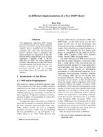
Abstract— Implementation of a new modular AC-AC matrix
converter and its control system are described. The converter
consists of a matrix connection of capacitor-clamped H-bridge
switch cells. The AC output of each switch cell can assume three
voltage levels during conduction. Input and output three-phase
AC waveforms are synthesized from pulse-width modulation of
the DC clamp capacitor voltages.
The space-vector modulation approach can be adapted to
control this converter. A control algorithm is described that can
be reduced to an equivalent DC-link converter. This controller
is implemented using programmable logic devices and a flash-
memory look-up table. Operational waveforms are presented.
I. INTRODUCTION
Multilevel conversion has attracted significant attention, as a
way to construct a relatively high-power converter using many
relatively-small power-semiconductor devices [1–3]. This ap-
proach has the advantages of reduced switching loss and
reduced harmonic content of output AC waveforms. The peak
voltages applied to the semiconductor devices are clamped to
capacitors whose DC voltages can be controlled via feedback,
and total switching loss is reduced. When the input and output
voltage magnitudes differ significantly, it is also possible to
reduce the conduction losses using multilevel techniques; this

property can improve the energy capture of variable-speed
wind power systems. Although multilevel conversion requires
a larger packaging and parts count, the total silicon area can
in principle be reduced because of the reduced device voltage
ratings. Thus, higher performance is attained at the expense
of increased control and complexity.
As the number of levels is increased, the bus bar structures
of multilevel DC-link converter systems can become quite
complex and difficult to fabricate. Several authors have sug-
gested a solution to this problem through the use of voltage-
clamped switch cells [4,5], in which the voltages applied to the
semiconductor devices are locally clamped to voltage sources.
The difficulty with this approach is that the voltage sources
of each switch cell must generate the average power supplied
by the inverter, and hence floating sources of DC power are
required.
To address these issues, a new family of modular matrix
converters was proposed in [6]. Voltage-clamped switch cells
This work was supported in part by the DOE National Renewable Energy
Laboratory under contract no. XCX-9-29204-01.
are connected in a matrix configuration as illustrated in Fig. 1.
Each switch cell consists of an H-bridge with a DC capacitor
whose voltage is controllable. The bus bar structures of this
modular approach are relatively easy to construct. The use
of a matrix configuration eliminates the need for DC voltage
sources that supply average power, and hence the voltage
sources are replaced by simple DC capacitors.
+

+


+

+

+

+

a
b
c
ABC
n
N
i
a
i
b
i
c
i
A
i
B
i
C
Three-phase
ac system 1
Three-phase

ac system 2
Fig. 1: New modular matrix converter.
Q
1
Q
2
Q
3
Q
4
D
1
D
2
D
3
D
4
Fig. 2: H-bridge switch cell with capacitor.
The new modular converter is fundamentally different from
the conventional matrix converter [7, 8], as well as from the
multilevel DC-link converter, in several respects. It is capable
of both increasing and decreasing the voltage magnitude and
frequency, while operating with arbitrary power factors. The
peak semiconductor device voltages are locally clamped to
a DC capacitor voltage, whose magnitude can be regulated.
The semiconductor devices are effectively utilized. Multilevel
switching can be used to synthesize the voltage waveforms
TABLE I: Comparison of conventional matrix converter with
new modular matrix converter.

Conventional matrix
converter
Proposed new modular
matrix converter
Voltage conversion
ratio V
out
/V
in
Buck:
V
out
≤ 0.866V
in
Buck-Boost:
0 ≤ V
out
< ∞
Switch
commutation
Coordination of 4-
quadrant switches
Simple transistor plus
freewheeling diode
Bus bar structure Complex Modular and simple
Multilevel operation No Possible
Filter elements AC capacitors and
inductors
Inductors
at both the input and output ports of the converter; switch

cells can be connected in series in each branch of the matrix
to increase the voltage rating of the converter. Switch com-
mutation is simpler than in the conventional matrix converter.
The new modular matrix converter and the conventional matrix
converter are compared in Table I.
The converter is capable of increasing the number of level of
operation by connecting more than one switch cell in series.
For example, when two switch cells are series-connected in
each branch as in Fig. 3. The converter can operate with three-
and four-level switching.
N
Three-phase
ac system 1
Three-phase
ac system 2
ABC
a
b
c
+

+

+

n
i
A
i
B

i
C
+

+

+

i
a
i
b
i
c
Fig. 3: Converter containing two switch cells in each branch
of the switch matrix.
This paper documents a laboratory prototype converter,
along with measured waveforms and data. A control algorithm
is described that is based on an equivalent DC-link converter.
Pulse-width modulated line-to-line voltages are synthesized by
switching the DC capacitor voltages of the switch cells. This
algorithm is implemented using programmable logic devices
and a flash-memory lookup table. The prototype switches at 50
kHz, using hard-switched 600 V IGBTs. The switch modules
are assembled on printed circuit boards.
II. PROPOSED CONTROL STRATEGY
A. Space Vector Modulation
The space vector modulation approach is a well-known
technique for control of three-phase converters [7]. This ap-
TABLE II: Nineteen combinations of line-to-line voltage, for

the basic converter configuration.
Three-phase variables D-Q variables
V
ab
V
bc
V
ca
V
d
V
q
V
cap
0 −V
cap
V
cap
√
3
3
V
cap
0 V
cap
−V
cap
0
2
√

3
3
V
cap
−V
cap
V
cap
0 −V
cap
√
3
3
V
cap
−V
cap
0 V
cap
−V
cap
−
√
3
3
V
cap
0 −V
cap
V

cap
0
2
√
3
3
V
cap
V
cap
−V
cap
0 V
cap
−
√
3
3
V
cap
2V
cap
−V
cap
−V
cap
2V
cap
0
V

cap
V
cap
−2V
cap
V
cap
√
3V
cap
−V
cap
2V
cap
−V
cap
−V
cap
√
3V
cap
−2V
cap
V
cap
V
cap
−2V
cap
0

−V
cap
−V
cap
2V
cap
−V
cap
−
√
3V
cap
V
cap
−2V
cap
V
cap
V
cap
−
√
3V
cap
2V
cap
0 −2V
cap
2V
cap

2
√
3
3
V
cap
0 2V
cap
−2V
cap
0
4
√
3
3
V
cap
−2V
cap
2V
cap
0 −2V
cap
2
√
3
3
V
cap
−2V

cap
0 2V
cap
−2V
cap
−
2
√
3
3
V
cap
0 −2V
cap
2V
cap
0
4
√
3
3
V
cap
2V
cap
−2V
cap
0 2V
cap
−

2
√
3
3
V
cap
00000
proach can be adapted for control of the proposed new modular
matrix converters. For the basic configuration of Fig. 1, the
instantaneous line-to-line voltages +2V
cap
, +V
cap
, 0, −V
cap
or −2V
cap
can be produced, where V
cap
is the DC capacitor
voltage of the switch cells. This leads to nineteen combinations
of valid balanced three-phase line-to-line voltages, as shown
in Table II. The line-to-line voltages are transformed into d-q
variables by the following equation.

v
d
(t)
v
q

(t)

=
2
3

cos(0) cos(120
◦
)cos(240
◦
)
sin(0) sin(120
◦
)sin(240
◦
)



v
x
(t)
v
y
(t)
v
z
(t)



(1)
q-axis
d-axis
(0,-4V
cap
/Ö3)
(0,4V
cap
/Ö3)
(0,2V
cap
/Ö3)
(0,-2V
cap
/Ö3)
(-V
cap
, -Ö3V
cap
)
(V
cap
, -Ö3V
cap
)
(V
cap
,Ö3V
cap
)

(-V
cap
, Ö3V
cap
)
(-2V
cap
, 2V
cap
/Ö3)
(-2V
cap
, -2V
cap
/Ö3)
(2V
cap
, -2V
cap
/Ö3)
(2V
cap
, 2V
cap
/Ö3)
(-2V
cap
, 0)
(2V
cap

, 0)
(V
cap
, V
cap
/Ö3)
(V
cap
, -V
cap
/Ö3)
(-V
cap
, -V
cap
/Ö3)
(-V
cap
, V
cap
/Ö3)
Fig. 4: Nineteen-space vector generated by proposed converter
Figure 4 shows the corresponding space vectors of all nine-
teen combinations in the d-q plane. These space vectors have
four different magnitudes: 0, 2V
cap
/
√
3, 2V
cap

and 4V
cap
/
√
3.
The inner ring of six low-magnitude vectors, the first group in
Table II, and the null space vector can be employed for two-
level switching. The outer ring of medium and high magnitude
vectors can be used for three-level switching; however, in the
basic converter configuration three-level switching is restricted
to voltage conversion ratios less than 57% or greater than
173%. This occurs because generation of a medium- or high-
magnitude space vector on one side of the converter forces
the other side to the null space vector [6]. Additional space
vectors are possible when multiple modules are placed in each
branch of the matrix.
f
V
k
V
l
v
ref
60
oV
0
d
k
V
k

d
l
V
l
Fig. 5: Space vector modulation.
The reference space vector can be expressed as a linear
combination of three adjacent space vectors, two low magni-
tude space vectors and the null space vector, as illustrated in
Fig. 5. It can also be described by the following equation:
v
ref
(t)=d
k
V
k
+ d
l
V
l
+ d
0
V
0
(2)
where d
k
, d
l
and d
0

are duty cycles of V
k
, V
l
and V
0
,
respectively, and
d
k
+ d
l
+ d
0
=1 (3)
By solving Eq. (2) and (3), we obtain
d
k
=
V
ref

V
k
sin60
◦
sinφ =
2
√
3

V
ref

V
k

sin φ
=
V
ref

V
cap
sin φ = M sin φ
d
l
=
V
ref

V
l
sin 60
◦
sin(60
◦
− φ)=
2
√
3

V
ref

V
l

sin(60
◦
− φ)
=
V
ref

V
cap
sin(60
◦
− φ)=M sin(60
◦
− φ)
d
0
=1− d
k
− d
l
=1− M sin(60
◦
+ φ)
M =

V
ref

V
cap
(4)
B. Single-Capacitor Control Scheme
When the converter synthesizes the input- and output-side
voltages, there exist additional degrees of freedom that can
be used to control the DC capacitor voltages. when the
converter operates with two-level switching, only one capacitor
is needed in each switching period. This approach is optimized
in sense of minimizing circulating current among capacitors.
An extra degree of freedom that can be used to control
the capacitor voltage is the pattern of space vectors in each
modulation period. To achieve the single-capacitor control
Input side
Output side
TS
d
0_in
max(d
k_in,
d
l_in
)
d
0_out
123 4 5
Subinterval

min(d
k_in,
d
l_in
)
max(d
m_out,
d
n_out
) min(d
m_out,
d
n_out
)
Fig. 6: The ordering pattern of input and output space vector
for two-level operation.
scheme, the pattern of Fig. 6 has been used. Consider the
case where the input reference space vector lies between
space vectors V
k in
and V
l in
, and the output reference space
vector lies between space vectors V
m out
and V
n out
. The
space vector modulation technique involves modulation among
input-side space vectors V

k in
, V
l in
and V
0 in
, with duty
cycles of d
k in
, d
l in
and d
0 in
respectively. Likewise, the
output-side involves modulation among output space vectors
V
m out
, V
n out
and V
0 out
with duty cycles of d
m out
, d
n out
and d
0 out
respectively. In each switching period, for both
the input- and output-sides, the pattern starts with the null
space vector then follows with the active space vector that
has maximum duty cycle, and then ends with the active space

vector that has less duty cycle. This space vector modulation
control requires that the switching period be divided into
five subintervals. For each combination of input space vector
and output space vector, different set of capacitors can be
employed. With the ordering pattern of input and output
space vector, as in Fig. 6, there exists one capacitor that can
be employed to synthesize terminal voltages throughout the
switching period.
Consider the example in which the input reference space
vector lies between space vectors V
3 in
and V
4 in
and the
output reference space vector lies between space vectors
V
1 out
and V
6 out
, as shown in Fig. 7. The pattern of input
and output space vectors in one switching period is shown
in Fig. 8, and the sets of capacitors that can be employed
for each subinterval are also shown. Notice that capacitor
C
Aa
, from the switch cell that is connected between input
phase A and output phase a, can be employed throughout the
switching period. Figure 9(a) summarizes how the converter
Input-Side Space Vector Diagram
Input reference

voltage space vector
d-axis
q-axis
f
in
V
1
V
2
V
3
V
4
V
5
V
6
V
0
(-V
cap
, V
cap
/Ö3)
(-V
cap
, -V
cap
/Ö3)
Output-Side Space Vector Diagram

Output reference
voltage space vector
d-axis
q-axis
f
out
V
1
V
2
V
3
V
4
V
5
V
6
V
0
(V
cap
, V
cap
/Ö3)
(V
cap
, -V
cap
/Ö3)

Fig. 7: Control example, at an instant when the input and
output side reference space vectors lie as shown.
OUTPUT SIDEI
NPUT SIDE
-Vcap+
Phase A
Phase B
Phase C
Phase a
Phase b
Phase c
V
ab
= Vcap
V
bc
= 0V
V
ca
= -Vcap
V
AB
= -Vcap
V
BC
= 0V
V
CA
= Vcap
-Vcap+

Phase A
Phase B
Phase C
Phase a
Phase b
Phase c
V
ab
= Vcap
V
bc
= -Vcap
V
ca
= 0V
V
AB
= -Vcap
V
BC
= 0V
V
CA
= Vcap
-Vcap+
Phase A
Phase B
Phase C
Phase a
Phase b

Phase c
V
AB
= -Vcap
V
CA
= 0V
V
ab
= Vcap
V
ca
= 0V
V
bc
= -VcapV
BC
= Vcap
V
CA
= 0V
Phase A
Phase B
Phase C
Phase a
Phase b
Phase c
-Vcap+
V
AB

= 0V
V
ab
= Vcap
V
bc
= 0V
V
ca
= -Vcap
V
BC
= 0V
Branch Aa
V
CA
= 0V
Phase A
Phase B
Phase C
Phase a
Phase b
Phase c
V
AB
= 0V
V
ab
= 0V
V

bc
= 0V
V
ca
= 0V
V
BC
= 0V
Single capacitor control
+
-
a
b
c
A
B
C
+
-
a
b
c
A
B
C
+
-
a
b
c

A
B
C
+
-
a
b
c
A
B
C
+
-
a
b
c
A
B
C
Equivalent DC link
01 46
v
AB
v
BC
v
CA
v
ab
v

bc
v
ca
0
0
0
0
0
0
 V
cap
 V
cap
 V
cap
+ V
cap
+ V
cap
+ V
cap
t
T
s
00 41 36
Line-to-line voltages
(a) (b) (c)
Fig. 9: Single capacitor control technique (a) switch combinations of each subinterval, (b) equivalent DC-link circuit, (c) the
resulting input and output waveforms.
Input side

Output side
T
S
Input V
0_in
d
0
T
s
Input V
4_in
Input V
3_in
d
4
T
s
d
3
T
s
Output V
0_out
Output V
1_out
Output V
6_out
d
0
T

s
d
1
T
s
d
6
T
s
12345
Subinterval
Possible
capacitors
that can be
used
C
Aa
C
Ba
C
Ca
C
Aa
C
Bb
C
Bc
C
Cb
C

Cc
C
Aa
C
Ac
C
Bb
C
Cb
C
Aa
C
Ac
C
Bb
C
Ca
C
Cc
Fig. 8: Ordering pattern of input and output space vectors
with switch cell capacitors that can be used in each
subinterval.
is configured for each subinterval. Figure 9(b) illustrates the
connections in an equivalent DC link converter that generates
identical space vectors. The instantaneous input and output
line-to-line voltages for both converters are illustrated in
Fig. 9(c).
Selection of the switch-cell capacitor to be employed during
a given switching period is based on the directions of the
reference space vectors, as well as relative values of the

duty cycles for the input- and output-side null space vectors.
Figure 10 summaries the result, for the case d
0 out
<d
0 in
.
A different switch-cell capacitor is selected for every 60
◦
of
the output-side line cycle, and for every 120
◦
of the input-side
line cycle. The situation is reversed when d
0 out
>d
0 in
.It
should be noted that, when the reference vector coincides with
V
1
V
2
V
3
V
4
V
5
V
6

C
_a
C
_c
C
_a
C
_b
C
_c
C
_b
C
Ca
C
Ba
C
Aa
C
Cb
C
Bb
C
Ab
C
Cc
C
Bc
C
Ac

C
Cc
C
Ac
C
Bc
C
Ca
C
Aa
C
Ba
C
Cb
C
Ab
C
Bb
Fig. 10: Summary of switch-cell capacitor choice, for the case
of d
0 out
<d
0 in
. The large (outer) space vector dia-
gram represents the output side, with 60
◦
segments.
When the 60
◦
segment is shaded, then the positive

side of V
cap
is applied to the respective output termi-
nal. The smaller superimposed space vector diagrams
represent the input side, with 120
◦
segments. The
case d
0 out
>d
0 in
is symmetrical, with the input
and output sides interchanged.
one of the converter space vectors V
1
, V
2
, , V
6
, then the
corresponding line-to-neutral voltage v
an
, −v
cn
, v
bn
, −v
an
,
v

cn
, −v
bn
, attain their peak values. Thus the single-capacitor
control scheme employs the capacitor from the switch cell that
is connected between the input phase and output phase that
have the largest opposite polarity line-to-neutral voltages.
For example, suppose that d
0 out
is less than d
0 in
.If
v
ref−out
(t) lies within ±30
◦
of the converter space vector
V
3
, and hence the output-side line-to-neutral voltage v
bn
(t)
is within ±30
◦
of its peak positive value for the output AC
line cycle. Therefore we choose one of the three capacitors
connected to the output phase b: either C
Ab
, C
Bb

or C
Cb
.
Next, the input side is examined. To narrow the choice to a
single capacitor, we select the phase having the largest negative
value, of opposite polarity to output side. Three of the six
converter space vectors lead to a negative-polarity input space
vector: V
2
, V
4
and V
6
correspond to negative v
CN
, v
AN
and v
BN
, respectively. The converter space vector that lies
closest to (within ± 60
◦
) of the input reference space vector is
selected. For instance, if the input-side reference space vector
lies between converter space vectors V
4
and V
5
, then it is
closest to converter negative space vector V

4
, and so input
phase A exhibits the most negative line-to-neutral voltage.
Therefore, capacitor C
Ab
is employed.
C. Eight-Capacitor Control Scheme
For comparison, the eight-capacitor control scheme is also
described. In this control scheme, all nine branches conduct
currents at any given time and capacitors are allowed to be
Phase A
Phase B
Phase C
Phase a
Phase b
Phase c
V
AB
= -Vcap
V
CA
= 0V
V
ab
= Vcap
V
ca
= 0V
V
bc

= -Vcap
V
BC
= Vcap
-Vcap+
-Vcap+
-V
c
a
p
+
+Vcap-
-Vcap+
Phase A
Phase B
Phase C
Phase a
Phase b
Phase c
V
CA
= 0V
V
ab
= Vcap
V
ca
= -Vcap
V
bc

= 0 V
V
BC
= 0 V
-Vcap+
-Vcap+
-Vcap+
V
AB
= 0 V
Phase A
Phase B
Phase C
Phase a
Phase b
Phase c
V
AB
= 0V
V
CA
= 0V
V
ab
= 0V
V
ca
= 0V
V
bc

= 0V
V
BC
= 0V
Phase A
Phase B
Phase C
Phase a
Phase b
Phase c
V
AB
= -Vcap
V
CA
= Vcap
V
ab
= Vcap
V
ca
= -Vcap
V
bc
= 0V
V
BC
= 0V
-Vcap+
+Vcap-

+Vcap-
+Vcap-
+Vcap-
Phase A
Phase B
Phase C
Phase a
Phase b
Phase c
V
AB
= -Vcap
V
CA
= Vcap
V
ab
= Vcap
V
ca
= 0V
V
bc
= -Vcap
V
BC
= 0V
-Vcap+
-V
c

a
p
+
+Vcap-
+Vcap-
Fig. 11: Configuration that used multiple capacitor connected
in parallel.
connected in parallel during each subinterval of Fig. 6. The
redundant switch combinations are employed in such a way
that the number of conducting capacitors is maximized. In
one switching period, the converter employs eight of nine
capacitors (three, four or five capacitors are employed in
each subinterval). This modulation scheme is related to the
single-capacitor control scheme of Figs. 8 and 9 in that
the subintervals, space vectors, and instantaneous line-to-line
voltage waveforms, are identical. The voltages across the
nonconducting branches of Fig. 9(a) are determined; those
branches blocking zero volts are switched to the shorting state,
while those branches that block voltage ±V
cap
are turned on
with their capacitors connected with the correct polarity. The
switching pattern of Fig. 11 is obtained. Close examination
of Fig. 11 reveals that the capacitor of branch Ab is never
employed. With this modulation approach, exactly eight of the
nine capacitors participates during each complete switching
period.
To the extent that the capacitor voltages remain balanced,
this scheme can improve efficiency by distributing the currents
over all nine branches. It also has the advantage that the

effective capacitance is increased, and hence capacitor voltage
ripple is reduced, and also that the capacitor voltage control
is reduced to a single control loop. The disadvantage is
that high peak currents can occur if the capacitor voltages
are unbalanced. Efficient operation of this scheme requires
that the mechanisms that drive capacitor voltage imbalances
(primarily from the energy stored in stray inductances of the
interconnections between switch cells) be minimized.
III. IMPLEMENTATION
A block diagram of the control system is shown in Fig. 12.
The input and output voltages and currents are sensed by
Hall effect devices, and are digitized using analog-to-digital
converters (ADC). The microcontroller transforms these into
d-q coordinates, as in Eq. (1). The DC capacitor voltages
of the nine switch cells are also measured using differential
amplifier circuits, and digitized using ADC’s. The microcon-
troller performs the space vector modulation, Eq. (4), and
chooses the capacitor for the single-capacitor control scheme.
The microcontroller is interfaced to the switch cells through
complex programmable logic devices (CPLDs). The CPLDs
are addressable by the microcontroller, and store the current
states of all switches. In addition, the states of all switches
during the next sub-interval can be loaded into the CPLDs.
The CPLDs implement the functions of timing and pulse-width
modulation.
The capacitor and space vector data are decoded by lookup
table to generate the state of each switch cell. These data
are further decoded by other CPLDs into the gate signals for
the IGBTs. To avoid cross-conduction of the IGBTs during
their switching transitions, which would lead to momentary

shorting of the DC bus voltages through the IGBTs, the turn-
off transitions of the IGBTs occurs first. In other words,
those IGBTs that were previously on, but will be turned
off, are switched first. After a controllable delay, the turn-on
transitions are triggered (i.e., the IGBTs that were previously
Turn on
Turn off
Voltage and
current sense
circuits
Code
representing
present
interval
Load values
of space
vectors for
each of 5
intervals
Capacitor #
Load values
of four duty
cycles per sw
period
19 bit data bus
representing present input
and output space vectors
and capacitor #
Lookup table
(Flash memory)

Converters space vectors
to switch states
Lookup table
(Flash memory)
Converters space vectors
to switch states
Lookup table
(Flash memory)
Converters space vectors
to switch states
Switch cell control
(CPLD)
Switch cell control
(CPLD)
Switch cell control
(CPLD)
Data buffer
(CPLD)
Clock
25 MHz
Delay Delay
To opto-isolated
gate driver
Phase A
To opto-isolated
gate driver
Phase B
To opto-isolated
gate driver
Phase C

Compensates for
latency of flash
memory
Sets dead time to ensure non-overlapping
conduction
Delays implemented within timer CPLD
Decoding logic
Break before make
logic
Alternating
conduction logic
High-level control
algorithm
Space-vector control of
converter currents
Field-oriented control of
generator
}
}
40 MHz
Microproceesor
A/C
Converters
update data
every 100 msec
Timer (CPLD)
40 ns resolution
for each interval
Fig. 12: Block diagram of the control system.
off, but will be turned on, are switched). The gate signals from

the CPLDs are sent through opto-isolated gate driver circuits
to the IGBTs in power stage.
IV. EXPERIMENTAL RESULTS
A prototype was constructed to demonstrate the validity
of the control strategy. The prototype was connected to the
60 Hz utility, and transferred power to resistive load. The
input line-to-line voltages are sensed and used as the reference
input space vector. The output space vector was programmed
in the microcontroller. The converter operated at a switching
frequency of 50 kHz.
Figures 13 to 15 show the waveforms for operation with
the single-capacitor control scheme. The converter was pro-
grammed to produce an output frequency of 30 Hz, with
Fig. 13: Input and output waveforms for the single-capacitor
control scheme. Trace 1: 60 Hz line-to-line voltage
at input terminal. Trace 2: 60 Hz input current. Trace
3: 30 Hz line-to-line output voltage. Trace 4: 30 Hz
output current.
Fig. 14: Waveforms from single-capacitor control scheme: ca-
pacitor voltage and 30 Hz output voltage
Fig. 15: Waveforms from single-capacitor control scheme: ca-
pacitor voltage and filtered 30 Hz output voltage.
Fig. 16: Input and output waveforms for the eight-capacitor
control scheme. Trace 1: 60 Hz line-to-line voltage
at input terminal. Trace 2: 60 Hz input current. Trace
3: 30 Hz line-to-line output voltage. Trace 4: 30 Hz
output current.
Fig. 17: Waveforms from multiple-capacitor control scheme:
capacitor voltage and 30 Hz output voltage
Fig. 18: Waveforms from multiple-capacitor control scheme:

capacitor voltage and filtered 30 Hz output voltage.
input modulation index, M
in
= V
ref−in
/V
cap
, of 0.94
and output modulation index, M
out
= V
ref−out
/V
cap
,
of 0.87. Figures 16 to 18 show the waveforms when the
converter operated with the eight-capacitor control scheme.
The converter was also programmed to produce the same
operating point as in the single-capacitor control scheme case.
V. CONCLUSION
The laboratory experiment proves that the proposed new
modular matrix converter is valid and operates as claimed.
Space vector control of both the input and output side has
been implemented, to convert a given three-phase input into
a three-phase output of given desired frequency, magnitude,
and phase. With both the single-capacitor control scheme and
the multiple-capacitor control scheme, it was observed that the
capacitor voltages naturally remained balanced and stable. The
converter operated with an IGBT switching frequency of 50
kHz.

R
EFERENCES
[1] A. Nabae, I. Takahashi, and H. Akagi, “A New Neutral-Point Clamped
PWM Inverter,” IEEE Trans. on Industry Applications, vol. IA-17,
pp. 518–523, Sep./Oct. 1981.
[2] P. Bhagwat and V. Stefanovi´c, “Generalized Structure of a Multilevel
PWM Inverter,” IEEE Trans. on Industry Applications, vol. IA-19,
pp. 1057–1069, Nov./Dec. 1983.
[3] L. M. Tolbert and F. Z. Peng, “Multilevel Converter for Large Electric
Drives,” IEEE Applied Power Electronics Conference, vol. 2, pp. 530–
536, 1998.
[4] B. Lin, Y. Chien, and H. Lu, “Multilevel Inverter with Series Connection
of H-Bridge Cells,” IEEE International Conference on Power Electronics
and Drive Systems, pp. 859–864, Jul. 1999.
[5] F. Z. Peng, J. S. Lai, J. McKeever, and J. VanCoevering, “A Multilevel
Voltage-Source Inverter with Separate DC Sources for Static VAR Gen-
eration,” Conf. Rec. of IEEE IAS Annual Meeting, vol. 3, pp. 2541–2548,
Oct. 1995.
[6] R. W. Erickson and O. A. Al-Naseem, “A New Family of Matrix Convert-
ers,” IEEE Industrial Electronics Society Annual Conference (IECON’01),
vol. 2, pp. 1515–1520, Nov./Dec. 2001.
[7] L. Huber and D. Borojevi´c, “Space Vector Modulation Three-Phase to
Three-Phase Matrix Converter with Input Power Factor Correction,” IEEE
Trans. on Industry Applications, vol. 31, Nov./Dec. 1995.
[8] J. Oyama, T. Higuchi, E. Yamada, T. Koga, and T. Lipo, “New Con-
trol strategy for Matrix Converter,” IEEE Power Electronics Specialists
Conference, pp. 360–367, 1989.