Problems – Chapter 1
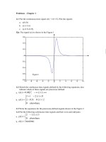
1.1 Plot the continuous-time signal x(t) = t/(1+t
4
). Plot the signals:
a. x(0.5t)
b. x(-t+3.6)
c. x(-0.7t-0.35)
Tip: The signal x(t) is shown in the Figure 1
-10 -8 -6 -4 -2 0 2 4 6 8 10
-0.8
-0.6
-0.4
-0.2
0
0.2
0.4
0.6
1.2 Sketch the continuous-time signals defined by the following equations; also
indicate which of these signals are piecewise defined
a.
+∞≤≤∞−= tt08.0)t(x
3
b.





<≤−
<≤−+
=

elsewhere0
2t0t5.02
0t2t2
)t(y
1.3 Write the equations for the piecewise-defined signals shown in the Figure 2
1.4 Plot the following continuous-time signals and their even and odd parts.
a.



≤≤−
=
elsewhere0
3t12
)t(y
b.
)t6sin(3)t(z π=
Figure1
1.5 The block diagrams for the feedback control system are shown in Figure 3. Write
the system equation for it.
1.6 Draw block-diagram representations for the systems characterized by the
following system equations, where x(t) is the input and y(t) is the output.
a)
)t(x3
dt
)t(dx
)t(y2
dt
)t(dy
5 +=+

b)
dt
)t(dx
2)t(xd)(y8.0)t(y5.0
t
+=ττ+
∫
∞−
1.7 Determine whether the systems having the following system equations are linear,
whether the systems are time-invariant. State the reasons for your answers.
a)
dt
)t(dy
)t(x3)t(y
2
+=
b)
dt
)t(dx
)t(tx4)t(y
dt
)t(yd
2
2
−+=
10
20
-12 -8 -4 0 4 8 12
3
6

-0.3 -0.2 -0.1 0 0.1 0.2 0.3
0.312
Figure 2
x(t)
y(t)
3
∫
∞−
t
2
∫
∞−
t
0.5 d/dt
Figure 3
Problems – Chapter 2
2.1 Find the time delay of the following sinusoidal functions with respect to the
reference cosine function.
a)
)2.1t4000cos(20)t(v +π=
b)
)11.0t120cos(8)t(i −π=
2.2 For the circuit node shown in the Figure 1, find i
4
(t) when i
1
(t) = 3cos(40t-0.1),
i
2
(t) = 5cos(40t+0.2), and i

3
(t) = 3cos(40t-2)
2.3 The RC circuit shown in Figure 2 designed to high-frequency interference that
occurs along with a lower frequency telemetry signal at the input. Find the output
signal y(t) when the input signal is x(t) = x
l
(t) + x
h
(t), where
)25.0t2cos(10)t(x
l
−=
is
the telemetry signal and
)5.0t150cos(8.0)t(x
h
−=
is the interference signal.
Does the filter circuit perform the function it was designed to perform?
2.4 Plot the following signals:
a) x(t) = 2r(t+2)-2r(t+1)-2r(t)+2r(t-1)
b) y(t) = 2+r(t-2)-r(t-4)
c)
)4t(u4)t2(u2
2
3t
)t(r)t(g −+−+







−
Π=
2.5 Write the equation for the test signal shown in the Figure 3 in terms of a sum of
step and/or ramp functions.
i
4
(t)
i
3
(t)
i
2
(t)
i
1
(t)
Figure 1
Ω
40
y(t)
x(t)
2 mF
Figure 2
2
1
-3 -2 -1 0 1 2 3
Figure 3

2.6 The input and output signals of the filter circuit in Figure 4 are the voltages x(t)
and y(t), respectively
a) Find the system equation for the circuit
b) Find y(t) for t >= 0 when x(t) = t for t >= 0, y(0) = ½ volt, and i(0) = 1/3 ampere
2.7 A second-order system is represented by the block diagram shown in Figure 5.
a) Find the system equation for the system
b) Solve the system equation to find y(t) for t >= 0 when x(t) = 2e
-3t
for t >= 0, y(0) =
1 and y’(0) = -1.
2.8 Compute the convolution of the two continuous frequency functions
fallfor)f5.0sin(3)f(y
4|f|0
4|f|1
)f(x
π=



>
≤
=
2.9 Find and sketch the convolution of the functons shown in the Figure 6.
∩∩∩
Ω
2/5
x(t)
1/3 F
y(t)
1/2 H

Figure 4
-2 -1 0 1 2
-2 -1 0 1 2
Figure 6
x(t)
y(t)
∫
t
0
3
Figure 5
2/3
∫
t
0
2.10 Prove that the convolution is commutative, associativity and distributive
Problems _ Chapter 3
3.1 Plot the single-sided and double-sided amplitude and phase spectra for the
following signals:
a)
)5.0t1000cos(6)t(x −π=
b)
)2.0t6cos(3)t2sin(10)t(v +π−π=
c)
)t6cos(2)2.1t5.1cos()4.6t5.4sin(4)t(y π++π−π=
3.2
a) Find the complex-exponential Fourier series representation for the signal
t1)t(x −=
over the interval
1t0 ≤≤

b) Find the complex-exponential Fourier series representation for the signal



<−
≥−
=
0tt
0tt1
)t(y
over the interval
1|t| <
3.3 Given the periodic signal






−
Π=
−=
−
∞
−∞=
∑
20
5t
e)t(x
where

)i20t(x)t(x
t1.0
p
i
p
Find the single-sided amplitude and phase spectra and the double-sided amplitude and
phase spectra of x(t). Plot the spectra for
Hz3.0f ≤
3.4 The signal x(t) has a spectrum
fj2
3
)f(X
π+
=
Use the theorems to find the spectrum for the following signals
a)
dt
)t(dx
2)t(x
a
=
b)
)t2(x)t(x
b
−−=
c)
)4/t(x)t(x
c
−=
d)

t6cos)t(x3)t(x
d
π=
e)
)3t4(x)t(x
e
−=
3.5 Use the table of Fourier transforms and the theorems to find the spectra for the
signals shown in Figure 1.
3.6 A system has the frequency response
f45j)f500(
500
)f(H
2
+−
=
and an input
signal
)4/t80cos()3/t20cos()t10cos()t(x π−π+π+π+π=
a) Find and plot the system amplitude and phase response
b) Find and plot the amplitude and phase spectra for the input and output signals.
3.7 Plot the amplitude and phase responses, and approximate the system half-power
bandwidth and half-power cutoff frequencyfor the system with the frequency response
below
H(f) = 100/(50 + jf)
3.8 A system is characterized by the system differential equation
)t(x
dt
)t(dx
)t(y5.0

dt
)t(dy
+=+
a) Find the system frequency response
b) Plot the system amplitude and phase response
c) Find the system impulse response
t (s)
2
1
0 2 4
t (s)
-2 0 2
1
x(t)
y(t)
Figure 1
Problems _ Chapter 4
4.1 Find the double-sided Laplace transforms and convergence regions for
)t(ue)t(yand)t(ue)t(x
atat
−−==
−−
(Hint: the transforms are the same but the convergence regions are different)
4.2 Use tables and theorems to find the Laplace transforms of the following signals:
a)
)3t(u3)t(u3)t(x −−=
b)
)2t(u)1t(r)t(r)t(y −−−−=
c)
)t(ue10)t(u10)t(w

t−
−=
d)
)t(u)t4cos(3)t(z =
4.3 Use tables and theorems to find the Laplace transforms of the following signals:
a)
)3t(r)1t(r2)t(u)1t()t(x −+−−+=
b)
)1t(u)e1()t(y
t
−−=
−
c)
)t(u)t2cos()t2sin(10)t(w =
d)
)]2t(u)t(u[t)t(z −−=
e)
)t(u)]t2cos(2ee[)t(h
t5t
−+=
−
4.4 Find the inverse laplace transforms of
a)
)3s)(2s(s
1s
)s(X
++
+
=
b)

21s10s
s
)s(Y
2
++
=
c)
16s12s2
2s4
)s(W
2
++
+
=
4.5 Find the inverse Laplace transforms of
a)
3
2
)1s)(2s(
8s16s2
)s(X
++
+−
=
b)
)25s6s)(1s(
42s24s2
)s(Y
2
2

++−
++−
=
c)
s16s
e448s20s5
)s(H
3
s22
+
−+−
=
−
4.6 Use Laplace transforms to solve the following differential equation for y(t) for t
>= 0, subject to the given initial conditions.
3
dt
)0(dy
;2)0(y
)t(u8)t(y10
dt
)t(dy
7
dt
)t(yd
2
−==
=++
−
−

4.7 A feedback control system for a manufacturing process is represented by the
transformed block diagram shown in Figure 1, where X(s) and Y(s) are the the
transforms of the input and output signals, respectively.
a) Find the system transfer function
b) Find the system response y(t), for K = 0 and for K = 0.125 when the input signal
x(t) is a unit step
4.8 Determine whether the systems defined by the following transfer functions are
stable, marginally stable or unstable
a)
2ss
1
)s(H
2
−+
=
b)
)4s)(1s(
3s
)s(H
++
−
=
c)
5s2s
s
)s(H
2
+−
=
d)

3ss
2s
)s(H
2
++
+
=
4.9 A system has the transformed block diagram shown in Figure 2, where X(s) and
Y(s) are the the transforms of the input and output signals, respectively.
a) Find the system transfer function
b) Draw the system pole-zero plot
c) Find the system impulse
response
X(s) Y(s)
H
2
(s) = K
Figure 1
)1s(s
10
)s(H
1
+
=
Y(s)
X(s)
3/s
6s+160
)2s(s
1

+
Figure 2
Problems _ Chapter 5
5.1 Consider a random process given by
)tf2cos(A)t(X
0
φ+π=
, where A and f
0

are constants and
φ
is a random variable that is uniformly distributed over
)2,0( π
. If
X(t) is an ergodic process, the time averages of X(t) in the limit as
∞→t
are equal
to corresponding ensemble averages of X(t).
a) Use time averaging over an integer number of periods to calculate the
approximations to the first and second moments of X(t)
b) Use the equations of mean value and mean-square value of X to calculate the
ensemble-average approximations to the first and second moments of X(t)
c) Compare the results between part (a) and part (b), and give your comment.
5.2 Figure 2 illustrates an M-level linear quantizer for an analog signal. The analog
waveform m(t) is approximated with the quantized waveform m
q
(t). This
approximation will result in the quantization error. The step size between quantization
levels, called the quantile interval, is denoted S.

Assume that the quantization error is uniformly distributed over a single quantile
interval S-wide, calculate the quantization error variance.
m
-2
m
-1
m
0
S/2
S
m
q
(t)
m(t)
m
1
m
2
Figure 2
Problems _ Chapter 6
6.1
a) Define the ideal high-pass filter. Sketch the amplitude and phase responses
b) Write the mathematical expression for the frequency response of the ideal high-
pass filter. Find the impulse response
6.2
a) Define the ideal band-stop filter. Sketch the amplitude and phase responses
b) Write the mathematical expression for the frequency response of the ideal band-
stop filter. Find the impulse response
6.3 Find the transfer functions for the minimum-phase, stable filters with the
amplitude responses:

a)
42
2
56
)16(2
|)j(H|
ω+ω+
ω+
=ω
b)
42
42
4174
64684
|)j(H|
ω+ω+
ω+ω+
=ω
6.4 Find the transfer functions for the minimum-phase, stable filters with the
amplitude responses:
a)
42
42
4265576
64.020100
|)j(H|
ω+ω+
ω+ω+
=ω
b)

42
42
22018
5.01032
|)j(H|
ω+ω+
ω+ω+
=ω
6.5 The maximum gain of a low pass filter is to be 0.8. The gain is to vary no more
than 3 dB from 0 to 5 kHz and is to be less than or equal to one-tenth of the maximum
gain for
kHz10f ≥
. Determine the mimimum order of Buterworth filter that will
meet the specifications.
6.6 Find the transfer function for a Butterworth band pass filter that has two poles, a
center frequency of 500 Hz, a bandwidth of 100 Hz, and a maximum gain of unity.
6.7 A band stop filter is needed to reduce power source hum (60 Hz) in an amplifier.
It is constructed by transforming a normalized Buterworth low pass filter. The
resulting filter is to have unity maximum gain and a stop band with lower and upper
cutoff frequencies of 50 and 70 Hz, respectively. The gain between 57 and 61 Hz is to
be less than or equal to 0.04. Find the transfer function.
/>%22Compute+the+convolution+of+the+two+continuous+frequency+functions
%22&source=web&ots=yvqSJu5Tbl&sig=hmNOim3SsUY8APUeqVGmD1RfIoQ&
hl=vi&sa=X&oi=book_result&resnum=1&ct=result#PPA27,M1