- Trang chủ >>
- Khoa Học Tự Nhiên >>
- Vật lý
liboff r. kinetic theory.. classical, quantum, and relativistic descriptions
Bạn đang xem bản rút gọn của tài liệu. Xem và tải ngay bản đầy đủ của tài liệu tại đây (2.43 MB, 592 trang )
Kinetic Theory:
Classical, Quantum, and
Relativistic Descriptions,
Third Edition
Richard L. Liboff
Springer
Graduate Texts in Contemporary Physics
Series Editors:
R. Stephen Berry
Joseph L. Birman
Mark P. Silverman
H. Eugene Stanley
Mikhail Voloshin
Springer
New York
Ber lin
Heidelberg
Hong Kong
London
Milan
Paris
Tokyo
This page intentionally left blank
Richard L. Liboff
Kinetic Theory
Classical, Quantum,
and Relativistic Descriptions
Third Edition
With 112 Illustrations
13
Richard L. Liboff
School of Electrical Engineering
Cornell University
Ithaca, NY 14853
Series Editors
R. Stephen Berry Joseph L. Birman Mark P. Silverman
Department of Chemistry Department of Physics Department of Physics
University of Chicago City College of CUNY Trinity College
Chicago, IL 60637 New York, NY 10031 Hartford, CT 06106
USA USA USA
H. Eugene Stanley Mikhail Voloshin
Center For Polymer Studies Theoretical Physics Institute
Physics Department Tate Laboratory of Physics 424
Boston University The University of Minnesota
Boston, MA 02215 Minneapolis, MN 55455
USA USA
Library of Congress Cataloging-in-Publication Data
Liboff, Richard L., 1931–
Kinetic theory: classical, quantum, and relativistic descriptions / Richard L. Liboff
3rd ed.
p. cm.—(Graduate texts in contemporary physics)
Includes bibliographical references and index.
ISBN 0-387-95551-8 (alk. paper)
1. Kinetic theory of matter. I. Title. II. Series.
QC174.9 L54 2003
530.13
6—dc21 2002026658
ISBN 0-387-95551-8 Printed on acid-free paper.
The second edition of this book was published © 1998 by John Wiley & Sons.
© 2003 Springer-Verlag New York, Inc.
All rights reserved. This work may not be translated or copied in whole or in part without the written
permission of the publisher (Springer-Verlag New York, Inc., 175 Fifth Avenue, New York, NY 10010,
USA), except for brief excerpts in connection with reviews or scholarly analysis. Use in connection
with any form of information storage and retrieval, electronic adaptation, computer software, or by
similar or dissimilar methodology now known or hereafter developed is forbidden.
The use in this publication of trade names, trademarks, service marks, and similar terms, even if they
are not identified as such, is not to be taken as an expression of opinion as to whether or not they are
subject to proprietary rights.
Printed in the United States of America.
987654321 SPIN 10887268
www.springer-ny.com
Springer-Verlag New York Berlin Heidelberg
A member of BertelsmannSpringer Science+Business Media GmbH
To the Memory of
Harold Grad
Teacher and Friend
This page intentionally left blank
I learned much from my teachers, more
from my colleagues and most of all from
my students
Rabbi Judah ha-Nasi (ca. 135–C.E.)
Babylonian Talmud (Makkot, 10a)
Ludwig Boltzmann (University of Vienna, courtesy AIP Emilio Segr
`
e Visual
Archives)
Preface to the Third Edition
Since the first edition of this work, kinetic theory has maintained its position as
a cornerstone of a numberofdisciplines in science and mathematics. In physics,
such is the case for quantum and relativistic kinetic theory. Quantum kinetic
theory finds application in the transport of particles and radiation through
material media, as well as the non-stationary quantum–many-body problem.
Relativistic kinetic theory is relevant to controlled thermonuclear fusion and to
a number of problems in astrophysics. In applied mathematics, kinetic theory
relates to the phenomena of localization, percolation, and hopping, relevant to
transport properties in porous media. Classical kinetic theory is the foundation
of fluid dynamics and thus is important to aerospace, mechanical, and chemical
engineering. Important to the study of transport in metals is the Lorentz–
Legendre expansion, which in this new edition appears in an appendix. A new
section in Chapter 1 was included in this new edition that addresses constants of
motion and symmetry. A number of small but important revisions were likewise
made in this new edition. A more complete description of the contents of the
text follows.
The text comprises seven chapters. In Chapter 1, the transformation theory
of classical mechanics is developed for the purpose of deriving Liouville’s the-
orem and the Liouville equation. Four distinct interpretations of the solution
to this equation are presented. The fourth interpretation addresses Gibbs’s no-
tion of a distribution function that is the connecting link between the Liouville
equation and experimental observation. The notion of a Markov process is
discussed, and the central-limit theorem is derived and applied to the random
walk problem.
In Chapter 2, the very significant BBKGY hierarchy is obtained from the
Liouville equation, and the first two equations of this sequence are applied in
the derivation of conservation of energy for a gas of interacting particles. In
x Preface to the Third Edition
nondimensionalizing this sequence, parameters emerge that differentiate be-
tween weakly and strongly coupled fluids. Correlation functions are introduced
through the Mayer expansions. Examining a weakly coupled fluid composed
of particles interacting under long-range interaction leads to the Vlasov equa-
tion and the closely allied concept of a self-consistent solution. Prigogine’s
diagrammatic technique and related operator formalism for examining the
Liouville equation are described. The Bogoliubov ansatz concerning the equi-
libration of a gas, as well as the Klimontovich formulation of kinetic theory,
are also included in this chapter.
The Boltzmann equation is derived in Chapter 3 and applied to the derivation
of fluid dynamic equations and the H theorem. Poincar
´
e’s recurrence theorem
is proved and is discussed relative to Boltzmann’s H theorem. Transport coeffi-
cients are defined, and the Chapman–Enskog expansion is developed. Results
of this technique of solution to the Boltzmann equation are compared with
experimental data and are found to be in good agreement for various molec-
ular samples. Grad’s method of solution of the Boltzmann equation involving
expansion in tensor Hermite polynomials is described. The chapter continues
with a derivation of the Druyvesteyn distribution relevant to a current carrying
plasma in a dc electric field. In the last section of the chapter, the topic of irre-
versibility is revisited. Ergodic and mixing flows are discussed. Action-angle
variables are introduced, and the notions of classical degeneracy and resonant
domains in phase space are described in relation to the chaotic behavior of
classical systems. A statement of the closely allied KAM theorem is also given.
In the first half of Chapter 4, the Vlasov equation is applied to linear
wave theory for a two-component plasma composed of electrons and heavy
ions. Landau damping and the Nyquist criterion for wave instabilities are
described. The chapter continues with derivations of other important ki-
netic equations: Krook–Bhatnager–Gross (KBG),Fokker–Planck, Landau,and
Balescu–Lenard equations. A table is included describing the interrelation of
the classical kinetic equations discussed in the text. The chapter concludes with
a description of the widely used Monte Carlo numerical analysis in kinetic
theory.
Quantum kinetic theory is developed in Chapter 5. A brief review of ba-
sic principles leads to a description of the density matrix, the Pauli equation,
and the closely related Wigner distribution. Various equivalent forms of the
Wigner–Moyal equation are derived. A quantum modified KBG equation is
applied to photon transport and electron propagation in solids. Thomas–Fermi
screening and the Mott transition are also discussed. The Uehling–Uhlenbeck
quantum modified Boltzmann equation is developed and applied to a Fermi
liquid. The chapter continues with an overview of classical and quantum hier-
archies of equations connecting reduced distributions. A table of hierarchies
is included where the reader is easily able to view distinctions among these
sets of equations. The Kubo formula, described previously in Chapter 3, is
revisited and applied to the derivation of a quantum expression for electrical
Preface to the Third Edition xi
conductivity. The chapter concludes with an introduction to Green’s function
analysis and related diagrammatic representations.
Chapter 6 addresses relativistic kinetic theory. The discussion begins with el-
ementary concepts, including a statement of Hamilton’s equations in covariant
form. Stemming from a covariant distribution function in four space, together
with Maxwell’s equations in covariant form, a relativistic Vlasov equation
is derived for a plasma in an electromagnetic field. An important compo-
nent of this chapter is the derivation and compilation of a table of Lorentz
invariants in kinetic theory. The chapter continues with a derivation of the
relativistic Maxwellian and concludes with a brief description of relativity in
non-Cartesian coordinates.
Chapter 7 has been added in this new edition, and addresses kinetic and
thermal properties of metals and amorphous media. The first component
of the chapter begins with a review of the notion of thermopower, and the
Wiedermann–Franz law is derived. The discussion continues with a formula-
tion for electrical and thermal conductivity in metals (encountered previously
in Chapter 5), stemming from the quantum Boltzmann equation, in which
Bloch’s classic low-temperature T
5
dependence of metallic resistivity and
canonical high-temperature linear T dependence are derived. In addition, the
formalism yields a residual resistivity at 0 K. The chapter continues with a
discussion of properties of amorphous media and related processes of local-
ization, hopping, and percolation. Bloch waves and the notion of extended
states are reviewed. Anderson’s parameter of the ratio of the spread-of-states
to the band width is introduced. Localization occurs at some critical value of
this parameter. At smaller values of the parameter, energies of localized and
extended states are separated at the “mobility edge.” Transition of the Fermi
energy from the domain of extended states to the domain of localized states
represents the Mott metal–insulator transition. Mechanisms of electrical con-
duction are discussed in three temperature intervals in which the notions of
thermally assisted and variable-range hopping emerge. The chapter continues
with the concepts of bond and site percolation. A number of percolation scal-
ing laws are discussed. The chapter concludes with a review of localization
in second quantization. Throughout the chapter, many discussions related to
material science are included.
Each chapter is preceded by a brief introductory statement of the subject
matter contained in the chapter. Problems appear at the end of each chapter,
many of which carry solutions. A number of problems include self-contained
descriptions of closely allied topics. In such cases, these are listed in the chapter
table of contents under the heading, Topical Problems. In addition to references
cited in the text, a comprehensive list of references is included in Appendix E.
Assorted mathematical formulas are included in Appendices A and B, includ-
ing a list of properties of Laguerre and Hermite polynomials (B4). Appendix
D, addressing the Lorentz–Legendre expansion in kinetic theory, is new to this
edition.
xii Preface to the Third Edition
Stemming from the observation that science and society are inextricably
entwined, a time chart is included (Appendix E) listing early contributors to
science and technology of the classical Greek and Roman eras. The reader will
note that a central figure in this display is the Greek philosopher, Democritus,
who, at about 400 BCE, was the first to propose an atomic theory of matter.
Readers of my earlier work [Introduction to the Theory of Kinetic Equations,
Wiley, New York (1969)] will recall that it, too, included a time chart describing
contributions to dynamics from the fifteenth to the nineteenth centuries. The
appendix on Mathematical Formulas has been expanded in this new edition to
include a list of properties of Laguene and Hermite polynomials (Appendix
B4).
Many individuals have contributed to the development of this work. I remain
indebted to these kind colleagues and would like here to express my sincere
gratitude for their encouragement, support, and constructive criticism: Sidney
Leibovich, Terrence Fine, Robert Pay, Christof Litwin, Kenneth Gardner, Neal
Maresca, K. C. Liu, Danny Heffernan, Edwin Dorchek, Philip Bagwell, Ronald
Kline, Steve Seidman, S. Ramakrishna, G. George, Timir Datta, William Mor-
rell, Wayne Scales, Daniel Koury, Erich Kunhardt, Marvin Silver, Hercules
Neves, James Hartle, Kenneth Andrews, Clifford Pollock, VeitElser, Chuntong
Ying, Michael Parker, Jack Freed, Richard Zallen, Abner Shimony, Philip
Holmes, Lloyd Hillman, Arthur Ruoff, L. Pearce Williams, Lloyd Motz, John
Guckenheimer, Isaac Rabinowitz, Gregory Schenter, and Ilya Prigogine.
Some of these individuals are former students. It is due to my association
with these gifted and talented colleagues that the talmudic inscription for this
work is motivated.
Peace,
Richard L. Liboff
Contents
Preface to the Third Edition ix
1 The Liouville Equation 1
1.1 Elements of Classical Mechanics 2
1.1.1 Generalized Coordinates and the Lagrangian . . . 2
1.1.2 Hamilton’s Equations 4
1.1.3 Constants of the Motion 6
1.1.4 -Space 7
1.1.5 Dynamic Reversibility 9
1.1.6 Equation of Motion for Dynamical Variables . . . 10
1.2 Canonical Transformations 11
1.2.1 Generating Functions 11
1.2.2 Generating Other Transformations 14
1.2.3 Canonical Invariants 15
1.2.4 Group Property of Canonical Transformations . . 15
1.2.5 Constants of Motion and Symmetry 16
1.3 Liouville Theorem 17
1.3.1 Proof 17
1.3.2 Geometric Significance 18
1.3.3 Action Generates the Motion 19
1.4 Liouville Equation 20
1.4.1 The Ensemble: Density in Phase Space 20
1.4.2 First Interpretation of D(q,p,t) 20
1.4.3 Most General Solution: Second Interpretation of
D(q,p,t) 22
1.4.4 Incompressible Ensemble 23
1.4.5 Method of Characteristics 24
xiv Contents
1.4.6 Solutions to the Initial-Value Problem 25
1.4.7 Liouville Operator 27
1.5 Eigenfunction Expansions and the Resolvent 29
1.5.1 Liouville Equation Integrating Factor 29
1.5.2 Example: The Ideal Gas 30
1.5.3 Free-Particle Propagator 32
1.5.4 The Resolvent 33
1.6 Distribution Functions 35
1.6.1 Third Interpretation of D(q,p,t) 35
1.6.2 Joint-Probability Distribution 36
1.6.3 Reduced Distributions 37
1.6.4 Conditional Distribution 37
1.6.5 s-Tuple Distribution 38
1.6.6 Symmetric Properties of Distributions 39
1.7 Markov Process 41
1.7.1 Two-Time Distributions 41
1.7.2 Chapman–Kolmogorov Equation 41
1.7.3 Homogeneous Processes in Time 43
1.7.4 Master Equation 43
1.7.5 Application to Random Walk 44
1.8 Central-Limit Theorem 47
1.8.1 Random Variables and the Characteristic Function 47
1.8.2 Expectation, Variance, and the Characteristic
Function 47
1.8.3 Sums of Random Variables 49
1.8.4 Application to Random Walk 50
1.8.5 Large n Limit: Central-Limit Theorem 54
1.8.6 Random Walk in Large n Limit 55
1.8.7 Poisson and Gaussian Distributions 57
1.8.8 Covariance and Autocorrelation Function 59
Problems 60
2 Analyses of the Liouville Equation 77
2.1 BBKGY Hierarchy 78
2.1.1 Liouville, Kinetic Energy, and Remainder
Operators 78
2.1.2 Reduction of the Liouville Equation 80
2.1.3 Further Symmetry Reductions 81
2.1.4 Conservation of Energy from BY
1
and BY
2
83
2.2 Correlation Expansions: The Vlasov Limit 86
2.2.1 Nondimensionalization 86
2.2.2 Correlation Functions 89
2.2.3 The Vlasov Limit 90
2.2.4 The Vlasov Equation: Self-Consistent Solution . 92
2.2.5 Debye Distance and the Vlasov Limit 95
Contents xv
2.2.6 Radial Distribution Function 96
2.3 Diagrams: Prigogine Analysis 97
2.3.1 Perturbation Liouville Operator 98
2.3.2 Generalized Fourier Series 99
2.3.3 Interpretation of a
l
Coefficients 99
2.3.4 Equations of Motion for a
(k)
Coefficients 102
2.3.5 Selection Rules for Matrix Elements 103
2.3.6 Properties of Diagrams 104
2.3.7 Long-Time Diagrams: The Boltzmann Equation . 107
2.3.8 Reduction of Time Integrals 108
2.3.9 Application of Diagrams to Plasmas 113
2.4 Bogoliubov Hypothesis 115
2.4.1 Time and Length Intervals 115
2.4.2 The Three Temporal Stages 115
2.4.3 Bogoliubov Distributions 117
2.4.4 Density Expansion 117
2.4.5 Construction of F
(0)
2
119
2.4.6 Derivation of the Boltzmann Equation 121
2.5 Klimontovich Picture 124
2.5.1 Phase Densities 124
2.5.2 Phase Density Averages 125
2.5.3 Relation to Correlation Functions 126
2.5.4 Equation of Motion 127
2.6 Grad’s Analysis 127
2.6.1 Liouville Equation Revisited 127
2.6.2 Truncated Distributions 128
2.6.3 Grad’s First and Second Equations 129
2.6.4 The Boltzmann Equation 130
Problems 132
3 The Boltzmann Equation, Fluid Dynamics, and Irreversibility 137
3.1 Scattering Concepts 138
3.1.1 Separation of the Hamiltonian 138
3.1.2 Scattering Angle 140
3.1.3 Cross Section 143
3.1.4 Kinematics 146
3.2 The Boltzmann Equation 149
3.2.1 Collisional Parameters and Derivation 149
3.2.2 Multicomponent Gas 153
3.2.3 Representation of Collision Integral for Rigid
Spheres 153
3.3 Fluid Dynamic Equations and the Boltzmann H Theorem 155
3.3.1 Collisional Invariants 155
3.3.2 Macroscopic Variables and Conservative Equations 157
xvi Contents
3.3.3 Conservation Equations and the Boltzmann
Equation 159
3.3.4 Temperance: Variance of the Velocity Distribution 161
3.3.5 Irreversibility 162
3.3.6 Poincar
´
e Recurrence Theorem 163
3.3.7 Boltzmann and Gibbs Entropies 164
3.3.8 Boltzmann’s H Theorem 166
3.3.9 Statistical Balance 167
3.3.10 The Maxwellian 168
3.3.11 The Barometer Formula 170
3.3.12 Central-Limit Theorem Revisited 172
3.4 Transport Coefficients 174
3.4.1 Response to Gradient Perturbations 174
3.4.2 Elementary Mean-Free-Path Estimates 178
3.4.3 Diffusion and Random Walk 186
3.4.4 Autocorrelation Functions, Transport Coefficients,
and Kubo Formula 188
3.5 The Chapman–Enskog Expansion 194
3.5.1 Collision Frequency 194
3.5.2 The Expansion 195
3.5.3 Second-Order Solution 199
3.5.4 Thermal Conductivity and Stress Tensor 202
3.5.5 Sonine Polynomials 203
3.5.6 Application to Rigid Spheres 207
3.5.7 Diffusion and Electrical Conductivity 208
3.5.8 Expressions of
(l,q)
for Inverse Power Interaction
Forces 209
3.5.9 Interaction Models and Experimental Values . . . 211
3.5.10 The Method of Moments 213
3.6 The Linear Boltzmann Collision Operator 217
3.6.1 Symmetry of the Kernel 217
3.6.2 Negative Eigenvalues 218
3.6.3 Comparison of Boltzmann and Liouville Operators 219
3.6.4 Hard and Soft Potentials 220
3.6.5 Maxwell Molecule Spectrum 220
3.6.6 Further Spectral Properties 222
3.7 The Druyvesteyn Distribution 225
3.7.1 Basic Parameters and Starting Equations 225
3.7.2 Legendre Polynomial Expansion 227
3.7.3 Reduction of
ˆ
J
0
(f
0
| F) 232
3.7.4 Evaluation of I
0
and I
1
Integrals 233
3.7.5 Druyvesteyn Equation 236
3.7.6 Normalization, Velocity Shift, and Electrical
Conductivity 237
Contents xvii
3.8 Further Remarks on Irreversibility 240
3.8.1 Ergodic Flow 240
3.8.2 Mixing Flow and Coarse Graining 243
3.8.3 Action-Angle Variables 245
3.8.4 Hamilton–Jacobi Equation 248
3.8.5 Conditionally Periodic Motion and Classical
Degeneracy 249
3.8.6 Bruns’s Theorem 253
3.8.7 Anharmonic Oscillator 253
3.8.8 Resonant Domains and the KAM Theorem 255
Problems 258
4 Assorted Kinetic Equations with Applications to Plasmas and
Neutral Fluids 278
4.1 Application of the Vlasov Equation to a Plasma 279
4.1.1 Debye Potential and Dielectric Constant 279
4.1.2 Waves, Instabilities, and Damping 285
4.1.3 Landau Damping 288
4.1.4 Nyquist Criterion 292
4.2 Further Kinetic Equations of Plasmas and Neutral Fluids . 294
4.2.1 Krook–Bhatnager–Gross Equation 295
4.2.2 KBG Analysis of Shock Waves 298
4.2.3 The Fokker–Planck Equation 301
4.2.4 The Landau Equation 307
4.2.5 The Balescu–Lenard Equation 309
4.2.6 Convergent Kinetic Equation 315
4.2.7 Fokker–Planck Equation Revisited 317
4.3 Monte Carlo Analysis in Kinetic Theory 319
4.3.1 Master Equation 319
4.3.2 Equivalence of Master and Integral Equations . . 320
4.3.3 Interpretation of Terms 321
4.3.4 Application of Random Numbers 323
4.3.5 Program for Evaluation of Distribution Function . 324
Problems 325
5 Elements of Quantum Kinetic Theory 329
5.1 Basic Principles 330
5.1.1 The Wave Function and Its Properties 330
5.1.2 Commutators and Measurement 332
5.1.3 Representations 334
5.1.4 Coordinate and Momentum Representations . . . 335
5.1.5 Superposition Principle 337
5.1.6 Statistics and the Pauli Principle 339
5.1.7 Heisenberg Picture 339
5.2 The Density Matrix 341
xviii Contents
5.2.1 The Density Operator 342
5.2.2 The Pauli Equation 346
5.2.3 The Wigner Distribution 351
5.2.4 Weyl Correspondence 354
5.2.5 Wigner–Moyal Equation 357
5.2.6 Homogeneous Limit: Pauli Equation Revisited . . 359
5.3 Application of the KBG Equation to Quantum Systems . 363
5.3.1 Equilibrium Distributions 363
5.3.2 Photon Kinetic Equation 366
5.3.3 Electron Transport in Metals 369
5.3.4 Thomas–Fermi Screening 376
5.3.5 Mott Transition 378
5.3.6 Relaxation Time for Charge-Carrier Phonon
Interaction 379
5.4 Quantum Modifications of the Boltzmann Equation . . . 385
5.4.1 Quasi-Classical Boltzmann Equation 385
5.4.2 Kinetic Theory for Excitations in a Fermi Liquid 387
5.4.3 H Theorem for Quasi-Classical Distribution . . . 392
5.5 Overview of Classical and Quantum Hierarchies 394
5.5.1 Second Quantization and Fock Space 394
5.5.2 Classical and Quantum Distribution Functions . . 395
5.5.3 Equations of Motion 399
5.5.4 Generalized Hierarchies 400
5.6 Kubo Formula Revisited 403
5.6.1 Charge Density and Current 403
5.6.2 Identifications for Kubo Formula 404
5.6.3 Electrical Conductivity 405
5.6.4 Reduction to Drude Conductivity 407
5.7 Elements of the Green’s Function Formalism 408
5.7.1 Schr
¨
odinger Equation Green’s Function 408
5.7.2 The s-Body Green’s Function 410
5.7.3 Averages and the Green’s Function 410
5.7.4 The Quasi-Free Particle 413
5.7.5 One-Body Green’s Function 414
5.7.6 Retarded and Advanced Green’s Functions 415
5.7.7 Coupled Green’s Function Equations 415
5.7.8 Diagrams and Expansion Techniques 416
5.8 Spectral Function for Electron–Phonon Interactions . . . 421
5.8.1 Hamiltonian 421
5.8.2 Green’s Function Equations of Motion 423
5.8.3 The Spectral Function 425
5.8.4 Lorentzian Form 426
5.8.5 Lifetime and Energy of a Quasi-Free Particle . . 428
Problems 429
Contents xix
6 Relativistic Kinetic Theory 449
6.1 Preliminaries 450
6.1.1 Postulates 450
6.1.2 Events, World Lines, and the Light Cone 450
6.1.3 Four-Vectors 451
6.1.4 Lorentz Transformation 452
6.1.5 Length Contraction, Time Dilation, and Proper
Time 454
6.1.6 Covariance, Hamiltonian, and Hamilton’s
Equations 454
6.1.7 Criterion for Relativistic Analysis 455
6.2 Covariant Kinetic Formulation 456
6.2.1 Distribution Function 456
6.2.2 One-Particle Liouville Equation 457
6.2.3 Covariant Electrodynamics 458
6.2.4 Vlasov Equation 459
6.2.5 Covariant Drude Formulation of Ohm’s Law . . . 460
6.2.6 Lorentz Invariants in Kinetic Theory 461
6.2.7 Relativistic Electron Gas and Darwin Lagrangian 464
6.3 The Relativistic Maxwellian 467
6.3.1 Normalization 467
6.3.2 The Nonrelativistic Domain 469
6.4 Non-Cartesian Coordinates 470
6.4.1 Covariant and Contravariant Vectors 470
6.4.2 Metric Tensor 471
6.4.3 Lagrange’s Equations 472
6.4.4 The Christoffel Symbol 473
6.4.5 Liouville Equation 474
Problems 474
7 Kinetic Properties of Metals and Amorphous Media 480
7.1 Metallic Electrical and Thermal Conduction 482
7.1.1 Background 482
7.1.2 Thermopower 484
7.1.3 Electron–Phonon Scattering Matrix Elements . . 487
7.1.4 Quantum Boltzmann Equation 493
7.1.5 Perturbation Distribution 496
7.1.6 Electrical Resistivity 498
7.1.7 Scale Parameters of ρ
0
503
7.1.8 Electron Distribution Function 504
7.1.9 Thermal Conductivity 504
7.2 Amorphous Media 505
7.2.1 Background 505
7.2.2 Localization 508
7.2.3 Conduction Mechanisms and Hopping 511
xx Contents
7.2.4 Percolation Phenomena 514
7.2.5 Pair-Connectedness Function and Scaling 517
7.2.6 Localization in Second Quantization 520
Problems 524
Location of Key Equations 527
List of Symbols 529
Appendices
A Vector Formulas and Tensor Notation 537
A.1 Definitions 537
A.2 Vector Formulas and Tensor Equivalents 539
B Mathematical Formulas 541
B.1 Tensor Integrals and Unit Vector Products 541
B.2 Exponential Integral, Function, ζ Function, and Error
Function 542
B.2.1 Exponential Integral 542
B.3 Other Useful Integrals 545
B.4 Hermite and Laguerre Polynomials and the Hypergeometric
Function 546
C Physical Constants 550
D Lorentz–Legendre Expansion 552
E Additional References 554
E.1 Early Works 554
E.2 Recent Contributions to Kinetic Theory and Allied Topics 558
F Science and Society in the Classical Greek and Roman Eras 563
Index 565
CHAPTER 1
The Liouville Equation
Introduction
This chapter begins with a review of the basic principles and equations of
classical mechanics. These lead naturally to the Liouville theorem, which to-
gether with the notions of ensemble and phase space, give rise to the Liouville
equation. This equation is perhaps the most significant relation in all of clas-
sical kinetic theory, and in the remainder of the chapter various techniques
of solution to this equation, as well as various interpretations of its solution,
are presented. Thus, for example, it is found that the Liouville equation is an
equation of motion for the N-particle joint-probability distribution, where N
denotes the number of particles in the system. Integration of this distribution
over subdomains in phase space gives reduced distributions whose equations
of motion (BBKGY Eqs.) are developed in Chapter 2.
A discussion is included of the Chapman–Kolmogorov equation and the
closely allied master equation, which is applied to the random-walk problem.
The master equation emerges again in Chapter 5 in analysis of the quantum
mechanical density matrix.
The chapter concludes with a brief description of probability theory and a
derivation of the central-limit theorem. This theorem is applied to obtain the
long-time displacement of the random walk and yields the Gaussian distribu-
tion. This distribution is fundamental to diffusion theory and is encountered
again in Chapter 3. The central-limit theorem is likewise again encountered in
Chapter 3 in a derivation of the distribution of center-of-mass momenta of a
stationary gas of molecules. The discrete Poisson distribution is obtained from
random-walk results and applied to small shot noise.
2 1. The Liouville Equation
Classical mechanics and probability theory are the foundations of kinetic
theory. Consequently, a firm grasp of the basic principles and relations of these
formalisms will lead to a richer working knowledge of kinetic theory.
1.1 Elements of Classical Mechanics
1.1.1 Generalized Coordinates and the Lagrangian
The number of degrees of freedom a given system has is equal to the min-
imum number of independent parameters necessary to uniquely determine
the location and orientation of the system in physical space. Such indepen-
dent parameters are called generalized coordinates. Thus, for example, a rigid
dumbbell molecule free to move in three-space has five degrees of freedom:
three to locate the center of mass of the molecule and two (angles) to determine
the orientation of the molecule. A fluid of N such molecules has 5N degrees
of freedom. A rigid triangular molecule has six degrees of freedom: five to
locate an edge of the triangle and an additional angle to fix the orientation of
the plane of the molecule about this axis.
For a system with N degrees of freedom, generalized coordinates are labeled
q
1
, q
2
, , q
N
. These parameters may be taken to comprise the components
of an N-dimensional vector,
q (q
1
,q
2
, ,q
N
) (1.1)
The corresponding generalized velocities also comprise components of an
N-dimensional vector, and we write
˙q ( ˙q
1
, ˙q
2
, , ˙q
N
) (1.2)
The composite vector (q, ˙q) determines the state of the system.
Let the system at hand exist in a conservative force field with kinetic energy
T (q, ˙q) and potential V (q). The Lagrangian of the system is then given by
L(q, ˙q) T (q, ˙q) −V (q) (1.3)
The dynamics of the system may be formulated in terms of Hamilton’s prin-
ciple. This principle states that the motion of the system between two fixed
points, (q,t)
1
and (q,t)
2
, renders the action integral:
S
2
1
L(q, ˙q,t) dt (1.4)
an extremum.
1
That is,
δ
2
1
L(q, ˙q,t) dt 0 (1.5)
1
More precisely, a minimum.
1.1 Elements of Classical Mechanics 3
FIGURE 1.1. End points q
1
and q
2
are held fixed in the variation (1.5).
where δ denotes a variation about the motion of the system.
2
See Fig. 1.1
Lagrange’s equations
The dynamical principle (1.5) may be employed to obtain a differential
equation for L(q, ˙q,t). That is, let q(t) be the motion that renders S an
extremum.
Effecting the variation (1.5) and Taylor-series expanding the integrand gives
δS
2
1
L(q +δq, ˙q +δ ˙q, t) dt −
2
1
L(q, ˙q,t) dt
2
1
L +
δL
δq
· δq +
δL
δ ˙q
· δ ˙q
dt −
2
1
L(q, ˙q,t) dt (1.6)
Note that
∂L
∂ ˙q
d
dt
(δq)
d
dt
∂L
∂ ˙q
· δq)
−
d
dt
∂L
∂ ˙q
· δq
Inserting this expression into the preceding equation gives
∂L
∂ ˙q
· δq
2
1
+
2
1
∂L
∂q
−
d
dt
∂L
∂ ˙q
· δq dt 0
Since the end points of the trajectory are held fixed in the variation, the first
bracketed “surface terms” vanish. Insofar as the remaining integral must vanish
for any arbitrary, infinitesimal variation δq, it is necessary that
d
dt
∂L
∂ ˙q
l
−
∂L
∂q
l
0(l 1, 2, ,N) (1.7)
2
Furthermore, the variation is a virtual displacement, that is, on that occurs in
zero time.
4 1. The Liouville Equation
Here we have returned to the component representation of (q.˙q). Equa-
tions (1.7) are called Lagrange’s equations.
1.1.2 Hamilton’s Equations
When written in the form
d
dt
∂L
∂ ˙q
l
∂L
∂q
l
(1.8)
Lagrange’s equations (1.7) reveal the following important observation: If the
coordinate q
l
is missing in the Lagrangian, the quantity ∂L/∂ ˙q
l
is constant in
time. In this event, we say that the coordinate q
1
is cyclic or ignorable.
To better exhibit this symmetry principle of mechanics, we effect the
following transformation:
(q
l
, ˙q
l
) → (q
l
,p
l
) (1.9)
where
p
l
≡
∂L
∂ ˙q
l
(1.10)
The variable p
l
, so defined, is called the canonical momentum or momentum
conjugate to the coordinate q
l
.
The transformation (1.9) is accomplished through a Legendre transforma-
tion (familiar to thermodynamics). This transformation carries the Lagrangian
L(q, ˙q)totheHamiltonian H (q,p) by the following recipe:
H
l
∂L
∂ ˙q
l
˙q
l
− L (1.11)
Equations of motion in terms of the Hamiltonian are obtained by forming
the differential of the latter equation.
dH(q, p,t)
l
d
∂L
∂ ˙q
l
˙q
l
+
∂L
∂ ˙q
l
d ˙q
l
−
∂L
∂ ˙q
l
d ˙q
l
−
∂L
∂q
l
dq
l
−
∂L
∂t
dt
With Lagrange’s equations (1.7) and the definition (1.10), we obtain
dH(q, p,t)
l
( ˙q
l
dp
l
−˙p
l
dq
l
) −
∂L
∂t
dt
Expanding the left side of this equation and identifying terms gives
˙p
l
−
∂H
∂q
l
, ˙q
l
∂H
∂p
l
(1.12)
together with ∂H /∂t −∂L/∂t. Equations (1.12) are called Hamilton’s
equations.