located hidden random fields- learning discriminative parts for object detection
Bạn đang xem bản rút gọn của tài liệu. Xem và tải ngay bản đầy đủ của tài liệu tại đây (931.24 KB, 14 trang )
Located Hidden Random Fields: Learning
Discriminative Parts for Object Detection
Ashish Kapoor
1
and John Winn
2
1
MIT Media Laboratory, Cambridge, MA 02139, USA
2
Microsoft Research, Cambridge, UK
Abstract. This paper introduces the Located Hidden Random Field
(LHRF), a conditional model for simultaneous part-based detection and
segmentation of objects of a given class. Given a training set of images
with segmentation masks for the object of interest, the LHRF automati-
cally learns a set of parts that are both discriminative in terms of appear-
ance and informative about the location of the object. By introducing
the global position of the object as a latent variable, the LHRF models
the long-range spatial configuration of these parts, as well as their local
interactions. Experiments on benchmark datasets show that the use of
discriminative parts leads to state-of-the-art detection and segmentation
performance, with the additional benefit of obtaining a labeling of the
object’s component parts.
1 Introduction
This paper addresses the problem of simultaneous detection and segmentation
of objects belonging to a particular class. Our approach is to use a conditional
model which is capable of learning discriminative parts of an object. A part is
considered discriminative if it can be reliably detected by its local appearance
in the image and if it is well localized on the object and hence informative as to
the object’s location.
The use of parts has several advantages. First, there are local spatial inter-
actions between parts that can help with detection, for example, we expect to
find the nose right above the mouth on a face. Hence, we can exploit local part
interactions to exclude invalid hypotheses at a local level. Second, knowing the
location of one part highly constrains the locations of other parts. For example,
knowing the locations of wheels of a car constrains the positions where rest of
the car can be detected. Thus, we can improve object detection by incorporating
long range spatial constraints on the parts. Third, by inferring a part labeling
for the training data, we can accurately assess the variability in the appearance
of each part, giving better part detection and hence better object detection. Fi-
nally, the use of parts gives the potential for detecting objects even if they are
partially occluded.
A. Leonardis, H. Bischof, and A. Pinz (Eds.): ECCV 2006, Part III, LNCS 3953, pp. 302–315, 2006.
c
Springer-Verlag Berlin Heidelberg 2006
Located Hidden Random Fields: Learning Discriminative Parts 303
One possibility for training a parts-based system is to use supervised training
with hand-labeled parts. The disadvantage of this approach is that it is very
expensive to get training data annotated for parts, plus it is unclear which parts
should be selected. Existing generative approaches try to address these problems
by clustering visually similar image patches to build a codebook in the hope that
clusters correspond to different parts of the object. However, this codebook has
to allow for all sources of variability in appearance – we provide a discriminative
alternative where irrelevant sources of variability do not need to be modeled.
This paper introduces Located Hidden Random Field, a novel extension to
the Conditional Random Field [1] that can learn parts discriminatively. We in-
troduce a latent part label for each pixel which is learned simultaneously with
model parameters, given the segmentation mask for the object. Further, the ob-
ject’s position is explicitly represented in the model, allowing long-range spatial
interactions between different object parts to be learned.
2 Related Work
There have been a number of parts-based approaches to segmentation or detec-
tion. It is possible to pre-select which parts are used as in [2] – however, this re-
quires significant human effort for each new object class. Alternatively, parts can
be learned by clustering visually similar image patches [3, 4] but this approach
does not exploit the spatial layout of the parts in the training images. There
has been work with generative models that do learn spatially coherent parts in
an unsupervised manner. For example, the constellation models of Fergus et al.
[5,6] learn parts which occur in a particular spatial arrangement. However, the
parts correspond to sparsely detected interest points and so parts are limited in
size, cannot represent untextured regions and do not provide a segmentation of
the image. More recently, Winn and Jojic [7] used a dense generative model to
learn a partitioning of the object into parts, along with an unsupervised segmen-
tation of the object. Their method does not learn a model of object appearance
(only of object shape) and so cannot be used for object detection in cluttered
images.
As well as unsupervised methods, there are a range of supervised methods
for segmentation and detection. Ullman and Borenstein [8] use a fragment-based
method for segmentation, but do not provide detection results. Shotton et al. [9]
use a boosting method based on image contours for detection, but this does not
lead to a segmentation. There are a number of methods using Conditional Ran-
dom Fields (CRFs) to achieve segmentation [10] or sparse part-based detection
[11]. The OBJ CUT work of Kumar et al. [12] uses a discriminative model for
detection and a separate generative model for segmentation but requires that the
parts are learned in advance from video. Unlike the work presented in this paper,
none of these approaches achieves part-learning, segmentation and detection in
a single probabilistic framework.
Our choice of model has been motivated by Szummer’s [13] Hidden Random
Field (HRF) for classifying handwritten ink. The HRF automatically learns parts
304 A. Kapoor and J. Winn
of diagram elements (boxes, arrows etc.) and models the local interaction be-
tween them. However, the parts learned using an HRF are not spatially localized
as the relative location of the part on the object is not modeled. In this paper
we introduce the Located HRF, which models the spatial organization of parts
and hence learns part which are spatially localized.
3 Discriminative Models for Object Detection
Our aim is to take an n × m image x and infer a label for each pixel indicating
the class of object that pixel belongs to. We denote the set of all image pixels as
V and for each pixel i ∈ V define a label y
i
∈{0, 1} where the background class
is indicated by y
i
= 0 and the foreground by y
i
= 1. The simplest approach is to
classify each pixel independently of other pixels based upon some local features,
corresponding to the graphical model of Fig. 1a. However, as we would like to
model the dependencies between pixels, a conditional random field can be used.
Conditional Random Field (CRF): this consists of a network of classifiers
that interact with one another such that the decision of each classifier is influ-
enced by the decision of its neighbors. In the graphical model for a CRF, the class
label corresponding to every pixel is connected to its neighbors in a 4-connected
grid, as shown in Fig. 1b. We denote this new set of edges as E.
Givenanimagex, a CRF induces a conditional probability distribution
p(y |x, θ) using the potential functions ψ
1
i
and ψ
2
ij
. Here, ψ
1
i
encodes compatibil-
ity of the label given to the ith pixel with the observed image x and ψ
2
ij
encodes
(a)
Unary Classification
y
x
(b) CRF
y
x
(c) HRF
y
h
x
(d)
h
x
y
T
l
LHRF
Fig. 1. Graphical models for different discriminative models of images. The
image x and the shaded vertices are observed during training time. The parts h, denoted
by unfilled circles, are not observed and are learnt during the training. In the LHRF
model, the node corresponding to T is connected to all the locations l
i
,depictedusing
thick dotted lines.
Located Hidden Random Fields: Learning Discriminative Parts 305
the pairwise label compatibilities for all (i, j) ∈ E conditioned on x.Thus,the
conditional distribution p(y |x) induced by a CRF can be written as:
p(y |x; θ)=
1
Z(θ, x)
i∈V
ψ
1
i
(y
i
, x; θ)
(i,j)∈E
ψ
2
ij
(y
i
,y
j
, x; θ)(1)
where the partition function Z(θ, x) depends upon the observed image x as well
as the parameters θ of the model. We assume that the potentials ψ
1
i
and ψ
2
ij
take the following form:
ψ
1
i
(y
i
, x; θ
1
)=exp[θ
1
(y
i
)
T
g
i
(x)]
ψ
2
ij
(y
i
,y
j
, x; θ
2
)=exp[θ
2
(y
i
,y
j
)
T
f
ij
(x)]
Here, g
i
: R
n×m
→R
d
is a function that computes a d-dimensional feature
vector at pixel i, given the image x. Similarly, the function f
ij
: R
n×m
→R
d
computes the d-dimensional feature vector for edge ij.
Hidden Random Field: a Hidden Random Field (HRF) [13] is an extension to
aCRFwhichintroducesanumberofparts for each object class. Each pixel has
an additional hidden variable h
i
∈{1 H} where H is the total number of parts
across all classes. These hidden variables represent the assignment of pixels to
parts and are not observed during training. Rather than modeling the interaction
between foreground and background labels, an HRF instead models the local
interaction between the parts. Fig. 1c shows the graphical model corresponding
to an HRF showing that the local dependencies captured are now between parts
rather than between class labels. There is also an additional edge from a part
label h
i
to the corresponding class label y
i
. Similar to [13], we assume that
every part is uniquely allocated to an object class and so parts are not shared.
Specifically, there is deterministic mapping from parts to object-class and we
can denote it using y(h
i
).
Similarly to the CRF, we can define a conditional model for the label image
y and part image h:
p(y, h|x; θ)=
1
Z(θ, x)
i∈V
ψ
1
i
(h
i
, x; θ
1
) φ(y
i
,h
i
)
(i,j)∈E
ψ
2
ij
(h
i
,h
j
, x; θ
2
)(2)
where the potentials are defined as:
ψ
1
i
(h
i
, x; θ
1
)=exp[θ
1
(h
i
)
T
g
i
(x)]
ψ
2
ij
(h
i
,h
j
, x; θ
2
)=exp[θ
2
(h
i
,h
j
)
T
f
ij
(x)]
φ(y
i
,h
i
)=δ(y(h
i
)=y
i
)
where δ is an indicator function. The hidden variables in the HRF can be used to
model parts and interaction between those parts, providing a more flexible model
whichinturncanimprovedetectionperformance. However, there is no guarantee
that the learnt parts are spatially localized. Also, as the model only contains
local connections, it does not exploit the long-range dependencies between all
the parts of the object.
306 A. Kapoor and J. Winn
3.1 Located Hidden Random Field
The Located Hidden Random Field (LHRF) is an extension to the HRF, where
the parts are used to infer not only the background/foreground labels but also
a position label in a coordinate system defined relative to the object. We aug-
ment the model to include the position of the object T , encoded as a discrete
latent variable indexing all possible locations. We assume a fixed object size so a
particular object position defines a rectangular reference frame enclosing the ob-
ject. This reference frame is coarsely discretized into bins, representing different
discrete locations within the reference frame. Fig. 2 shows an example image,
the object mask and the reference frame divided into bins (shown color-coded).
Image Object Mask
Location Map
(a) (b) (c)
Fig. 2. Instantiation of different nodes in an LHRF. (a) image x, (b) class labels
y showing ground truth segmentation (c) color-coded location map l. The darkest color
corresponds to the background.
We also introduce a set of location variables l
i
∈{0, , L},wherel
i
takes the
non-zero index of the corresponding bin, or 0 if the pixel lies outside the reference
frame. Given a location T the location labels are uniquely defined according to
the corresponding reference frame. Hence, when T is unobserved, the location
variables are all tied together via their connections to T . These connections
allow the long-range spatial dependencies between parts to be learned. As there
is only a single location variable T , this model makes the assumption that there
is a single object in the image (although it can be used recursively for detecting
multiple objects – see Section 4).
We define a conditional model for the label image y,thepositionT , the part
image h and the locations l as:
p(y, h, l,T|x; θ)=
i∈V
ψ
1
i
(h
i
, x; θ
1
) φ(y
i
,h
i
) ψ
3
(h
i
,l
i
; θ
3
) δ(l
i
=loc(i, T ))
×
(i,j)∈E
ψ
2
ij
(h
i
,h
j
, x; θ
2
) ×
1
Z(θ, x)
(3)
where the potentials ψ
1
,ψ
2
,φ aredefinedasintheHRF,andloc(i, T )isthe
location label of the ith pixel when the reference frame is in position T .The
potential encoding the compatibility between parts and locations is given by:
ψ
3
(h
i
,l
i
; θ
3
)=exp[θ
3
(h
i
,l
i
)] (4)
where θ
3
(h
i
,l
i
) is a look-up table with an entry for each part and location index.
Located Hidden Random Fields: Learning Discriminative Parts 307
Table 1. Comparison of Different Discriminative Models
Parts-Based Spatially Models Local Models Long
Informative Spatial Range Spatial
Parts Coherence Configuration
Unary Classifier No – No No
CRF No – Yes No
HRF Yes No Yes No
LHRF Yes Yes Yes Yes
In the LHRF, the parts need to be compatible with the location index as
well as the class label, which means that the part needs to be informative about
the spatial location of the object as well as its class. Hence, unlike the HRF, the
LHRF learns spatially coherent parts which occur in a consistent location on the
object. The spatial layout of these parts is captured in the parameter vector θ
3
,
which encodes where each part lies in the co-ordinate system of the object.
Table 1 gives a summary of the properties of the four discriminative models
which have been described in this section.
4 Inference and Learning
There are two key tasks that need to be solved when using the LHRF model:
learning the model parameters θ and inferring the labels for an input image x.
Inference: Given a novel image x and parameters θ, we can classify an i
th
pixel as background or foreground by first computing the marginal p(y
i
|x; θ)
and assigning the label that maximizes this marginal. The required marginal is
computed by marginalizing out the part variables h, the location variables l,the
position variable T and all the labels y except y
i
.
p(y
i
|x; θ)=
y/y
i
h,l,T
p(y, h, l,T|x; θ)
If the graph had small tree width, this marginalization could be performed ex-
actly using the junction tree algorithm. However, even ignoring the long range
connections to T , the tree width of a grid is the length of its shortest side and
so exact inference is computationally prohibitive. The earlier described models,
CRF and HRF, all have such a grid-like structure, which is of the same size as
the input image; thus, we resort to approximate inference techniques. In par-
ticular, we considered both loopy belief propagation (LBP) and sequential tree-
reweighted message passing (TRWS) [14]. Specifically, we compared the accuracy
of max-product and the sum-product variants of LBP and the max-product form
of TRWS (an efficient implementation of sum-product TRWS was not available
– we intend to develop one for future work). The max-product algorithms have
the advantage that we can exploit distance transforms [15] to reduce the running
time of the algorithm to be linear in terms of number of states. We found that
308 A. Kapoor and J. Winn
both max-product algorithms performed best on the CRF with TRWS outper-
forming LBP. However, on the HRF and LHRF models, the sum-product LBP
gave significantly better performance than either max-product method. This is
probably because the max-product assumption that the posterior mass is con-
centrated at the mode is inaccurate due to the uncertainty in the latent part
variables. Hence, we used sum-product LBP for all LHRF experiments.
When applying LBP in the graph, we need to send messages from each h
i
to
T and update the approximate posterior p(T ) as the product of these; hence,
log p(T )=
i∈V
log
h
i
b(h
i
) ψ
3
(h
i
, loc(i, T )) (5)
where b(h
i
) is the product of messages into the ith node, excluding the message
from T . To speed up the computation of p(T ), we make the following approxi-
mation:
log p(T ) ≈
i∈V
h
i
b(h
i
)logψ
3
(h
i
, loc(i, T )). (6)
This posterior can now be computed very efficiently using convolutions.
Parameter Learning: Given an image x with labels y and location map l,
the parameters θ are learnt by maximizing the conditional likelihood p(y, l|x, θ)
multiplied by the Gaussian prior p(θ)=N(θ|0,σ
2
I). Hence, we seek to maximize
the objective function F(θ)=L(θ)+logp(θ), where L(θ) is the log of the
conditional likelihood.
F(θ)=logp(y, l|x;θ)+logp(θ)=log
h
p(y, h, l|x;θ)+logp(θ)
= −log Z(θ, x)+log
h
˜p(y, h, l, x; θ)+logp(θ)(7)
where:
˜p(y, h, l, x; θ)=
i
ψ
1
i
(h
i
, x; θ
1
)φ(y
i
,h
i
)ψ
3
(h
i
,l
i
; θ
3
)
(i,j)∈E
ψ
2
ij
(h
i
,h
j
, x; θ
2
).
We use gradient ascent to maximize the objective with respect to the para-
meters θ. The derivative of the log likelihood L(θ) with respect to the model
parameters θ = {θ
1
, θ
2
, θ
3
} can be written in terms of the features, single node
marginals and pairwise marginals:
δL(θ)
δθ
1
(h
)
=
i∈V
g
i
(x) ·(p(h
i
=h
|x, y, l; θ) −p(h
i
=h
|x; θ))
δL(θ)
δθ
2
(h
,h
)
=
(i,j)∈E
f
ij
(x) · (p(h
i
=h
,h
j
=h
|x, y, l; θ) −p(h
i
=h
,h
j
=h
|x; θ))
δL(θ)
δθ
3
(h
,l
)
=
i∈V
p(h
i
=h
,l
i
=l
|x, y, l; θ) −p(h
i
=h
,l
i
=l
|x; θ)
Located Hidden Random Fields: Learning Discriminative Parts 309
It is intractable to compute the partition function Z(θ, x) and hence the objec-
tive function (7) cannot be computed exactly. Instead, we use the approximation
to the partition function given by the LBP or TRWS inference algorithm, which
is also used to provide approximations to the marginals required to compute
the derivative of the objective. Notice that the location variable T comes into
effect only when computing marginals for the unclamped model (where y and l
are not observed), as the sum over l should be restricted to those configurations
consistent with a value of T. We have trained the model both with and without
this restriction. Better detection results are achieved without it. This is for two
reasons: including this restriction makes the model very sensitive to changes in
image size and secondly, when used for detecting multiple objects, the restric-
tion of a single object instance does not apply, and hence should not be included
when training part detectors.
Image Features: We aim to use image features which are informative about
the part label but invariant to changes in illumination and small changes in
pose. The features used in this work for both unary and pairwise potentials are
SIFT descriptors [16], except that we compute these descriptors at only one
scale and do not rotate the descriptor, due to the assumption of fixed object
scale and rotation. For efficiency of learning, we apply the model at a coarser
resolution than the pixel resolution – the results given in this paper use a grid
whose nodes correspond 2 × 2 pixel squares. For the unary potentials, SIFT
descriptors are computed at the center of the each grid square. For the edge
potentials, the SIFT descriptors are computed at the location half-way between
two neighboring squares. To allow parameter sharing between horizontal and
vertical edge potentials, the features corresponding to the vertical edges in the
graphs are rotated by 90 degrees.
Detecting Multiple Objects: Our model assumes that a single object is
present in the image. We can reject images with no objects by comparing the
evidence for this model with the evidence for a background-only model. Specif-
ically, for each given image we compute the approximation of p(model |x, θ),
which is the normalization constant Z(θ, x) in (3). This model evidence is com-
pared with the evidence for a model which labels the entire image as background
p(noobject |x, θ). By defining a prior on these two models, we define the thresh-
old on the ratio of the model evidences used to determine if an object is present or
absent. By varying this prior, we can obtain precision-recall curves for detection.
We can use this methodology to detect multiple objects in a single image, by
applying the model recursively. Given an image, we detect whether it contains
an object instance. If we detect an object, the unary potentials are set to uniform
for all pixels labeled as foreground. The model is then reapplied to detect further
object instances. This process is repeated until no further objects are detected.
5 Experiments and Results
We performed experiments to (i) demonstrate the different parts learnt by the
LHRF, (ii) compare different discriminative models on the task of pixelwise
310 A. Kapoor and J. Winn
segmentation and (iii) demonstrate simultaneous detection and segmentation of
objects in test images.
Training the Models: We trained each discriminative model on two different
datasets: the TU Darmstadt car dataset [4] and the Weizmann horse dataset [8].
From the TU Darmstadt dataset, we extracted 50 images of different cars viewed
from the side, of which 35 were used for training. The cars were all facing left and
were at the same scale in all the images. To gain comparable results for horses,
we used 50 images of horses taken from the Weizmann horse dataset, similarly
partitioned into training and test sets. All images were resized to 75×100 pixels.
Ground truth segmentations are available for both of these data sets, which
were used either for training or for assessing segmentation accuracy. For the car
images, the ground truth segmentations were modified to label car windows as
foreground rather than background.
Training the LHRF on 35 images of size 75 × 100 took about 2.5 hours on
a 3.2 GHz machine. Our implementation is in MATLAB except the loopy belief
propagation, which is implemented in C. Once trained, the model can be applied
to detect and segment an object in a 75×100 test image in around three seconds.
Learning Discriminative Parts: Fig. 3 illustrates the learned conditional
probability of location given parts p(l |h) for two, three and four parts for cars
and a four part model for horses. The results show that spatially localized parts
have been learned. For cars, the model discovers the top and the bottom parts
of the cars and these parts get split into wheels, middle body and the top-part
of the car as we increase the number of parts in the model. For horses, the parts
are less semantically meaningful, although the learned parts are still localized
within the object reference frame. One reason for this is that the images contain
horses in varying poses and so semantically meaningful parts (e.g. head, tail) do
not occur in the same location within a rigid reference frame.
Test Classification
Test Classification
Test Classification
4 Part Model: Cars2 Part Model: Cars
3 Part Model: Cars
Test Classification
4 Part Model: Horses
(a) (b)
Fig. 3. The learned discriminative parts for (a) Cars (side-view) and (b) Horses.
The first row shows, for each model, the conditional probability p(l|h), indicating where
the parts occur within the object reference frame. Dark regions correspond to a low
probability. The second row shows the part labeling of an example test image for each
model.
Located Hidden Random Fields: Learning Discriminative Parts 311
Test Image Unary CRF HRF LHRF
Fig. 4. Segmentation results for car and horse images. The first column shows
the test image and the second, third, fourth and fifth column correspond to different
classifications obtained using unary, CRF, HRF and LHRF respectively. The colored
pixels correspond to the pixels classified as foreground. The different colors for HRF
and LHRF classification correspond to pixels classified as different parts.
Segmentation Accuracy: We evaluated the segmentation accuracy for the
car and horse training sets for the four different models of Fig. 1. As mentioned
above, we selected the first 35 out of 50 images for training and used the remain-
ing 15 to test. Segmentations for test images from the car and horse data sets are
shown in Fig. 4. Unsurprisingly, using the unary model leads to many discon-
nected regions. The results using CRF and HRF have spatially coherent regions
but local ambiguity in appearance means that background regions are frequently
classified as foreground. Note that the parts learned by the HRF are not spa-
tially coherent. Table 2 gives the relative accuracies of the four models where
accuracy is given by the percentage of pixels classified correctly as foreground
or background. We observe that LHRF gives a large improvement for cars and
a smaller, but significant improvement for horses. Horses are deformable objects
and parts occur varying positions in the location frame, reducing the advan-
tage of the LHRF. For comparison, Table 2 also gives accuracies from [7] and
312 A. Kapoor and J. Winn
Table 2. Segmentation accuracies for dif-
ferent models and approaches
Cars Horses
Unary 84.5% 81.9%
CRF 85.3% 83.0%
HRF (4-Parts) 87.6% 85.1%
LHRF (4-Parts) 95.0% 88.1%
LOCUS [7] 94.0% 93.0%
Borenstein et al. [8] - 93.6%
Table 3. Segmentation accuracies for
LHRF with different numbers of parts
Model Cars
1-part LHRF 89.8%
2-part LHRF 92.5%
3-part LHRF 93.4%
4-part LHRF 95.0%
[8] obtained for different test sets taken from the same dataset. Both of these
approaches allow for deformable objects and hence gives better segmentation
accuracy for horses, whereas our model gives better accuracy for cars. In Sec-
tion 6 we propose to address this problem by using a flexible reference frame.
Notice however that, unlike both [7] and [8] our model is capable of segmenting
multiple objects from large images against a cluttered background.
Table 3 shows the segmentation accuracy as we vary the number of parts
in the LHRF and we observe that the accuracy improves with more parts. For
models with more than four parts, we found that at most only four of the parts
were used and hence the results were not improved further. It is possible that a
larger training set would provide evidence to support a larger number of parts.
Simultaneous Detection and Segmentation: To test detection performance,
we used the UIUC car dataset [3]. This dataset includes 170 images provided
0 0.1 0.2 0.3 0.4 0.5 0.6 0.7 0.8 0.9 1
0
0.1
0.2
0.3
0.4
0.5
0.6
0.7
0.8
0.9
1
1−Precision
Recall
Precision Recall Curves
4 Parts: EER 94.0%
3 Parts: EER 91.0%
2 Parts: EER 82.5%
1 Part : EER 50.0%
0 0.2 0.4 0.6 0.8 1
0
0.1
0.2
0.3
0.4
0.5
0.6
0.7
0.8
0.9
1
1−Precision
Recall
Precision Recall Curves
Shotton et al.
Fergus et al.
Agarwal & Roth
Leibe et al.
LHRF: 4 Parts
(a) (b)
Fig. 5. Precision-recalls curves for detection on the UIUC dataset. (a) per-
formance for different numbers of parts. Note that the performance improves as the
number of parts increases. (b) relative performance for our approach against existing
methods.
Located Hidden Random Fields: Learning Discriminative Parts 313
Table 4. Comparison of detection performance
Number of Equal
Training Images Error Rate
Leibe et al.(MDL) [4] 50 97.5%
Our method 35 94.0%
Shotton et al. [9] 100 92.1%
Leibe et al. [4] 50 91.0%
Garg et al. [17] 1000 ∼88.5%
Agarwal & Roth [3] 1000 ∼79.0%
Fig. 6. Examples of detection and segmentation on the UIUC dataset. The
top four rows show correct detections (green boxes) and the corresponding segmenta-
tions. The bottom row shows example false positives (red boxes) and false negatives.
for testing, containing a total of 200 cars, with some images containing multiple
cars. Again, all the cars in this test set are at the same scale.
Detection performance was evaluated for models trained on 35 images from
the TU Darmstadt dataset. Fig. 5(a) shows detection accuracy for varying num-
bers of foreground parts in the LHRF model. From the figure, we can see that
increasing the number of parts increases the detection performance, by exploit-
ing both local and long-range part interactions. Fig. 5(b) compares the detec-
tion performance with other existing approaches, with the results summarized in
Table 4. Our method is exceeded in accuracy only by the Liebe et al. method
andthenonlywhenanadditionalvalidationstepisused,basedonanMDL
criterion. This validation step could equally be applied in our case – without it,
our method gives a 3.0% improvement in accuracy over Liebe et al. Note, that
the number of examples used to train the model is less than used by all of the
314 A. Kapoor and J. Winn
existing methods. Fig. 6 shows example detections and segmentations achieved
using the 4-part LHRF.
6 Conclusions and Future Work
We have presented a novel discriminative method for learning object parts to
achieve very competitive results for both the detection and segmentation tasks
simultaneously, despite using fewer training images than competing approaches.
The Located HRF has been shown to give improved performance over both the
HRF and the CRF by learning parts which are informative about the location
of the object, along with their spatial layout. We have also shown that increas-
ing the number of parts leads to improved accuracy on both the segmentation
and detections tasks. Additionally, once the model parameters are learned, our
method is efficient to apply to new images.
One extension of this model that we plan to investigate is to introduce edges
between the location labels. These edges would have asymmetric potentials en-
couraging the location labels to form into (partial) regular grids of the form of
Fig. 2c. By avoiding the use of a rigid global template, such a model would be
robust to significant partial occlusion of the object, to object deformation and
would also be able to detect multiple object instances in one pass. We also plan
to extend the model to multiple object classes and learn parts that can be shared
between these classes.
References
1. Lafferty, J., McCallum, A., Pereira, F.: Conditional random fields: Probabilistic
models for segmenting and labeling sequence data. In: International Conference
on Machine Learning. (2001)
2. Crandall, D., Felzenszwalb, P., Huttenlocher, D.: Spatial priors for part-based
recognition using statistical models. In: CVPR. (2005)
3. Agarwal, S., Roth, D.: Learning a sparse representation for object detection. In:
European Conference on Computer Vision. (2002)
4. Leibe, B., Leonardis, A., Schiele, B.: Combined object categorization and seg-
mentation with an implicit shape model. In: Workshop on Statistical Learning in
Computer Vision. (2004)
5. Fergus, R., Perona, P., Zisserman, A.: Object class recognition by unsupervised
scale-invariant learning. In: Computer Vision and Pattern Recognition. (2003)
6. Fergus, R., Perona, P., Zisserman, A.: A sparse object category model for efficient
learning and exhaustive recognition. In: Proceedings of the IEEE Conference on
Computer Vision and Pattern Recognition, San Diego. (2005)
7. Winn, J., Jojic, N.: LOCUS: Learning Object Classes with Unsupervised Segmen-
tation. In: International Conference on Computer Vision. (2005)
8. Borenstein, E., Sharon, E., Ullman, S.: Combining top-down and bottom-up
segmentation. In: Proceedings IEEE workshop on Perceptual Organization in Com-
puter Vision, CVPR 2004. (2004)
9. Shotton, J., Blake, A., Cipolla, R.: Contour-based learning for object detection.
In: International Conference on Computer Vision. (2005)
Located Hidden Random Fields: Learning Discriminative Parts 315
10. Kumar, S., Hebert, M.: Discriminative random fields: A discriminative framework
for contextual interaction in classification. In: ICCV. (2003)
11. Quattoni, A., Collins, M., Darrell, T.: Conditional random fields for object recog-
nition. In: Neural Information Processing Systems. (2004)
12. Kumar, M.P., Torr, P.H.S., Zisserman, A.: OBJ CUT. In: Proceedings of the IEEE
Conference on Computer Vision and Pattern Recognition, San Diego. (2005)
13. Szummer, M.: Learning diagram parts with hidden random fields. In: International
Conference on Document Analysis and Recognition. (2005)
14. Kolmogorov, V.: Convergent tree-reweighted message passing for energy minimiza-
tion. In: Workshop on Artificial Intelligence and Statistics. (2005)
15. Felzenszwalb, P., Huttenlocher, D.: Efficient belief propagation for early vision. In:
Computer Vision and Pattern Recognition. (2004)
16. Lowe, D.: Object recognition from local scale-invariant features. In: International
Conference on Computer Vision. (1999)
17. Garg, A., Agarwal, S., Huang., T.S.: Fusion of global and local information for
object detection. In: International Conference on Pattern Recognition. (2002)