Theory of Logic Programs - Nguyên lý của các chương trình logic 1
THEORY OF LOGIC PROGRAMS
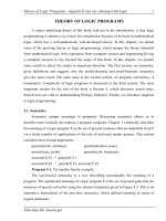
A major underlying theme of this book, laid out in the introduction, is that logic
programming is attractive as a basis for computation because of its basis in mathematical
logic, which has a well-understood, well-developed theory. In this chapter, we sketch
some of the growing theory of logic programming, which merges the theory inherited
from mathematical logic with experience from computer science and engineering.Giving
a complete account is way beyond the scope of this book. In this chapter, we present
some results to direct the reader in important direction. The first section, on semantics,
gives definitions and suggests why the model-theoretic and proof-theoretic semantics
give the same result. The main issue in the second section, on program correctness, is
termination. Complexity of logic programs is discussed in the third section. The most
important section for the rest of the book is Section 4, which discusses search trees.
Search trees are vital to understanding Prolog’s behavior. Finally, we introduce negation
in logic programming.
5.1. Semantics.
Semantics assigns meanings to programs. Discussing semantics allows us to
describe more formally the relation a program computes. Chapter 1 informally describes
the meaning of a logic program P as the set of ground instances that are deducible from P
via a finite number of applications of the rule of universal modus ponens. This section
considers more formal approaches.
parent(terach, abraham). parent(abraham, isaac).
parent(isaac, jacob). parent(jacob, benjamin).
ancestor(X,Y)
¬
parent(X,Y)
ancestor(X,Z)
¬
parent(X,Y), ancestor(Y,Z).
Program 5.1. Yet another family example.
The operational semantics is a way describing procedurally the meaning of a

program. The operational meaning of a logic program P is the set of ground goals that are
instances of queries solved by using the abstract interpreter given in Figure 4.2. This is an
alternative formulation of the previous semantics, which defined meaning in terms of
logical deduction.
Tiểu luận Hệ chuyên gia
Theory of Logic Programs - Nguyên lý của các chương trình logic 2
The declarative semantics of logic programs is based on the standard model-
theoretic semantics of first-order logic. In order to define it, some new terminology is
needed.
Definition
Let P be a logic program. The Herbrand universe of P, denoted U(P), is the set of
all ground terms that can be formed from the constants and function symbols appearing
in P.
In the section, we use two running examples-yet another family database example,
given as Program 5.1; and Program 3.1 defining the natural numbers, repeated here:
natural_number(0).
natural_number(s(X)) ← natural_number(X).
The Herbrand universe of Program 5.1 is the set of all constants appearing in the
program, namely, {terach, abraham, isaac, jacob, Benjamin}. If there are no function
symbols, the Herbrand universe is finite. In Program 3.1, there is one constant symbol, 0,
and one unary function symbol, s. The Herbrand universe of Program 3.1 is
{0,s(0),s(s(0)), . . .}. If no constants appear in a program, one is arbitrarily chosen.
Definition
The Herbrand base, denoted B(P), is the set of all ground goals that can be formed
from the predicates in P and the terms in the Herbrand universe.
There are two predicates, parent/2 and ancestor/2, in Program 5.1.
The Herbrand base of Program 5.1 consists of 25 goals for each predicate, where
each constant appears as each argument:
{parent(terach, terach), parent (terach, abraham),
parent(terach, isaac), parent (terach, jacob),

parent(terach, benjamin), parent (abraham, terach),
parent (abraham, abraham), parent (abraham, isaac ),
parent (abraham, jacob), parent (abraham, benjamin),
parent (isaac ,terach), parent (isaac, abraham),
parent (isaac, isaac), parent (isaac, jacob),
parent (isaac, benjamin), parent (jacob, terach),
parent (jacob, abraham), parent (jacob, isaac),
Tiểu luận Hệ chuyên gia
Theory of Logic Programs - Nguyên lý của các chương trình logic 3
parent (jacob, jacob), parent (jacob, benjamin),
parent (benjamin, terach), parent (benjamin, abraham),
parent (benjamin, isaac), parent (benjamin, jacob),
parent (benjamin, benjamin), ancestor (terach,terach),
ancestor(terach, abraham), ancestor(terach, isaac),
ancestor(terach, jacob), ancestor(terach, benjamin),
ancestor(abraham, terach), ancestor(abraham, abraham),
ancestor(abraham, isaac), ancestor(abraham, jacob),
ancestor(abraham, benjamin), ancestor(isaac, terach),
ancestor(isaac, abraham), ancestor(isaac, isaac),
ancestor(isaac, jacob), ancestor(isaac, benjamin),
ancestor(jacob, terach), ancestor(jacob, abraham),
ancestor(jacob, isaac), ancestor(jacob, jacob),
ancestor(jacob, benjamin), ancestor(benjamin, terach),
ancestor(benjamin, abraham), ancestor(benjamin, isaac),
ancestor(benjamin, jacob), ancestor(benjamin, benjamin)},
The Herbrand base is infinite if the Herbrand universe is. For Program 3.1, there is
one predicate, natural_number. The Herbrand base equals {natural_number(0),
natural_number(s(0)), }.
Definition
An interpretation for a logic program is a subset of the Herbrand base.

An interpretation assigns truth and falsity to the elements of the Herbrand base. A
goal in the Herbrand base is true with respect to an interpretation if it is a member of it,
false otherwise.
Definition
An interpretation I is a model for a logic program if for each ground instance of a
clause in the program
1
, ,
n
A B B¬
, A is in I if
1
, ,
n
B B
are in I.
Intuitively, models are interpretatinos that respect the declarative reading of the
clauses of a program.
For Program 3.1, natural_number(0) must be in every model, and natural_number(s(X))
is in the model if natural_number(X) is. Any model of program 3.1 thus includes the whole
Tiểu luận Hệ chuyên gia
Theory of Logic Programs - Nguyên lý của các chương trình logic 4
Herbrand base.
For Program 5.1, the facts parent(terach,abraham), parent(abraham,isaac),
parent(isaac,jacob) and parent(jacob,benjamin) must be in every model. A ground
instance of the goals ancestor(X,Y) is in the model if the corresponding instance of
parent(X,Y) is, by the first clause. So, for example, ancestor(terach, abraham) is in every
model. By the second clause, ancestor (X, Z) is in the model if parent (X, Y) and ancestor
(Y, Z) are.
It is easy to see that the intersection of two models for a logic program P is again a

model. This property allows the definition of the intersection of all models.
Definition
The model obtained as the intersection of all models is known as the minimal model
and denoted M(P). The minimal model is the declarative meaning of a logic program.
The declarative meaning of the program for natural_number, its minimal model, is the
complete Herbrand base {natural_number(0), natural_number(s(0)), natural_number(s(s(0))), }.
The declarative meaning of the program 5.1 is {parent(terach,abraham),
parent(abraham,isaac), parent(isaac,jacob) and parent(jacob,benjamin), ancestor(terach,
abraham), ancestor(abraham,isaac), ancestor(isaac,jacob), ancestor(jacob, benjamin),
ancestor(terach, isaac), ancestor(terach, jacob), ancestor(terach, benjamin),
ancestor(abraham, jacob), ancestor(abraham, benjamin) , ancestor(isaac, benjamin)}.
Let us consider the declarative meaning of append, defined as Program 3.15 and
repeated here:
append( [X/Xs], Ys, [X/Zs] ) - append(Xs, Ys, Zs).
append([ ], Ys, Ys).
The Herbrand universe is [ ], [[ ]], [[ ],[ ]], , namely, all lists that can be built
using the constant [ ]. The Herbrand base is all combinations of lists with the append
predicate. The declarative meaning is all ground instances of append ([ ], Xs,Xs), that is,
append ([ ], [ ], [ ]), append ([ ], [[ ]], [[ ]]), . . ., together with goals such as append ([[ ]],
[ ], [[ ]]), which are logically implied by application(s) of the rule. This is only a subset of
the Herbrand base. For example, append ([ ], [ ], [[ ]]) is not in the meaning of append but
is in the Herbrand base.
Denotational semantics assigns meaning to programs based on associating qith the
Tiểu luận Hệ chuyên gia
Theory of Logic Programs - Nguyên lý của các chương trình logic 5
program a function over the domain computed by the program. The meaning of the
program is defined as the least fixpoint of the function, if it exists. The domain of
compulations of logic programs is interpretations.
Definition
Given a logic program P, there is a natural mapping

p
T
from interpretations to
interpretations, defined as follows:
( ) { ( ) : 1, 2, , , 0,
p
T I AinB P A B B Bn n= ¬ ≥
is a ground instance of a clause in O, and
B1,…,Bn are in I}
The mapping is monotonic, since whenever an interpretation I is contained in an
interpretation J, then
( )
p
T I
is contained in
( )
p
T J
.
The mapping gives an alternative way of characterizing models. An interpretation I
is a model if and only if
( )
p
T I
is contained in I.
Besides being monotonic, the transformation is also continuous, a notion that will
not be defined here. These two properties ensure that for every logic program P, the
transformation
p
T

has a least fixpoint, which is the meaning assigned to P by its
denotational semantics.
Happily, all the different definitions of semantics are actually describing the same
object. The operational, denotational, and declarative semantics have been demonstrated
to be equivalent. This allows us to define the meaning of a logic program as its minimal
model.
5.2. Program Correctness.
Every logic program has a well-defined meaning, as discussed in Section 5.1. This
meaning is neither correct nor incorrect.
The meaning of the program, however, may or may not be what was intended by
the programer. Discussions of correctness must therefore take into consideration the
intended meaning of the program. Our previous discussion of proving correctness and
completeness similarly was with respect to an intended meaning of a program.
We recall the definitions from Chapter 1. An intended meaning of a program P is a
set of ground goals. We use intended meanings to denote the set of goals intended by the
Tiểu luận Hệ chuyên gia
Theory of Logic Programs - Nguyên lý của các chương trình logic 6
programer for the program to compute. A program P is complete with respect to an
intended meaning if M is contained in M(P). A program is thus correct and complete with
respect to an intended meaning if the two meanings coincide exactly.
Another important aspect of a logic program is whether it terminates.
Definition
A domain is a set of goals, not necessarily ground, closed under the instance
relation. That is, if A is in D and A’ is an instance of A, then A’ is in D as well.
Definition
A termination domain of a program P is a domain D such that every computation of
P on every goal in D terminates.
Usually, a useful program should have a termination domain that includes its
intended meaning. However, since the computation model of logic programs is liberal in
the order in which goals in the resolvent can be reduced. Most interesting logic programs

will not have interesting termination domains. This situation will improve when we
switch to Prolog. The restrictive model pf Prolog allows the programer to compose
nontrivial programs that terminate over useful domains.
Consider Program 3.1 defining the natural numbers. This program is terminating
over its Herbrand base. However, the program is nonterminating over the domain
{natural_number(X)}. This is caused by the possibility of the nonterminating
compulation depicted in the trace in Figure 5.1.
For any logic program, it is useful to find domains over which it is terminating. This
is usually difficult for recursive logic programs. We
natural_number (X) X=s(X1)
natural_number (X1) X1=s(X2)
natural_number (X2) X2=s(X3)
M
Figure 5.1 A nonterminating computation
need to describe recursive data types in a way that allows us to discuss termination.
Recall that a type, introduced in Chapter 3, is a set of terms.
Definition
A type is complete if the set is closed under the instance relation. With every
Tiểu luận Hệ chuyên gia
Theory of Logic Programs - Nguyên lý của các chương trình logic 7
complete type T we can associate an incomplete type IT, which is the set of terms that
have instances in T and instances not in T.
We illustrate the use of these definitions to find termination domains for the
recursive programs using recursive data types in Chapter 3. Specific instances of the
definitions of complete and incomplete types are given for natural numbers and lists. A
(complete) natural number is either the constant 0, or a term of the form
( )
n
s X
. An

incomplete natural number is either a variable, X, or term of the form
(0)
n
s
, where X is a
variable. Program 3.2 for
≤
is terminating for the domain consisting of goals where the
first and/or second argument is a complete natural number.
Definition
A list is complete if every instance satisfies the definition given in program 3.11. A
list is incompete if there are instances that satisfy this definition and instances that do not.
For example, the list [a,b,c] is complete (proved in Figure 3.3), while the variable X
is incomplete. Two more interesting examples: [a,X,c] is a complete list, although not
ground, whereas [a,b|Xs] is incomplete.
A termination domain for append is the set of goals where the first and/or the third
argument is a complete list. We discuss domains for other list-processing programs in
Section 7.2 on termination of Prolog programs.
5.2.1. Exercises for Section 5.2.
(i) Give a domain over which Program 3.3 for plus is terminating.
(ii) Define comlete and incomplete binary trees by anslogy with the definitions for
complete and incomplete lists.
5.3. Complexity.
We have analyzed informally the complexity of serveral logic programs, for
example,
≤
and plus (program 3.2 and 3.3) in the section on arithmetic, and append and
the two versions of reverse in the section on lists (Program 3.15 and 3.16). In the section,
we briefly describe more formal complexity measures.
The multiple uses of logic programs slightly change the nature of complexity

measures. Instead of looking at a particular use and specifying complexity in terms of the
Tiểu luận Hệ chuyên gia
Theory of Logic Programs - Nguyên lý của các chương trình logic 8
sizes of the inputs, we look at goals in the meaning and see how they were derived. A
natural measure of the complexity of a logic program is the length of the proofs it
generates for goals in its meaning.
Definition
The size of a term is the number of symbols in its textual representation.
Constants and variables, consisting of a single symbol, have size 1. The size of a
compound term is 1 more than the sum of the sizes of its arguments. For example, the list
[b] has size 3, [a,b] has size 5, and the goal append([a,b], [c,d], Xs) has size 12. In
general, a list of n elements has size 2 - n + 1.
Definition
A program P is of length complexity L(n) if for any goal G in the meaning of P of
size n there is a proof of G with respect to P of length less than equal to L(n).
Length complexity is related to the usual complexity measures in computer science.
For sequential realizations of the computation model, it corresponds to time complexity.
Program 3.15 for append has linear length complexity. This is demonstrated in Exercise
(i) at the end of this section.
The application of this measure to Prolog programs, as opposed to logic programs,
depends on using a unification algorithm without an occurs check. Consider the runtime
of the straightforward program for appending two lists. Appending two lists, as shown in
Figure 4.3, involves several unifications of append goals with the head of the append rule
append( [X/Xs], Ys, [X/Zs] ). At least three unifications, matching variables against
(possibly incomplete) lists, will be necessary. If the occurs check must be performed for
each, the argument lists must be searched. This is directly proportional to the size of the
input goal. However, if the occurs check is omitted, the unification time will be bounded
by a constant. The overall complexity of append becomes quadratic in the size of the
input lists with the occurs check, but only linear without it.
We introduce other useful measures related to proofs. Let R be a proof.

We define the depth of R to be the deepest invocation of a goal in the associated
reduction. The goal-size of R is the maximum size of any goal reduced.
Definition
A logic program P is of goal-size complexity G(n) if for any goal A in the meaning
Tiểu luận Hệ chuyên gia
Theory of Logic Programs - Nguyên lý của các chương trình logic 9
of P of size n, there is a proof of A with respect to P of goal-size less than or equal to
G(n).
Definition
A logic program P is of depth-complexity D(n) if for any goal A in the meaning of P
of size n, there is a proof of G with respect to P of depth
≤
D(n).
Goal-size complexity relates to space. Depth-complexity relates to space of what
needs to be remembered for sequential realizations, and to space and time complexity for
parallel realizations.
5.3.1 Exercises for Section 5.3.
(i) Show that the size of a goal in the meaning of append joining a list of length n to
one of length m to give list of length n + m is 4 – n + 4 – m + 4. Show that a proof tree
has m + 1 nodes. Hence show that append has linear complexity. Would the complexity
be altered if the type condition were added?
(ii) Show that Program 3.3 for plus has linear complexity.
(iii) Discuss the complexity of other logic programs.
5.4. Search Trees.
Computations of logic programs given so far resolve the issue of nonde- terminism
by always making the correct choice. For example, the com-plexity measures, based on
proof trees, assume that the correct clause can be chosen from the program o effect the
reduction. Another way of computationally modeling nondeterminism is by developing
all possible reductions in parallel. In this section, we discuss search trees, a formal-ism
for considering all possible computation paths.

Definition
A search tree of a goal G with respect to a program P is defined as follows. The root
of the tree is G. Nodes of the tree are (possibly con-functive) goals with one goal
selected. There is an edge leading from a node N for each clause in the program whose
head unifies with the selected goal. Each branch in the tree from the root is a computation
of G by P. leaves of the tree are success nodes, where the empty goal has been reached,
or failure nodes, where the selected goal at the node cannot be further reduced. Success
nodes correspond to solutions of the root of the tree.
Tiểu luận Hệ chuyên gia
Theory of Logic Programs - Nguyên lý của các chương trình logic 10
There are in general many search trees for a given goal with respect to a program.
Figure 5.2 shows two search trees for the query son(S,haran)? with respect to program
1.2. the two possibilities cor-respond tho the two choices of goal to reduce from the
resolvent father(haran,S), male(S). The trees are quite distinct, but both have a single
success branch corresponding tho the solution of the query S=lot. The respective success
branches are given as traces in figure 4.4.
We adopt some conventions when drawing search trees. The leftmost goal of a node
is always the selected one. This implies that the goals in derived goals may be permuted
so that the new goal to be selected for reduction is the first goal. The edges are labeled
with substitutions that are applied to the variables in the leftmost goal. These
substitutions are computed as part of the unication algorithm.
Search trees correspond closely to traces for deterministic computations. The traces
for the append query and Hanoi query given, respectively, in Figures 4.3 and 4.5 can be
easily made into search trees. This is Exercise(i) at the end of this section.
Search trees contain multiple success nodes if the query has multiple solutions.
Figure 5.3 contains the search tree for the query append(As,Bs,[a,b,c])? With respect to
program 3.15 for append, asking to split the list [a,b,c] into two. The solutions for As and
Bs are found by collecting the labels of the edges in the branch leading to the success
node. For example, in the figure, following the leftmost branch gives the solution{As =
[a,b,c], Bs = []}.

The number of success nodes in the same for any search tree of the given goal with
Tiểu luận Hệ chuyên gia
Theory of Logic Programs - Nguyên lý của các chương trình logic 11
respect to a program.
Search trees can have infinite branches, which correspond to nonterminating
computations. Consider the goal append(Xs,[c,d].Ys) with respect to the standard
program for append. The search tree is given in Figure 5.4. The infinite branch is the
nonterminating computation given in Figure 4.6.
Complexity measures can also be defined in terms of search trees. Prolog programs
perform a depth-first traversal of the search tree. Therefore, measures based on the size of
the search tree will bea more realistic measure of the complexity of prolog programs than
those based on the complexity of the proof tree. However, the complexity of the search
tree is much harder to analyze.
There is a deeper point lurking. The relation between proof trees and search trees is
the relation between nondeterministic computations and deterministic computations.
Whether the complexity classes difined via proof trees are equivalent to complexity
classes defined via search trees is a reformulation of the classic P=NP question in term of
logic programming.
5.4.1. Exercises for Section 5.4.
(i) Transform the traces of Figure 4.3 and 4.5 into search trees.
Tiểu luận Hệ chuyên gia
Theory of Logic Programs - Nguyên lý của các chương trình logic 12
(ii) Draw a search tree for the query sort([2,4,1],Xs)? Using permutation sort.
5.5. Negation in Logic Programming.
Logic programs are collections of rules and facts describing what is true. Untrue
facts are not expressed explicitly; they are omitted. When writing rules, it is often natural
to include negative conditions. For example, defining a bachelor as an unmarried male
could be written as
bachelor(X) ← male(X), not married(X).
if negation were allowed. In this section, we describe an extension to the logic

programming computation model that allows a limited form of negation.
Researchers have investigrated other extensions to logic programming to allow
disjunction, and indeed, arbitrary first-order formulae. Discussing them is beyond the
scope of this book. The most useful of the extensions is definitery negation.
We define a relation not G and give a semantics. The essence of logic programming
is that there is an efficient procedural semantics. There is a natural way to adapt the
procedural semantics to negation, namely by negation as failure. A goal G fails, (not G
succeeds), if G cannot be derived by the procedural semantics.
The relation not G is only a partial form of negation from first-order logic. The
Tiểu luận Hệ chuyên gia
Theory of Logic Programs - Nguyên lý của các chương trình logic 13
relation not uses the negation as failure rule. A goal not G will be assumed to be a
consequence of a program P if G is not a consequence of P.
Negation as failure can be characterized in term of search trees.
Definition
A search tree of a goal G with respect to a program P is finitely failed if it has no
success nodes or infinite branches. The finite failure set of a logic program P is the set of
goals G such that G has a finitely failed search tree with respect to P.
A goal not G is implied by a program P by the “nagation as failure” rule if G is in
the finite failure set of P.
Let us see a simple example. Consider the program consisting of two facts:
likes(abraham, pomegranates).
likes(isaac, pomegranates).
The goal not likes(sarah,pomegranates) follows from the program by negation as
failure. The search tree for the goal likes(sarah,pomegranates) has a single failure node.
Using negation as failure allows easy definition of many relations. For example, a
declarative definition of the relation disjoint(Xs,Ys) that two lists, Xs and Ys, have no
elements in common is possible as follows.
disjoint(Xs,Ys) ← not (member(X,Xs) , member(X,Ys)).
This reals: “Xs is disjoint from Ys if there is no element X that is a member of bith

Xs and Ys.
An intuitive understanding of negation as failure is fine for the programs in this
book using negation. There are semantic problems, however, especially when integrated
with other issues such as completeness and terminatio. Pointers to the literature are given
in Section 5.6, and Prolos’s implementation of negation as failure is discussed in Chapter
11.
5.6. Background.
The classic paper on the semantics of logic programs is of van Emden and
Kowalski(1976). Important extensions were given by Apt and van Emden(1982). In
particular, they showed that the choice of goal to reduce from the resolvent is arbitrary by
showing that the number of success nodes is an invariant for the search trees. Textbook
Tiểu luận Hệ chuyên gia
Theory of Logic Programs - Nguyên lý của các chương trình logic 14
accounts of the theory of logic programming discussing the equivalence between the
declarative and procedural semantics can be found in Apt(1990), Deville(1990), and
Lioyd(1987).
In Shapiro (1984), complexity measures for logic programs are compared with the
complexity of computations of alternating Turing machines. It is shown that goal-size is
linearly related to alternating space, the product of length and goal-size linearly related to
alternating tree-size, and the product of depth and goal-size is linearly related to
alternating time.
The classic name for search trees in the linearly is SLD trees. The name SLD was
coined by research in automatic theorem proving, whih preceded the birth of logic
programming. SLD resolution is a particular refinement of the resolution principle
introduced in Robinson(1965). Computations of logic programs can be interpreted as a
series of resolution steps, and in fact, SLD resolution steps, and are still
commonlydescribed thus in the literature. The acronym SLD stands for Selecting a
literal, using a Linear strategy, restricted to Definite clauses.
The first proof of the correctness and completenness of SLD resolution, albeit under
the name LUSH-resolution, was given by Hill (1974).

The subject of negation has received a large amount of attention and interest since
the inception of logic programming. The fundamental work on the semantics of negation
as failure is by Clark (1978). Clark’s results, establishing soundness, were extended by
jaffar et al. (1983), who proved the completeness of the rule.
The concept of negation as failure is a restricted version of the closed world
assumption as discussed in the database world. For more information see Reiter (1978).
There has been extensive research on characterizing negation in logic programming that
has not stabilized at this time. The reader should look up the latest logic programming
conference proceedings to find current thinking. A good place to start reading to
understand the issue is Kunen (1989).
Tiểu luận Hệ chuyên gia
Theory of Logic Programs - Nguyên lý của các chương trình logic 15
Leonardo Da Vinci. Portrait of the Florentine poet Bernardo Bellincioni, engated at
the Court of Ludovico Sforza. Woodcut, based on a drawing by Leonardo. From
Bellincioni’s Rime. Milan 1493.
Tiểu luận Hệ chuyên gia
Theory of Logic Programs - Nguyên lý của các chương trình logic 16
NGUYÊN LÝ CỦA CÁC CHƯƠNG TRÌNH LOGIC
Một chủ đề cơ bản chính của cuốn sách này, đã được nêu trong phần giới thiệu, đó
là lập trình logic, nó là một cơ sở tính toán hấp dẫn vì nó là cơ sở trong toán học logic,
với lý thuyết dễ hiểu, dễ phát triển. Trong chương này, chúng tôi phác họa một số phát
triển các lý thuyết lập trình logic, nó được hòa trộn giữa các lý thuyết được thừa kế từ
logic toán học với kinh nghiệm từ khoa học máy tính và kiến trúc máy tính. Để đưa ra
được một báo cáo hoàn chỉnh là việc vượt ra ngoài phạm vi của cuốn sách này. Trong
chương này, chúng tôi chỉ trình bày cho người đọc một số kết quả về các vấn đề quan
trọng. Phần đầu tiên, về mặt ngữ nghĩa, cho phép định nghĩa và gợi ý tại sao các mô hình-
lý thuyết và chứng minh-lý thuyết lại cho cùng một kết quả. Vấn đề chính trong phần thứ
hai, về tính đúng đắn của chương trình, là kết thúc (termination). Sự phức tạp của các
chương trình logic được thảo luận trong phần thứ ba. Phần quan trọng nhất trong các
phần còn lại của cuốn sách là phần 4, phần này nói về cây tìm kiếm (search trees). Cây

tìm kiếm là quan trọng để hiểu biết về hoạt động của Prolog. Cuối cùng, chúng tôi giới
thiệu về phủ định (negation) trong lập trình logic.
5.1. Ngữ nghĩa.
Ngữ nghĩa (semantic) gán ý nghĩa cho các chương trình. Thảo luận về ngữ nghĩa
cho phép chúng ta miêu tả mối quan hệ chính thức hơn một chương trình tính. Chương 1
mô tả ý nghĩa của một chương trình P logic như là tập hợp các thể nghiệm mặt (ground
instance) được suy dẫn từ P thông qua một số hữu hạn các ứng dụng của luật modus
ponens tổng quát. Phần này sẽ xem xét các cách tiếp cận nhiều hình thức.
parent(terach, abraham). parent(abraham, isaac).
parent(isaac, jacob). parent(jacob, benjamin).
ancestor(X,Y)
¬
parent(X,Y)
ancestor(X,Z)
¬
parent(X,Y), ancestor(Y,Z).
Chương trình 5.1. Ví dụ khác trong gia đình.
Các toán tử (operational) ngữ nghĩa là một cách để mô tả ý nghĩa của chương trình
theo thủ tục. Ý nghĩa của toán tử của một chương trình logic P là tập hợp các đích
ground đó là các thể nghiệm của các truy vấn được giải quyết bằng cách sử dụng trình
thông dịch trừu tượng nhất được cho trong hình 4.2. Đây là một công thức thay thế của
Tiểu luận Hệ chuyên gia
Theory of Logic Programs - Nguyên lý của các chương trình logic 17
ngữ nghĩa trước, trong đó đã được xác định ý nghĩa trong các hạng của luật suy dẫn logic.
Ngữ nghĩa tường thuật (declarative) của các chương trình logic là dựa trên mô hình
chuẩn lý thuyết ngữ nghĩa của logic mệnh lệnh đầu tiên (first-order logic). Để định nghĩa
chúng cần một số thuật ngữ mới.
Định nghĩa
Gải sử P là một chương trình logic. Không gian Herbrand (Herbrand universe) của
P, ký hiệu là U(P), là tập hợp của tất cả các hạng ground có thể được hình thành từ các

hằng số và các ký hiệu hàm (function symbol) xuất hiện trong P.
Trong phần này, chúng tôi sử dụng hai ví dụ chạy, cơ sở dữ liệu là một ví dụ khác
trong gia đình, được đưa ra như Chương trình 5.1 và chương trình 3.1 xác định số tự
nhiên, được lặp lại ở đây:
natural_number(0).
natural_number(s(X)) ← natural_number(X).
Không gian Herbrand của chương trình 5.1 là tập của tất cả các hằng số xuất hiện
trong chương trình, cụ thể là, {terach, abraham, isaac, jacob, benjamin). Nếu không có
các ký hiệu hàm, không gian Herbrand là hữu hạn. Trong chương trình 3.1, có một ký
hiệu hằng số, 0, và một ký hiệu hàm không xác định, s. Không gian Herbrand của chương
trình 3.1 là (0,s(0), s(s(0)), ). Nếu không có hằng số xuất hiện trong một chương trình,
thì lựa chọn tuỳ ý.
Định nghĩa
Cơ sở Herbrand (Herbrand base), ký hiệu là B(P), là tập hợp của tất cả các ground
goal có thể được hình thành từ các vị từ trong P và các hạng trong không gian Herbrand.
Có hai vị từ, parent/2 và ancestor/2, trong Chương trình 5.1. Cơ sở Herbrand của
chương trình 5.1 bao gồm 25 đích cho mỗi vị từ, trong đó mỗi hằng số xuất hiện như là
đối số:
{parent(terach, terach), parent (terach, abraham),
parent(terach, isaac), parent (terach, jacob),
parent(terach, benjamin), parent (abraham, terach),
parent (abraham, abraham), parent (abraham, isaac ),
parent (abraham, jacob), parent (abraham, benjamin),
parent (isaac ,terach), parent (isaac, abraham),
Tiểu luận Hệ chuyên gia
Theory of Logic Programs - Nguyên lý của các chương trình logic 18
parent (isaac, isaac), parent (isaac, jacob),
parent (isaac, benjamin), parent (jacob, terach),
parent (jacob, abraham), parent (jacob, isaac),
parent (jacob, jacob), parent (jacob, benjamin),

parent (benjamin, terach), parent (benjamin, abraham),
parent (benjamin, isaac), parent (benjamin, jacob),
parent (benjamin, benjamin), ancestor (terach,terach),
ancestor(terach, abraham), ancestor(terach, isaac),
ancestor(terach, jacob), ancestor(terach, benjamin),
ancestor(abraham, terach), ancestor(abraham, abraham),
ancestor(abraham, isaac), ancestor(abraham, jacob),
ancestor(abraham, benjamin), ancestor(isaac, terach),
ancestor(isaac, abraham), ancestor(isaac, isaac),
ancestor(isaac, jacob), ancestor(isaac, benjamin),
ancestor(jacob, terach), ancestor(jacob, abraham),
ancestor(jacob, isaac), ancestor(jacob, jacob),
ancestor(jacob, benjamin), ancestor(benjamin, terach),
ancestor(benjamin, abraham), ancestor(benjamin, isaac),
ancestor(benjamin, jacob), ancestor(benjamin, benjamin)},
Cơ sở Herbrand là vô hạn nếu là không gian Herbrand. Đối với chương trình 3.1, có
một vị từ natural_number. Cơ sở Herbrand bằng (natural_number (0), natural_number(s
(0)), }.
Định nghĩa
Một thông dịch (interpretation) cho một chương trình logic là một tập hợp con của
cơ sở Herbrand.
Một thông dịch gán đúng và sai cho các yếu tố của cơ sở Herbrand.
Một đích trong cơ sở Herbrand là đúng đối với một thông dịch nếu nó là một thành
viên của thông dịch, nếu không là sai.
Định nghĩa
Một thông dịch I là một mô hình (model) cho một chương trình logic nếu cho mỗi
thể nghiệm ground của một mệnh đề trong chương trình
1
, ,
n

A B B¬
, A là trong I, nếu
Tiểu luận Hệ chuyên gia
Theory of Logic Programs - Nguyên lý của các chương trình logic 19
1
, ,
n
B B
thuộc I.
Theo trực giác, các mô hình được thông dịch tôn trọng cách hiểu tường thuật của
các mệnh đề của một chương trình.
Đối với chương trình 3.1, natural_number(0) bắt buộc phải có trong mỗi mô hình, và
natural_number(s(X)) trong mô hình nếu natural_number (X) cũng trong mô hình. Bất kỳ mô
hình của chương trình 3.1 nào cũng bao gồm toàn bộ các cơ sở Herbrand.
Đối với chương trình 5.1, các sự kiện parent(terach,abraham), parent(abraham,isaac),
parent(isaac,jacob) và parent(jacob,benjamin) phải ở mỗi mô hình. Một thể nghiệm
ground của các đích ancestor(X,Y) là trong mô hình nếu thể nghiệm tương ứng của
parent(X,Y) cũng trong mô hình, bằng mệnh đề đầu tiên. Vì vậy, ancestor(terach, abraham)
là trong mỗi mô hình. Bằng mệnh đề thứ hai, ancestor(X, Z) là trong mô hình, nếu parent (X,
Y) và ancestor (Y, Z) cũng trong mô hình.
Dễ dàng để thấy rằng giao điểm của hai mô hình cho một chương trình logic P lại là một
mô hình. Điều này cho phép định nghĩa giao điểm của tất cả các mô hình.
Định nghĩa
Mô hình thu được là giao điểm của tất cả các mô hình được gọi là mô hình tối thiểu
(minimal model) ký hiệu là M(P). Các mô hình tối thiểu là ý nghĩa tường thuật (declarative
meaning) của một chương trình logic.
Ý nghĩa tường thuật của chương trình natural_number, mô hình tối thiểu của nó, là cơ sở
Herbrand hoàn thành {natural_number (0), natural_number (s (0)), natural_number (s (s
(0))), }.
Ý nghĩa tường thuật của chương trình 5.1 là {parent(terach,abraham),

parent(abraham,isaac), parent(isaac,jacob) and parent(jacob,benjamin), ancestor(terach,
abraham), ancestor(abraham,isaac), ancestor(isaac,jacob), ancestor(jacob, benjamin),
ancestor(terach, isaac), ancestor(terach, jacob), ancestor(terach, benjamin),
ancestor(abraham, jacob), ancestor(abraham, benjamin) , ancestor(isaac, benjamin)}.
Chúng ta hãy xem xét các ý nghĩa tường thuật của vị từ append (nối vào), định
nghĩa như chương trình 3.15 và được lặp lại ở đây:
append([X/Xs], Ys, [X/Zs]):- append(Xs, Ys, Zs).
append([ ], Ys, Ys).
Không gian Herbrand là [], [[]], [[], []], , cụ thể là, tất cả các danh sách mà có thể
Tiểu luận Hệ chuyên gia
Theory of Logic Programs - Nguyên lý của các chương trình logic 20
xây dựng bằng cách sử dụng hằng [ ]. Các cơ sở Herbrand là tất cả các kết hợp của các
danh sách với vị từ append. Ý nghĩa tường thuật là tất cả các thể nghiệm ground của
append([ ], Xs,Xs), có nghĩa là, append ([ ], [ ], [ ]), append ([ ], [[ ]], [[ ]]), , cùng với
các đích như append ([[ ]], [ ], [[ ]]), nó được ngụ ý logic bằng application(s) của luật.
Đây chỉ là một tập hợp của cơ sở Herbrand. Ví dụ, append([ ], [ ], [[ ]]) không thuộc ý
nghĩa của append nhưng lại thuộc cơ sở Herbrand.
Các ý nghĩa bao hàm (Denotational semantics) gán ý nghĩa cho các chương trình
dựa trên sự kết hợp với chương trình một hàm trên miền tính tới chương trình. Ý nghĩa
của chương trình được định nghĩa là số fixpoint ít nhất của hàm, nếu nó tồn tại. Các tên
miền của sự tính toán của các chương trình logic được thông dịch.
Định nghĩa
Cho một chương trình logic P, có một ánh xạ tự nhiên
p
T
từ thông dịch đến thông
dịch, được xác định như sau:
( ) { ( ) : 1, 2, , , 0,
p
T I AinB P A B B Bn n= ¬ ≥

là một thể nghiệm ground của một mệnh
đề trong O, và B
1
,…,B
n
thuộc I}
Ánh xạ là đơn điệu (monotonic), khi thông dịch I được bao hàm trong một thông
dịch J, sau đó
( )
p
T I
được bao hàm trong
( )
p
T J
.
Ánh xạ cho phép một cách khác để mô tả các mô hình. Một thông dịch I là một mô
hình nếu và chỉ nếu
( )
p
T I
được chứa trong I.
Không kể sự đơn điệu, sự biến đổi cũng là liên tục (continuous), một khái niệm mà
sẽ không được định nghĩa ở đây. Hai thuộc tính này đảm bảo cho mỗi chương trình logic
P. Biến đổi
p
T
là một fixpoint tối thiểu, nó là ý nghĩa được gán tới P bởi ngữ nghĩa bao
hàm của nó.
Thật là may mắn, tất cả các định nghĩa khác nhau về ngữ nghĩa mô tả cùng một đối

tượng. Ngữ nghĩa hoạt động, ý nghĩa, và tường thuật đã được chứng minh là tương
đương. Điều này cho phép chúng tôi xác định ý nghĩa của một chương trình logic như là
mô hình tối thiểu của nó.
5.2. Tính đúng đắn của chương trình.
Mỗi chương trình logic có một ý nghĩa xác định, như được thảo luận trong Phần
5.1. Điều này có nghĩa là chính xác hoặc không chính xác.
Tiểu luận Hệ chuyên gia
Theory of Logic Programs - Nguyên lý của các chương trình logic 21
Tuy nhiên, ý nghĩa của chương trình có thể hoặc không thể diễn đạt được những gì
đã được dự định bởi các lập trình viên. Thảo luận về sự đúng đắn đó thì phải đi vào xem
xét các ý nghĩa được dự định của chương trình. Thảo luận trước đây của chúng tôi về
việc chứng minh tính đúng đắn và đầy đủ là tương tự đối với một ý nghĩa dự định của
một chương trình.
Chúng ta nhắc lại các định nghĩa từ Chương 1. Một ý nghĩa được dự định (intended
meaning) của một chương trình P là một tập hợp các ground goal. Chúng tôi sử dụng ý
nghĩa được dự định để biểu thị tập hợp các đích dự định bởi lập trình viên cho chương
trình tính toán. Một chương trình P là hoàn thành đối với một ý nghĩa dự định nếu M
được chứa trong M(P). Một chương trình là như vậy, chính xác và đầy đủ đối với một ý
nghĩa dự định nếu hai ý nghĩa đó trùng nhau.
Một khía cạnh quan trọng khác của một chương trình logic là liệu nó chấm dứt
không.
Định nghĩa
Một miền (domain) là một tập hợp các đích, không nhất thiết phải ground, được
khép kín theo thể nghiệm quan hệ. Tức là, nếu A thuộc D và A' là một ví dụ của A, thì A'
thuộc D.
Định nghĩa
Một miền kết thúc (termination domain) của một chương trình P là một miền D sao
cho mọi tính toán của P trên mọi đích thuộc D kết thúc.
Thông thường, một chương trình hữu ích cần phải có một tên miền chấm dứt bao
gồm cả ý nghĩa được dự định của nó. Tuy nhiên, vì các mô hình tính toán của các chương

trình logic là tự do theo thứ tự nên các mục tiêu trong giải thức có thể được rút gọn. Chú
ý nhất là các chương trình logic sẽ không có miền chấm dứt. Tình trạng này sẽ cải thiện
khi chúng tôi chuyển sang Prolog. Các mô hình hạn chế của Prolog cho phép lập trình
viên soạn thảo các chương trình quan trọng chấm dứt với các tên miền hữu ích hơn.
Xem xét chương trình 3.1 xác định số tự nhiên. Chương trình này kết thúc trên cơ
sở Herbrand của nó. Tuy nhiên, chương trình không kết thúc trên miền
(natural_number(X)). Điều này là do khả năng của sự tính toán không kết thúc mô tả
trong các dấu vết trong hình 5.1.
Đối với bất kỳ chương trình logic, nó rất hữu ích để tìm các miền mà trên đó nó
Tiểu luận Hệ chuyên gia
Theory of Logic Programs - Nguyên lý của các chương trình logic 22
chấm dứt. Điều này thường khó khăn cho các chương trình đệ quy logic.
natural_number (X) X=s(X1)
natural_number (X1) X1=s(X2)
natural_number (X2) X2=s(X3)
M
Hình 5.1. Một tính toán không kết thúc
Chúng ta cần mô tả các kiểu dữ liệu đệ quy theo một cách mà cho phép chúng ta
thảo luận về việc chấm dứt.
Nhắc lại về kiểu, được giới thiệu trong Chương 3, là một tập các hạng.
Định nghĩa
Một kiểu (type) là hoàn thành (complete) nếu tập hợp được khép kín theo thể
nghiệm quan hệ. Với mỗi kiểu T hoàn thành, chúng ta có thể kết hợp một loại IT không
hoàn thành, đó là tập hợp các hạng có các thể nghiệm thuộc T và các thể nghiệm không
thuộc T.
Chúng tôi minh họa cho việc sử dụng của các định nghĩa này để tìm các miền cho
việc chấm dứt các chương trình đệ quy bằng cách sử dụng các loại dữ liệu đệ quy trong
Chương 3. Các thể nghiệm cụ thể của các định nghĩa về hoàn thành và không hoàn thành
được lấy cho các số tự nhiên và các danh sách. Một số tự nhiên (hoàn thành) hoặc là hằng
số 0, hoặc là một hạng có dạng

( )
n
s X
. Một số tự nhiên không hoàn thành hoặc là một
biến, X, hoặc là hạng có dạng
(0)
n
s
, trong đó X là một biến. Chương trình 3.2 cho
≤
là
kết thúc cho các miền bao gồm các đích, trong đó đầu tiên là and/or đối thứ hai là một số
tự nhiên hoàn thành.
Định nghĩa
Một danh sách là hoàn thành nếu mọi thể nghiệm đáp ứng được các định nghĩa
được đưa ra trong chương trình 3.11. Một danh sách là không hoàn thành nếu có bất kỳ
thể nghiệm nào không thoả mãn định nghĩa này.
Ví dụ, danh sách [a, b, c] là hoàn thành (đã chứng minh trong hình 3.3), trong khi
biến X là không hoàn thành. Hai ví dụ cần quan tâm khác: [a, X, c] là một danh sách
hoàn thành, mặc dù không phải ground, trong khi [a, b | Xs] là không hoàn thành.
Một miền chấm dứt cho vị từ append là tập hợp các đích, trong đó đầu tiên là and/or
đối số thứ ba là danh sách hoàn thành. Chúng ta thảo luận miền cho danh sách các
Tiểu luận Hệ chuyên gia
Theory of Logic Programs - Nguyên lý của các chương trình logic 23
chương trình khác tại Phần 7.2 về việc kết thúc của các chương trình Prolog.
5.2.1. Bài tập cho phần 5.2.
(i) Đưa ra một miền với chương trình 3.3 để vị từ plus (cộng) chấm dứt.
(ii) Định nghĩa cây nhị phân tìm kiếm hoàn thành và không hoàn thành bằng định
nghĩa danh sách hoàn thành và không hoàn thành.
5.3. Độ phức tạp.

Chúng tôi đã phân tích độ phức tạp của các chương trình logic, ví dụ,
≤
và plus
(chương trình 3.2 và 3.3) trong phần về số học ; append và hai phiên bản của reverse
(đảo ngược) trong phần danh sách (chương trình 3.15 và 3.16). Trong phần này, chúng
tôi mô tả ngắn gọn các biện pháp đo độ phức tạp chính thức.
Sử dụng nhiều chương trình logic một chút thay đổi bản chất của các biện pháp đo
độ phức tạp. Thay vì phải nhìn vào một số sử dụng chỉ định cụ thể và phức tạp trong các
hạng của các kích thước của các yếu tố đầu vào, chúng ta nhìn vào đích trong ý nghĩa và
xem sự xuất phát của chúng. Một biện pháp thường dùng để đo sự phức tạp của một
chương trình logic là chiều dài của các chứng minh mà nó tạo ra cho các đích trong ý
nghĩa của nó.
Định nghĩa
Kích thước (size) của một hạng là số ký hiệu trong văn bản đại diện của nó.
Hằng và biến, bao gồm một ký hiệu duy nhất, có kích thước 1. Kích thước của một
hạng phức hợp nhiều hơn tổng các kích thước của các đối số của nó. Ví dụ, danh sách [b]
có kích thước 3, [a,b] có kích thước 5, và đích append([a,b], [c,d], Xs) có kích thước 12.
Nói chung, một danh sách n phần tử có kích thước 2 - n + 1.
Định nghĩa
Một chương trình P có chiều dài phức tạp (length complexity) là L(n) nếu cho bất kỳ
đích G thuộc ý nghĩa của P của kích thước n có một chứng minh của G đối với P của
chiều dài ít hơn hoặc bằng L(n).
Chiều dài phức tạp liên quan đến các biện pháp phức tạp trong khoa học máy tính
thông thường. Đối với các thực hiện tuần tự của các mô hình tính toán, nó tương ứng với
thời gian phức tạp. Chương trình 3.15 cho vị từ append có chiều dài phức tạp tuyến tính.
Điều này được thể hiện ở bài tập (i) ở cuối phần này.
Tiểu luận Hệ chuyên gia
Theory of Logic Programs - Nguyên lý của các chương trình logic 24
Việc áp dụng các biện pháp này cho chương trình Prolog, trái với các chương trình
logic, phụ thuộc vào cách sử dụng một thuật toán thống nhất mà không xảy ra kiểm tra.

Xem xét thời gian chạy (runtime) của chương trình đơn giản cho việc nối thêm
(appending) hai danh sách. Nối thêm hai danh sách, như trong hình 4.3, bao gồm hợp
nhất việc nối thêm nhiều đích với phần đầu của luật append: append( [X/Xs], Ys,
[X/Zs]). Ít nhất có ba sự hợp nhất, kết hợp các biến (có thể không đầy đủ) bằng danh
sách, sẽ là cần thiết. Nếu xảy ra kiểm tra phải được thực hiện cho mỗi trường hợp, các
danh sách đối số phải được tìm kiếm. Chúng tỷ lệ thuận với kích thước của các đích đầu
vào. Tuy nhiên, nếu xảy ra trường hợp bỏ qua kiểm tra, thời gian hợp nhất sẽ được bao
quanh bởi một hằng số. Sự phức tạp tổng quan của append sẽ trở thành bậc hai trong các
kích thước của danh sách đầu vào với sự xuất hiện kiểm tra, nhưng chỉ có tuyến tính mà
không cần nó.
Chúng tôi giới thiệu các biện pháp hữu ích khác liên quan đến chứng minh. Để R là
một chứng minh.
Chúng tôi định nghĩa độ sâu của R là độ sâu nhất của một đích trong rút gọn liên
quan. Kích thước đích (goal-size) của R là kích thước tối đa của mọi đích đã được rút
gọn.
Định nghĩa
Một chương trình logic P là kích thước đích phức tạp (goal-size complexity) G(n)
nếu cho bất kỳ đích A nào thuộc ý nghĩa của P của kích thước n, có một chứng minh của
A với kích thước đích P nhỏ hơn hoặc bằng G(n).
Định nghĩa
Một chương trình logic P là độ sâu phức tạp D(n) nếu cho bất kỳ đích A nào thuộc ý
nghĩa của P của kích thước n, có một chứng minh của G đối với P của độ sâu
≤
D(n).
Kích thước đích phức tạp liên quan đến không gian. Độ sâu-phức tạp liên quan đến
không gian của những gì cần phải nhớ cho thực hiện tuần tự, và để không gian và thời
gian phức tạp cho thực hiện song song.
5.3.1. Bài tập cho phần 5.3.
(i) Cho biết kích thước của một đích thuộc ý nghĩa của append để hợp nhất một
danh sách có độ dài n với một trong các độ dài m để có danh sách có độ dài n + m là 4 - n

+ 4 - m + 4. Tìn một cây chứng minh có m + 1 nút. Từ đó cho biết độ phức tạp của
Tiểu luận Hệ chuyên gia
Theory of Logic Programs - Nguyên lý của các chương trình logic 25
append tuyến tính. Độ phức tạp có thể thay đổi nếu có các điều kiện được thêm vào
không?
(ii) Cho biết độ phức tạp của vị từ plus trong chương trình 3.3.
(iii) Thảo luận về sự phức tạp của các chương trình logic khác.
5.4. Cây tìm kiếm.
Tính toán của các chương trình logic cho đến nay chưa giải quyết được vấn đề đến
điểm cuối cùng bởi luôn có sự lựa chọn làm cho kết quả đúng. Ví dụ, các biện pháp phức
tạp, dựa trên cây chứng minh, giả định rằng các mệnh đề đúng có thể được chọn từ
chương trình để rút gọn. Một cách tính toán khác phát triển tất cả các khả năng có thể
được rút gọn song song. Trong phần này, chúng tôi thảo luận về cây tìm kiếm, một hình
thức chính thức, để xem xét tính toán tất cả các khả năng có thể xảy ra.
Định nghĩa
Một cây tìm kiếm một đích G đối với một chương trình P được định nghĩa như sau.
Gốc cây là G. Các nút của cây là các đích với một trong những đích đã chọn. Có một
cạnh từ một nút N cho mỗi mệnh đề trong chương trình có phần đầu thống nhất với đích
đã chọn. Mỗi nhánh trong cây từ gốc là một tính toán của G bởi P. Lá của cây là các nút
thành công, nơi mà đích đã được tìm thấy, hoặc các nút thất bại, nơi mà các đích được
chọn tại nút không thể tiếp tục rút gọn được. Các nút thành công tương ứng với các giải
thức của gốc cây.
Nói chung có nhiều cây tìm kiếm cho một đích đã cho đối với một chương trình.
Hình 5.2 cho thấy hai cây tìm kiếm cho truy vấn son(S, Haran)? đối với chương trình 1.2.
Có hai khả năng tương ứng với hai sự lựa chọn của mục tiêu rút gọn từ giải thức
father(haran,S), male(S). Các cây này là hơi khác biệt, nhưng cả hai có một nhánh thành
công duy nhất tương ứng với các giải pháp của truy vấn S=lot. Các nhánh thành công
tương ứng được cho như dấu vết trong hình 4.4.
Chúng ta áp dụng một số quy ước khi vẽ cây tìm kiếm. Đích tận cùng bên trái của
một nút luôn luôn là một trong những lựa chọn. Điều này ngụ ý rằng các đích trong các

đích xuất phát có thể được hoán vị để đích mới sẽ được chọn để rút gọn là đích đầu tiên.
Các cạnh được gắn nhãn với phép thế được áp dụng cho các biến trong các mục tiêu tận
cùng bên trái. Những phép thế được tính như một phần của thuật toán.
Cây tìm kiếm quan hệ chặt chẽ với các dấu vết để tính toán xác định. Các dấu vết
Tiểu luận Hệ chuyên gia