Econometrics
Bạn đang xem bản rút gọn của tài liệu. Xem và tải ngay bản đầy đủ của tài liệu tại đây (3.92 MB, 692 trang )
Econometrics
Michael Creel
Department of Economics and Economic History
Universitat Autònoma de Barcelona
February 2014
Contents
1 About this document 16
1.1 Prerequisites . . . . . . . . . . . . . . . . . . . . . . . . . . . . . . . . . . . . . . . . . . 16
1.2 Contents . . . . . . . . . . . . . . . . . . . . . . . . . . . . . . . . . . . . . . . . . . . . 17
1.3 Licenses . . . . . . . . . . . . . . . . . . . . . . . . . . . . . . . . . . . . . . . . . . . . 21
1.4 Obtaining the materials . . . . . . . . . . . . . . . . . . . . . . . . . . . . . . . . . . . 21
1.5 An easy way run the examples . . . . . . . . . . . . . . . . . . . . . . . . . . . . . . . . 21
2 Introduction: Economic and econometric models 23
3 Ordinary Least Squares 28
3.1 The Linear Model . . . . . . . . . . . . . . . . . . . . . . . . . . . . . . . . . . . . . . . 28
3.2 Estimation by least squares . . . . . . . . . . . . . . . . . . . . . . . . . . . . . . . . . 30
3.3 Geometric interpretation of least squares estimation . . . . . . . . . . . . . . . . . . . . 33
3.4 Influential observations and outliers . . . . . . . . . . . . . . . . . . . . . . . . . . . . . 38
3.5 Goodness of fit . . . . . . . . . . . . . . . . . . . . . . . . . . . . . . . . . . . . . . . . 41
3.6 The classical linear regression model . . . . . . . . . . . . . . . . . . . . . . . . . . . . 44
1
3.7 Small sample statistical properties of the least squares estimator . . . . . . . . . . . . . 46
3.8 Example: The Nerlove model . . . . . . . . . . . . . . . . . . . . . . . . . . . . . . . . 55
3.9 Exercises . . . . . . . . . . . . . . . . . . . . . . . . . . . . . . . . . . . . . . . . . . . . 61
4 Asymptotic properties of the least squares estimator 63
4.1 Consistency . . . . . . . . . . . . . . . . . . . . . . . . . . . . . . . . . . . . . . . . . . 64
4.2 Asymptotic normality . . . . . . . . . . . . . . . . . . . . . . . . . . . . . . . . . . . . 65
4.3 Asymptotic efficiency . . . . . . . . . . . . . . . . . . . . . . . . . . . . . . . . . . . . . 67
4.4 Exercises . . . . . . . . . . . . . . . . . . . . . . . . . . . . . . . . . . . . . . . . . . . . 68
5 Restrictions and hypothesis tests 69
5.1 Exact linear restrictions . . . . . . . . . . . . . . . . . . . . . . . . . . . . . . . . . . . 69
5.2 Testing . . . . . . . . . . . . . . . . . . . . . . . . . . . . . . . . . . . . . . . . . . . . . 76
5.3 The asymptotic equivalence of the LR, Wald and score tests . . . . . . . . . . . . . . . 85
5.4 Interpretation of test statistics . . . . . . . . . . . . . . . . . . . . . . . . . . . . . . . . 90
5.5 Confidence intervals . . . . . . . . . . . . . . . . . . . . . . . . . . . . . . . . . . . . . . 90
5.6 Bootstrapping . . . . . . . . . . . . . . . . . . . . . . . . . . . . . . . . . . . . . . . . . 92
5.7 Wald test for nonlinear restrictions: the delta method . . . . . . . . . . . . . . . . . . . 94
5.8 Example: the Nerlove data . . . . . . . . . . . . . . . . . . . . . . . . . . . . . . . . . . 99
5.9 Exercises . . . . . . . . . . . . . . . . . . . . . . . . . . . . . . . . . . . . . . . . . . . . 104
6 Stochastic regressors 108
6.1 Case 1 . . . . . . . . . . . . . . . . . . . . . . . . . . . . . . . . . . . . . . . . . . . . . 110
6.2 Case 2 . . . . . . . . . . . . . . . . . . . . . . . . . . . . . . . . . . . . . . . . . . . . . 111
6.3 Case 3 . . . . . . . . . . . . . . . . . . . . . . . . . . . . . . . . . . . . . . . . . . . . . 113
6.4 When are the assumptions reasonable? . . . . . . . . . . . . . . . . . . . . . . . . . . . 114
6.5 Exercises . . . . . . . . . . . . . . . . . . . . . . . . . . . . . . . . . . . . . . . . . . . . 116
7 Data problems 117
7.1 Collinearity . . . . . . . . . . . . . . . . . . . . . . . . . . . . . . . . . . . . . . . . . . 117
7.2 Measurement error . . . . . . . . . . . . . . . . . . . . . . . . . . . . . . . . . . . . . . 136
7.3 Missing observations . . . . . . . . . . . . . . . . . . . . . . . . . . . . . . . . . . . . . 142
7.4 Missing regressors . . . . . . . . . . . . . . . . . . . . . . . . . . . . . . . . . . . . . . . 148
7.5 Exercises . . . . . . . . . . . . . . . . . . . . . . . . . . . . . . . . . . . . . . . . . . . . 149
8 Functional form and nonnested tests 150
8.1 Flexible functional forms . . . . . . . . . . . . . . . . . . . . . . . . . . . . . . . . . . . 152
8.2 Testing nonnested hypotheses . . . . . . . . . . . . . . . . . . . . . . . . . . . . . . . . 164
9 Generalized least squares 168
9.1 Effects of nonspherical disturbances on the OLS estimator . . . . . . . . . . . . . . . . 169
9.2 The GLS estimator . . . . . . . . . . . . . . . . . . . . . . . . . . . . . . . . . . . . . . 173
9.3 Feasible GLS . . . . . . . . . . . . . . . . . . . . . . . . . . . . . . . . . . . . . . . . . 177
9.4 Heteroscedasticity . . . . . . . . . . . . . . . . . . . . . . . . . . . . . . . . . . . . . . . 179
9.5 Autocorrelation . . . . . . . . . . . . . . . . . . . . . . . . . . . . . . . . . . . . . . . . 198
9.6 Exercises . . . . . . . . . . . . . . . . . . . . . . . . . . . . . . . . . . . . . . . . . . . . 229
10 Endogeneity and simultaneity 235
10.1 Simultaneous equations . . . . . . . . . . . . . . . . . . . . . . . . . . . . . . . . . . . . 235
10.2 Reduced form . . . . . . . . . . . . . . . . . . . . . . . . . . . . . . . . . . . . . . . . . 240
10.3 Estimation of the reduced form equations . . . . . . . . . . . . . . . . . . . . . . . . . . 243
10.4 Bias and inconsistency of OLS estimation of a structural equation . . . . . . . . . . . . 247
10.5 Note about the rest of this chaper . . . . . . . . . . . . . . . . . . . . . . . . . . . . . . 249
10.6 Identification by exclusion restrictions . . . . . . . . . . . . . . . . . . . . . . . . . . . . 249
10.7 2SLS . . . . . . . . . . . . . . . . . . . . . . . . . . . . . . . . . . . . . . . . . . . . . . 260
10.8 Testing the overidentifying restrictions . . . . . . . . . . . . . . . . . . . . . . . . . . . 264
10.9 System methods of estimation . . . . . . . . . . . . . . . . . . . . . . . . . . . . . . . . 270
10.10Example: Klein’s Model 1 . . . . . . . . . . . . . . . . . . . . . . . . . . . . . . . . . . 278
11 Numeric optimization methods 284
11.1 Search . . . . . . . . . . . . . . . . . . . . . . . . . . . . . . . . . . . . . . . . . . . . . 285
11.2 Derivative-based methods . . . . . . . . . . . . . . . . . . . . . . . . . . . . . . . . . . 287
11.3 Simulated Annealing . . . . . . . . . . . . . . . . . . . . . . . . . . . . . . . . . . . . . 297
11.4 A practical example: Maximum likelihood estimation using count data: The MEPS
data and the Poisson model . . . . . . . . . . . . . . . . . . . . . . . . . . . . . . . . . 297
11.5 Numeric optimization: pitfalls . . . . . . . . . . . . . . . . . . . . . . . . . . . . . . . . 301
11.6 Exercises . . . . . . . . . . . . . . . . . . . . . . . . . . . . . . . . . . . . . . . . . . . . 307
12 Asymptotic properties of extremum estimators 308
12.1 Extremum estimators . . . . . . . . . . . . . . . . . . . . . . . . . . . . . . . . . . . . . 308
12.2 Existence . . . . . . . . . . . . . . . . . . . . . . . . . . . . . . . . . . . . . . . . . . . 312
12.3 Consistency . . . . . . . . . . . . . . . . . . . . . . . . . . . . . . . . . . . . . . . . . . 312
12.4 Example: Consistency of Least Squares . . . . . . . . . . . . . . . . . . . . . . . . . . . 320
12.5 Example: Inconsistency of Misspecified Least Squares . . . . . . . . . . . . . . . . . . . 322
12.6 Example: Linearization of a nonlinear model . . . . . . . . . . . . . . . . . . . . . . . . 322
12.7 Asymptotic Normality . . . . . . . . . . . . . . . . . . . . . . . . . . . . . . . . . . . . 326
12.8 Example: Classical linear model . . . . . . . . . . . . . . . . . . . . . . . . . . . . . . . 329
12.9 Exercises . . . . . . . . . . . . . . . . . . . . . . . . . . . . . . . . . . . . . . . . . . . . 331
13 Maximum likelihood estimation 332
13.1 The likelihood function . . . . . . . . . . . . . . . . . . . . . . . . . . . . . . . . . . . . 333
13.2 Consistency of MLE . . . . . . . . . . . . . . . . . . . . . . . . . . . . . . . . . . . . . 338
13.3 The score function . . . . . . . . . . . . . . . . . . . . . . . . . . . . . . . . . . . . . . 339
13.4 Asymptotic normality of MLE . . . . . . . . . . . . . . . . . . . . . . . . . . . . . . . . 341
13.5 The information matrix equality . . . . . . . . . . . . . . . . . . . . . . . . . . . . . . . 345
13.6 The Cramér-Rao lower bound . . . . . . . . . . . . . . . . . . . . . . . . . . . . . . . . 350
13.7 Likelihood ratio-type tests . . . . . . . . . . . . . . . . . . . . . . . . . . . . . . . . . . 353
13.8 Examples . . . . . . . . . . . . . . . . . . . . . . . . . . . . . . . . . . . . . . . . . . . 355
13.9 Exercises . . . . . . . . . . . . . . . . . . . . . . . . . . . . . . . . . . . . . . . . . . . . 372
14 Generalized method of moments 375
14.1 Motivation . . . . . . . . . . . . . . . . . . . . . . . . . . . . . . . . . . . . . . . . . . . 375
14.2 Definition of GMM estimator . . . . . . . . . . . . . . . . . . . . . . . . . . . . . . . . 381
14.3 Consistency . . . . . . . . . . . . . . . . . . . . . . . . . . . . . . . . . . . . . . . . . . 382
14.4 Asymptotic normality . . . . . . . . . . . . . . . . . . . . . . . . . . . . . . . . . . . . 383
14.5 Choosing the weighting matrix . . . . . . . . . . . . . . . . . . . . . . . . . . . . . . . . 386
14.6 Estimation of the variance-covariance matrix . . . . . . . . . . . . . . . . . . . . . . . . 390
14.7 Estimation using conditional moments . . . . . . . . . . . . . . . . . . . . . . . . . . . 395
14.8 Estimation using dynamic moment conditions . . . . . . . . . . . . . . . . . . . . . . . 398
14.9 A specification test . . . . . . . . . . . . . . . . . . . . . . . . . . . . . . . . . . . . . . 399
14.10Example: Generalized instrumental variables estimator . . . . . . . . . . . . . . . . . . 402
14.11Nonlinear simultaneous equations . . . . . . . . . . . . . . . . . . . . . . . . . . . . . . 413
14.12Maximum likelihood . . . . . . . . . . . . . . . . . . . . . . . . . . . . . . . . . . . . . 414
14.13Example: OLS as a GMM estimator - the Nerlove model again . . . . . . . . . . . . . . 417
14.14Example: The MEPS data . . . . . . . . . . . . . . . . . . . . . . . . . . . . . . . . . . 417
14.15Example: The Hausman Test . . . . . . . . . . . . . . . . . . . . . . . . . . . . . . . . 420
14.16Application: Nonlinear rational expectations . . . . . . . . . . . . . . . . . . . . . . . . 429
14.17Empirical example: a portfolio model . . . . . . . . . . . . . . . . . . . . . . . . . . . . 434
14.18Exercises . . . . . . . . . . . . . . . . . . . . . . . . . . . . . . . . . . . . . . . . . . . . 438
15 Models for time series data 442
15.1 ARMA models . . . . . . . . . . . . . . . . . . . . . . . . . . . . . . . . . . . . . . . . 445
15.2 VAR models . . . . . . . . . . . . . . . . . . . . . . . . . . . . . . . . . . . . . . . . . . 453
15.3 ARCH, GARCH and Stochastic volatility . . . . . . . . . . . . . . . . . . . . . . . . . . 455
15.4 State space models . . . . . . . . . . . . . . . . . . . . . . . . . . . . . . . . . . . . . . 461
15.5 Nonstationarity and cointegration . . . . . . . . . . . . . . . . . . . . . . . . . . . . . . 462
15.6 Exercises . . . . . . . . . . . . . . . . . . . . . . . . . . . . . . . . . . . . . . . . . . . . 462
16 Bayesian methods 463
16.1 Definitions . . . . . . . . . . . . . . . . . . . . . . . . . . . . . . . . . . . . . . . . . . . 464
16.2 Philosophy, etc. . . . . . . . . . . . . . . . . . . . . . . . . . . . . . . . . . . . . . . . . 465
16.3 Example . . . . . . . . . . . . . . . . . . . . . . . . . . . . . . . . . . . . . . . . . . . . 467
16.4 Theory . . . . . . . . . . . . . . . . . . . . . . . . . . . . . . . . . . . . . . . . . . . . . 468
16.5 Computational methods . . . . . . . . . . . . . . . . . . . . . . . . . . . . . . . . . . . 470
16.6 Examples . . . . . . . . . . . . . . . . . . . . . . . . . . . . . . . . . . . . . . . . . . . 474
16.7 Exercises . . . . . . . . . . . . . . . . . . . . . . . . . . . . . . . . . . . . . . . . . . . . 482
17 Introduction to panel data 483
17.1 Generalities . . . . . . . . . . . . . . . . . . . . . . . . . . . . . . . . . . . . . . . . . . 483
17.2 Static models and correlations between variables . . . . . . . . . . . . . . . . . . . . . . 486
17.3 Estimation of the simple linear panel model . . . . . . . . . . . . . . . . . . . . . . . . 488
17.4 Dynamic panel data . . . . . . . . . . . . . . . . . . . . . . . . . . . . . . . . . . . . . 492
17.5 Exercises . . . . . . . . . . . . . . . . . . . . . . . . . . . . . . . . . . . . . . . . . . . . 497
18 Quasi-ML 499
18.1 Consistent Estimation of Variance Components . . . . . . . . . . . . . . . . . . . . . . 502
18.2 Example: the MEPS Data . . . . . . . . . . . . . . . . . . . . . . . . . . . . . . . . . . 504
18.3 Exercises . . . . . . . . . . . . . . . . . . . . . . . . . . . . . . . . . . . . . . . . . . . . 517
19 Nonlinear least squares (NLS) 519
19.1 Introduction and definition . . . . . . . . . . . . . . . . . . . . . . . . . . . . . . . . . . 519
19.2 Identification . . . . . . . . . . . . . . . . . . . . . . . . . . . . . . . . . . . . . . . . . 522
19.3 Consistency . . . . . . . . . . . . . . . . . . . . . . . . . . . . . . . . . . . . . . . . . . 524
19.4 Asymptotic normality . . . . . . . . . . . . . . . . . . . . . . . . . . . . . . . . . . . . 524
19.5 Example: The Poisson model for count data . . . . . . . . . . . . . . . . . . . . . . . . 526
19.6 The Gauss-Newton algorithm . . . . . . . . . . . . . . . . . . . . . . . . . . . . . . . . 528
19.7 Application: Limited dependent variables and sample selection . . . . . . . . . . . . . . 530
20 Nonparametric inference 535
20.1 Possible pitfalls of parametric inference: estimation . . . . . . . . . . . . . . . . . . . . 535
20.2 Possible pitfalls of parametric inference: hypothesis testing . . . . . . . . . . . . . . . . 541
20.3 Estimation of regression functions . . . . . . . . . . . . . . . . . . . . . . . . . . . . . . 543
20.4 Density function estimation . . . . . . . . . . . . . . . . . . . . . . . . . . . . . . . . . 561
20.5 Examples . . . . . . . . . . . . . . . . . . . . . . . . . . . . . . . . . . . . . . . . . . . 567
20.6 Exercises . . . . . . . . . . . . . . . . . . . . . . . . . . . . . . . . . . . . . . . . . . . . 574
21 Quantile regression 575
22 Simulation-based methods for estimation and inference 581
22.1 Motivation . . . . . . . . . . . . . . . . . . . . . . . . . . . . . . . . . . . . . . . . . . . 582
22.2 Simulated maximum likelihood (SML) . . . . . . . . . . . . . . . . . . . . . . . . . . . 589
22.3 Method of simulated moments (MSM) . . . . . . . . . . . . . . . . . . . . . . . . . . . 593
22.4 Efficient method of moments (EMM) . . . . . . . . . . . . . . . . . . . . . . . . . . . . 597
22.5 Indirect likelihood inference . . . . . . . . . . . . . . . . . . . . . . . . . . . . . . . . . 604
22.6 Examples . . . . . . . . . . . . . . . . . . . . . . . . . . . . . . . . . . . . . . . . . . . 611
22.7 Exercises . . . . . . . . . . . . . . . . . . . . . . . . . . . . . . . . . . . . . . . . . . . . 618
23 Parallel programming for econometrics 619
23.1 Example problems . . . . . . . . . . . . . . . . . . . . . . . . . . . . . . . . . . . . . . 621
24 Introduction to Octave 628
24.1 Getting started . . . . . . . . . . . . . . . . . . . . . . . . . . . . . . . . . . . . . . . . 628
24.2 A short introduction . . . . . . . . . . . . . . . . . . . . . . . . . . . . . . . . . . . . . 629
24.3 If you’re running a Linux installation . . . . . . . . . . . . . . . . . . . . . . . . . . . 631
25 Notation and Review 632
25.1 Notation for differentiation of vectors and matrices . . . . . . . . . . . . . . . . . . . . 632
25.2 Convergenge modes . . . . . . . . . . . . . . . . . . . . . . . . . . . . . . . . . . . . . 634
25.3 Rates of convergence and asymptotic equality . . . . . . . . . . . . . . . . . . . . . . . 638
26 Licenses 642
26.1 The GPL . . . . . . . . . . . . . . . . . . . . . . . . . . . . . . . . . . . . . . . . . . . 642
26.2 Creative Commons . . . . . . . . . . . . . . . . . . . . . . . . . . . . . . . . . . . . . . 658
27 The attic 666
27.1 Hurdle models . . . . . . . . . . . . . . . . . . . . . . . . . . . . . . . . . . . . . . . . . 677
List of Figures
1.1 Octave . . . . . . . . . . . . . . . . . . . . . . . . . . . . . . . . . . . . . . . . . . . . . 19
1.2 L
Y
X . . . . . . . . . . . . . . . . . . . . . . . . . . . . . . . . . . . . . . . . . . . . . . 20
3.1 Typical data, Classical Model . . . . . . . . . . . . . . . . . . . . . . . . . . . . . . . . 31
3.2 Example OLS Fit . . . . . . . . . . . . . . . . . . . . . . . . . . . . . . . . . . . . . . . 34
3.3 The fit in observation space . . . . . . . . . . . . . . . . . . . . . . . . . . . . . . . . . 35
3.4 Detection of influential observations . . . . . . . . . . . . . . . . . . . . . . . . . . . . . 40
3.5 Uncentered R
2
. . . . . . . . . . . . . . . . . . . . . . . . . . . . . . . . . . . . . . . . . 43
3.6 Unbiasedness of OLS under classical assumptions . . . . . . . . . . . . . . . . . . . . . 48
3.7 Biasedness of OLS when an assumption fails . . . . . . . . . . . . . . . . . . . . . . . . 49
3.8 Gauss-Markov Result: The OLS estimator . . . . . . . . . . . . . . . . . . . . . . . . . 53
3.9 Gauss-Markov Resul: The split sample estimator . . . . . . . . . . . . . . . . . . . . . 54
5.1 Joint and Individual Confidence Regions . . . . . . . . . . . . . . . . . . . . . . . . . . 91
5.2 RTS as a function of firm size . . . . . . . . . . . . . . . . . . . . . . . . . . . . . . . . 105
7.1 s(β) when there is no collinearity . . . . . . . . . . . . . . . . . . . . . . . . . . . . . . 125
10
7.2 s(β) when there is collinearity . . . . . . . . . . . . . . . . . . . . . . . . . . . . . . . . 126
7.3 Collinearity: Monte Carlo results . . . . . . . . . . . . . . . . . . . . . . . . . . . . . . 130
7.4 OLS and Ridge regression . . . . . . . . . . . . . . . . . . . . . . . . . . . . . . . . . . 136
7.5 ˆρ − ρ with and without measurement error . . . . . . . . . . . . . . . . . . . . . . . . . 142
7.6 Sample selection bias . . . . . . . . . . . . . . . . . . . . . . . . . . . . . . . . . . . . . 146
9.1 Rejection frequency of 10% t-test, H0 is true. . . . . . . . . . . . . . . . . . . . . . . . 172
9.2 Motivation for GLS correction when there is HET . . . . . . . . . . . . . . . . . . . . . 188
9.3 Residuals, Nerlove model, sorted by firm size . . . . . . . . . . . . . . . . . . . . . . . . 193
9.4 Residuals from time trend for CO2 data . . . . . . . . . . . . . . . . . . . . . . . . . . 201
9.5 Autocorrelation induced by misspecification . . . . . . . . . . . . . . . . . . . . . . . . 203
9.6 Efficiency of OLS and FGLS, AR1 errors . . . . . . . . . . . . . . . . . . . . . . . . . . 213
9.7 Durbin-Watson critical values . . . . . . . . . . . . . . . . . . . . . . . . . . . . . . . . 220
9.8 Dynamic model with MA(1) errors . . . . . . . . . . . . . . . . . . . . . . . . . . . . . 224
9.9 Residuals of simple Nerlove model . . . . . . . . . . . . . . . . . . . . . . . . . . . . . . 225
9.10 OLS residuals, Klein consumption equation . . . . . . . . . . . . . . . . . . . . . . . . . 228
10.1 Exogeneity and Endogeneity (adapted from Cameron and Trivedi) . . . . . . . . . . . . 236
11.1 Search method . . . . . . . . . . . . . . . . . . . . . . . . . . . . . . . . . . . . . . . . 286
11.2 Increasing directions of search . . . . . . . . . . . . . . . . . . . . . . . . . . . . . . . . 289
11.3 Newton iteration . . . . . . . . . . . . . . . . . . . . . . . . . . . . . . . . . . . . . . . 292
11.4 Using Sage to get analytic derivatives . . . . . . . . . . . . . . . . . . . . . . . . . . . . 296
11.5 Mountains with low fog . . . . . . . . . . . . . . . . . . . . . . . . . . . . . . . . . . . . 302
11.6 A foggy mountain . . . . . . . . . . . . . . . . . . . . . . . . . . . . . . . . . . . . . . . 303
13.1 Dwarf mongooses . . . . . . . . . . . . . . . . . . . . . . . . . . . . . . . . . . . . . . . 367
13.2 Life expectancy of mongooses, Weibull model . . . . . . . . . . . . . . . . . . . . . . . 368
13.3 Life expectancy of mongooses, mixed Weibull model . . . . . . . . . . . . . . . . . . . . 370
14.1 Method of Moments . . . . . . . . . . . . . . . . . . . . . . . . . . . . . . . . . . . . . 376
14.2 Asymptotic Normality of GMM estimator, χ
2
example . . . . . . . . . . . . . . . . . . 387
14.3 Inefficient and Efficient GMM estimators, χ
2
data . . . . . . . . . . . . . . . . . . . . . 391
14.4 GIV estimation results for ˆρ − ρ, dynamic model with measurement error . . . . . . . . 411
14.5 OLS . . . . . . . . . . . . . . . . . . . . . . . . . . . . . . . . . . . . . . . . . . . . . . 421
14.6 IV . . . . . . . . . . . . . . . . . . . . . . . . . . . . . . . . . . . . . . . . . . . . . . . 422
14.7 Incorrect rank and the Hausman test . . . . . . . . . . . . . . . . . . . . . . . . . . . . 427
15.1 NYSE weekly close price, 100 ×log differences . . . . . . . . . . . . . . . . . . . . . . . 457
16.1 Bayesian estimation, exponential likelihood, lognormal prior . . . . . . . . . . . . . . . 468
16.2 Chernozhukov and Hong, Theorem 2 . . . . . . . . . . . . . . . . . . . . . . . . . . . . 469
16.3 Metropolis-Hastings MCMC, exponential likelihood, lognormal prior . . . . . . . . . . . 475
16.4 Data from RBC model . . . . . . . . . . . . . . . . . . . . . . . . . . . . . . . . . . . . 480
16.5 BVAR residuals, with separation . . . . . . . . . . . . . . . . . . . . . . . . . . . . . . 481
20.1 True and simple approximating functions . . . . . . . . . . . . . . . . . . . . . . . . . . 537
20.2 True and approximating elasticities . . . . . . . . . . . . . . . . . . . . . . . . . . . . . 538
20.3 True function and more flexible approximation . . . . . . . . . . . . . . . . . . . . . . . 540
20.4 True elasticity and more flexible approximation . . . . . . . . . . . . . . . . . . . . . . 541
20.5 Negative binomial raw moments . . . . . . . . . . . . . . . . . . . . . . . . . . . . . . . 565
20.6 Kernel fitted OBDV usage versus AGE . . . . . . . . . . . . . . . . . . . . . . . . . . . 568
20.7 Dollar-Euro . . . . . . . . . . . . . . . . . . . . . . . . . . . . . . . . . . . . . . . . . . 571
20.8 Dollar-Yen . . . . . . . . . . . . . . . . . . . . . . . . . . . . . . . . . . . . . . . . . . . 572
20.9 Kernel regression fitted conditional second moments, Yen/Dollar and Euro/Dollar . . . 573
21.1 Inverse CDF for N(0,1) . . . . . . . . . . . . . . . . . . . . . . . . . . . . . . . . . . . . 577
21.2 Quantile regression results . . . . . . . . . . . . . . . . . . . . . . . . . . . . . . . . . . 580
23.1 Speedups from parallelization . . . . . . . . . . . . . . . . . . . . . . . . . . . . . . . . 626
24.1 Running an Octave program . . . . . . . . . . . . . . . . . . . . . . . . . . . . . . . . . 630
List of Tables
17.1 Dynamic panel data model. Bias. Source for ML and II is Gouriéroux, Phillips and
Yu, 2010, Table 2. SBIL, SMIL and II are exactly identified, using the ML auxiliary
statistic. SBIL(OI) and SMIL(OI) are overidentified, using both the naive and ML
auxiliary statistics. . . . . . . . . . . . . . . . . . . . . . . . . . . . . . . . . . . . . . . 494
17.2 Dynamic panel data model. RMSE. Source for ML and II is Gouriéroux, Phillips and
Yu, 2010, Table 2. SBIL, SMIL and II are exactly identified, using the ML auxiliary
statistic. SBIL(OI) and SMIL(OI) are overidentified, using both the naive and ML
auxiliary statistics. . . . . . . . . . . . . . . . . . . . . . . . . . . . . . . . . . . . . . . 495
18.1 Marginal Variances, Sample and Estimated (Poisson) . . . . . . . . . . . . . . . . . . . 505
18.2 Marginal Variances, Sample and Estimated (NB-II) . . . . . . . . . . . . . . . . . . . . 512
18.3 Information Criteria, OBDV . . . . . . . . . . . . . . . . . . . . . . . . . . . . . . . . . 516
22.1 True parameter values and bound of priors . . . . . . . . . . . . . . . . . . . . . . . . . 610
22.2 Monte Carlo results, bias corrected estimators . . . . . . . . . . . . . . . . . . . . . . . 610
27.1 Actual and Poisson fitted frequencies . . . . . . . . . . . . . . . . . . . . . . . . . . . . 677
14
27.2 Actual and Hurdle Poisson fitted frequencies . . . . . . . . . . . . . . . . . . . . . . . . 683
Chapter 1
About this document
1.1 Prerequisites
These notes have been prepared under the assumption that the reader understands basic statistics,
linear algebra, and mathematical optimization. There are many sources for this material, one are
the appendices to Introductory Econometrics: A Modern Approach by Jeffrey Wooldridge. It is the
student’s resposibility to get up to speed on this material, it will not be covered in class
This document integrates lecture notes for a one year graduate level course with computer programs
that illustrate and apply the methods that are studied. The immediate availability of executable (and
modifiable) example programs when using the PDF version of the document is a distinguishing feature
of these notes. If printed, the document is a somewhat terse approximation to a textbook. These notes
are not intended to be a perfect substitute for a printed textbook. If you are a student of mine, please
note that last sentence carefully. There are many good textbooks available. Students taking my courses
should read the appropriate sections from at least one of the following books (or other textbooks with
16
similar level and content)
• Cameron, A.C. and P.K. Trivedi, Microeconometrics - Methods and Applications
• Davidson, R. and J.G. MacKinnon, Econometric Theory and Methods
• Gallant, A.R., An Introduction to Econometric Theory
• Hamilton, J.D., Time Series Analysis
• Hayashi, F., Econometrics
A more introductory-level reference is Introductory Econometrics: A Modern Approach by Jeffrey
Wooldridge.
1.2 Contents
With respect to contents, the emphasis is on estimation and inference within the world of stationary
data. If you take a moment to read the licensing information in the next section, you’ll see that you
are free to copy and modify the document. If anyone would like to contribute material that expands
the contents, it would be very welcome. Error corrections and other additions are also welcome.
The integrated examples (they are on-line here and the support files are here) are an important
part of these notes. GNU Octave (www.octave.org) has been used for most of the example programs,
which are scattered though the document. This choice is motivated by several factors. The first is
the high quality of the Octave environment for doing applied econometrics. Octave is similar to the
commercial package Matlab
R
, and will run scripts for that language without modification
1
. The
fundamental tools (manipulation of matrices, statistical functions, minimization, etc.) exist and are
implemented in a way that make extending them fairly easy. Second, an advantage of free software is
that you don’t have to pay for it. This can be an important consideration if you are at a university
with a tight budget or if need to run many copies, as can be the case if you do parallel computing
(discussed in Chapter 23). Third, Octave runs on GNU/Linux, Windows and MacOS. Figure 1.1
shows a sample GNU/Linux work environment, with an Octave script being edited, and the results
are visible in an embedded shell window. As of 2011, some examples are being added using Gretl, the
Gnu Regression, Econometrics, and Time-Series Library. This is an easy to use program, available in
a number of languages, and it comes with a lot of data ready to use. It runs on the major operating
systems. As of 2012, I am increasingly trying to make examples run on Matlab, though the need for
add-on toolboxes for tasks as simple as generating random numbers limits what can be done.
The main document was prepared using L
Y
X (www.lyx.org). L
Y
X is a free
2
“what you see is what
you mean” word processor, basically working as a graphical frontend to L
A
T
E
X. It (with help from
other applications) can export your work in L
A
T
E
X, HTML, PDF and several other forms. It will run
on Linux, Windows, and MacOS systems. Figure 1.2 shows L
Y
X editing this document.
1
Matlab
R
is a trademark of The Mathworks, Inc. Octave will run pure Matlab scripts. If a Matlab script calls an extension, such as a
toolbox function, then it is necessary to make a similar extension available to Octave. The examples discussed in this document call a number
of functions, such as a BFGS minimizer, a program for ML estimation, etc. All of this code is provided with the examples, as well as on the
PelicanHPC live CD image.
2
”Free” is used in the sense of ”freedom”, but L
Y
X is also free of charge (free as in ”free beer”).
Figure 1.1: Octave
Figure 1.2: L
Y
X
1.3 Licenses
All materials are copyrighted by Michael Creel with the date that appears above. They are provided
under the terms of the GNU General Public License, ver. 2, which forms Section 26.1 of the notes, or,
at your option, under the Creative Commons Attribution-Share Alike 2.5 license, which forms Section
26.2 of the notes. The main thing you need to know is that you are free to modify and distribute these
materials in any way you like, as long as you share your contributions in the same way the materials
are made available to you. In particular, you must make available the source files, in editable form,
for your modified version of the materials.
1.4 Obtaining the materials
The materials are available on my web page. In addition to the final product, which you’re probably
looking at in some form now, you can obtain the editable L
Y
X sources, which will allow you to create
your own version, if you like, or send error corrections and contributions.
1.5 An easy way run the examples
Octave is available from the Octave home page, www.octave.org. Also, some updated links to packages
for Windows and MacOS are at The example programs are
available as links to files on my web page in the PDF version, and here. Support files needed to run
these are available here. The files won’t run properly from your browser, since there are dependencies
between files - they are only illustrative when browsing. To see how to use these files (edit and run
them), you should go to the home page of this document, since you will probably want to download the
pdf version together with all the support files and examples. Then set the base URL of the PDF file
to point to wherever the Octave files are installed. Then you need to install Octave and the support
files. All of this may sound a bit complicated, because it is. An easier solution is available:
The Linux OS image file econometrics.iso an ISO image file that may be copied to USB or burnt
to CDROM. It contains a bootable-from-CD or USB GNU/Linux system. These notes, in source form
and as a PDF, together with all of the examples and the software needed to run them are available on
econometrics.iso. I recommend starting off by using virtualization, to run the Linux system with all of
the materials inside of a virtual computer, while still running your normal operating system. Various
virtualization platforms are available. I recommend Virtualbox
3
, which runs on Windows, Linux, and
Mac OS.
3
Virtualbox is free software (GPL v2). That, and the fact that it works very well, is the reason it is recommended here. There are a number
of similar products available. It is possible to run PelicanHPC as a virtual machine, and to communicate with the installed operating system
using a private network. Learning how to do this is not too difficult, and it is very convenient.
Chapter 2
Introduction: Economic and
econometric models
Here’s some data: 100 observations on 3 economic variables. Let’s do some exploratory analysis using
Gretl:
• histograms
• correlations
• x-y scatterplots
So, what can we say? Correlations? Yes. Causality? Who knows? This is economic data, generated by
economic agents, following their own beliefs, technologies and preferences. It is not experimental data
generated under controlled conditions. How can we determine causality if we don’t have experimental
data?
23
Without a model, we can’t distinguish correlation from causality. It turns out that the variables
we’re looking at are QUANTITY (q), PRICE (p), and INCOME (m). Economic theory tells us that
the quantity of a good that consumers will puchase (the demand function) is something like:
q = f(p, m, z)
• q is the quantity demanded
• p is the price of the good
• m is income
• z is a vector of other variables that may affect demand
The supply of the good to the market is the aggregation of the firms’ supply functions. The market
supply function is something like
q = g(p, z)
Suppose we have a sample consisting of a number of observations on q p and m at different time
periods t = 1, 2, , n. Supply and demand in each period is
q
t
= f(p
t
, m
t
, z
t
)
q
t
= g(p
t
, z
t
)
(draw some graphs showing roles of m and z)
This is the basic economic model of supply and demand: q and p are determined in the market
equilibrium, given by the intersection of the two curves. These two variables are determined jointly by