simulation of gas power plant
Bạn đang xem bản rút gọn của tài liệu. Xem và tải ngay bản đầy đủ của tài liệu tại đây (816.15 KB, 46 trang )
Simulation of a
Gas Power Plant
Name: José Mª Robles
Simulation of a Gas Power Plant
-
2
-
”My conscience has from all over the
world for me more weight than the opinion”
Marco Tulio Cicerone
106 BC -43 BC
Simulation of a Gas Power Plant
-
3
-
Preface
This project work has been carried out at the NTNU in Trondheim (Norway), framed by the
Socrates-Erasmus exchange program. This has given me the opportunity to study in a
different university, in a different country, in a different culture and with different people. It
has given me the possibility to learn how to be alone and accompanied, to be sad and I
happy all things are they make that at the end; this project has an incalculable value for
me and I don't care the final qualification that has, I am proud of my work and of my effort
in a different country.
In Trondheim I have learnt, and I am still learning, much more than chemical engineering
and I can say that this is being one of the most enriching experiences in my life. Now, when
I am near finishing my studies, it is time to reflect on which I have learned, not only in
relation to the studies but also to the life.
Simulation of a Gas Power Plant
-
4
-
Acknowledgments
I would like to thank the department of chemical engineering of the NTNU for welcoming
me and helping me whenever I have needed it. I would like to thank especially to Sigurd
Skogestad that was the first person that helped me when I arrived here when I felt lost like a
stranger in this country. He ha ve made possible that the lectures were given in English.
Also, to Marius Støre Govatsmark for his help and his always kind advice and corrections
and their readiness to always help me and at any hour of the day that made I learnt a lot. I
would also like to thank the Universitat Rovira i Virgili in Tarragona (Spain) and the
NTNU in Trondheim for give me the possibility of working here on this project as a
Socrates- Erasmus student.
Especially I would like to thank to my family, to my friends, to Jara for come to visit me
when more I needed it. And finally, I would like to thank all the people I have meet here in
Trondheim for contributing to this fantastic experience; and especially to my friend Ivan,
for his support, and Gerald to be my English teacher.
Simulation of a Gas Power Plant
-
5
-
Table of contents
Preface…………………………………………………………………………………. 3
Acknowledgments…………………………………………………………………… 4
Introduction……………………………………………………………………………. 7
1. Theoretical Principles………………………………………………………………. 8
1.1 Gas turbine………………………………………………………………… 8
1.2 Steam turbine……………………………………………………………… 8
1.3 Heat Recovery Steam Generator……………………………………………. 9
1.3.1 Evaporator section………………………………………………… 9
1.3.2 Superheater section……………………………………………… 9
1.3.3 Economizer section……………………………………………… 9
1.4 PID Controller………………………………………………………………. 9
1.5 PID Controllers in HYSYS…………………………………………………. 10
1.5.1 Connections……………………………………………………… 10
1.5.2 Parameters………………………………………………………… 10
1.5.3 Tuning…………………………………………………………… 11
2. Process Description………………………………………………………………… 12
2.1 PFD of simulated process………………………………………………… 12
2.2 Units Operations…………………………………………………………… 13
2.3 Process Simulated description…………………………………………… 13
2.4 Manipulated Variable………… ………………………………………… 14
2.5 Disturbances & Constraints……………………………………………… 15
2.6 Real data of the DOE Process……………………………………………… 15
3. Steady-State Modelling……………………………………………………………. 17
3.1 Introduction………………………………………………………………… 17
3.2 Assumptions……………………………………………………………… 17
3.3 Fluid Packages…………………………………………………………… 17
3.4 Components of the fluid package………………………………………… 18
3.5 Combustion reaction……………………………………………………… 19
3.6 Steady-State results………………………………………………………… 19
3.7 The Profit with disturbances………………………………………… 20
Simulation of a Gas Power Plant
-
6
-
4. Dynamic Simulation……………………………………………………………… 22
4.1 Introduction………………………………………………………………… 22
4.2 Assumptions……………………………………………………………… 22
4.3 PID Controllers in the process……………………………………………… 23
4.3.1 Start-up simulation……………………………………………… 25
4.3.2 Infinite time (stabilized)………………………………………… 27
4.3.3 Disturbances in the fuel flow…………………………………… 30
4.3.4 Disturbances in the temperature setpoint…………………………. 32
4.3.5 Disturbances in the pressure setpoint…………………………… 35
5. Discussions………………………………………………………………………… 38
6. Economic study of viability………………………………………………………… 40
6.1 Assumptions………………………………………………………………… 40
6.2 Operability costs……………………………………………………………. 40
6.3 Investment costs…………………………………………………………… 41
7. Conclusions …………………………………………………………………………. 44
8. Bibliography & References…………….………………………………………… 45
9. Appendix. HYSYS workbook data………………………………………………… 46
Simulation of a Gas Power Plant
-
7
-
Introduction
The basic principle of the Combined Cycle is simple: burning gas in a gas turbine (GT)
produces not only power - which can be converted to electric power by a coupled generator
but also fairly hot exhaust gases. Routing these gases through a water-cooled heat
exchanger produces steam, which can be turned into electric power with a coupled steam
turbine and generator.
This set-up of Gas Turbine, waste-heat boiler, steam turbine and generators is called a
combined cycle. This type of power plant is being installed in increasing numbers round
the world where there is access to substantial quantities of natural gas. This type of power
plant produces high power outputs at high efficiencies and with low emissions. It is also
possible to use the steam from the boiler for heating purposes so such power plants can
operate to deliver electricity alone
Efficiencies are very wide ranging depending on the lay-out and size of the installation and
vary from about 40-56% for large new natural gas-fired stations. Developments needed for
this type of energy conversion is only for the gas turbine. Both waste heat boilers and
steam turbines are in common use and well-developed, without specific needs for further
improvement.
The primal objective of this report is to show the efficiency into simulate a Gas Power Plant
with Combined Cycle technology with HYSYS® software; and to optimize the process to
get the biggest possible economic benefit, making changes in the feed variables of the
combined cycle plant. The data of this project are based on the document of the Department
of Energy of United States.
Simulation of a Gas Power Plant
-
8
-
1. Theoretical principles
1.1 Gas turbine
The gas turbine (Brayton) cycle is one of the most efficient cycles for the conversion of gas
fuels to mechanical power or electricity. The use of distillate liquid fuels, usually diesel, is
also common where the cost of a gas pipeline cannot be justified. Gas turbines have long
been used in simple cycle mode for peak lopping in the power generation industry, where
natural gas or distillate liquid fuels have been used, and where their ability to start and shut
down on demand is essential.
Gas turbines have also been used in simple cycle mode for base load mechanical power and
electricity generation in the oil and gas industries, where natural gas and process gases have
been used as fuel. Gas fuels give reduced maintenance costs compared with liquid fuels,
but the cost of natural gas supply pipelines is generally only justified for base load
operation.
More recently, as simple cycle efficiencies have improved and as natural gas prices have
fallen, gas turbines have been more widely adopted for base load power generation,
especially in combined cycle mode, where waste heat is recovered in waste heat boilers,
and the steam used to produce additional electricity. The efficiency of operation of a gas
turbine depends on the operating mode, with full load operation giving the highest
efficiency, with efficiency deteriorating rapidly with declining power output.
1.2 Steam turbine
The operation of the turbine of steam is based on the thermodynamic principle that
expresses that when the steam expands it diminishes its temperature and it decreases its
internal energy
This situation reduction of the energy becomes mechanical energy for the acceleration of
the particles of steam, what allows have a great quantity of energy directly. When the steam
expands, the reduction of its internal energy can produce an increase of the speed from the
particles. To these speeds the available energy is very high, although the particles are very
slight.
The action turbine, it is the one that the jets of the turbine are subject of the shell of the
turbine and the poles are prepared in the borders of wheels that rotate around a central axis.
The steam passes through the mouthpieces and it reaches the shovels. These absorb a part
of the kinetic energy of the steam in expansion that it makes rotate the wheel that with her
the axis to the one that this united one. The steam enters in an end it expands through a
series of mouthpieces until it has lost most of its internal energy. So that the energy of the
steam is used efficiently in turbines it is necessary to use several steps in each one of which
it becomes kinetic energy a part of the thermal energy of the steam. If the energy
conversion was made in a single step the rotational speed of the wheel was very excessive.
Simulation of a Gas Power Plant
-
9
-
1.3 Heat Recovery Steam Generator
In the design of an HRSG, the first step normally is to perform a theoretical heat balance
which will give us the relationship between the tube side and shell side process. We must
decide the tube side components which will make up our HRSG unit, but only it considers
the three primary coil types that may be present, Evaporator, Superheater and Economizer.
1.3.1 Evaporator Section: The most important component would, of course, be the
Evaporator Section. So an evaporator section may consist of one or more coils. In
these coils, the effluent (water), passing through the tubes is heated to the saturation
point for the pressure it is flowing.
1.3.2 Superheater Section: The Superheater Section of the HRSG is used to dry the
saturated vapour being separated in the steam drum. In some units it may only be
heated to little above the saturation point where in other units it may be superheated
to a significant temperature for additional energy storage. The Superheater Section
is normally located in the hotter gas stream, in front of the evaporator.
1.3.3 Economizer Section: The Economizer Section, sometimes called a preheater
or preheat coil, is used to preheat the feedwater being introduced to the system to
replace the steam (vapour) being removed from the system via the superheater or
steam outlet and the water loss through blowdown. It is normally located in the
colder gas downstream of the evaporator. Since the evaporator inlet and outlet
temperatures are both close to the saturation temperature for the system pressure,
the amount of heat that may be removed from the flue gas is limited due to the
approach to the evaporator, whereas the economizer inlet temperature is low,
allowing the flue gas temperature to be taken lower.
1.4 PID Controller
PID stands for Proportional-Integral-Derivative. This is a type of feedback controller whose
output, a control variable (CV), is generally based on the error between some user-defined
set point (SP) and some measured process variable (PV). Each element of the PID
controller refers to a particular action taken on the error:
• Proportional: error multiplied by a gain, K
p
. This is an adjustable amplifier. In many
systems K
p
is responsible for process stability: too low and the PV can drift away;
too high and the PV can oscillate.
• Integral: the integral of error multiplied by a gain, K
i
. In many systems K
i
is
responsible for driving error to zero, but to set K
i
too high is to invite oscillation or
instability or integrator windup or actuator saturation.
• Derivative: the rate of change of error multiplied by a gain, K
d
. In many systems K
d
is responsible for system response: too low and the PV will oscillate; too high and
the PV will respond sluggishly. The designer should also note that derivative action
amplifies any noise in the error signal.
Tuning of a PID involves the adjustment of K
p
, K
i
, and K
d
to achieve some user-defined
"optimal" character of system response.
Simulation of a Gas Power Plant
-
10
-
1.5 PID Controller in HYSYS®
The Controller operation is the primary means of manipulating the model in dynamic
studies. It adjust a stream (OP) flow to maintain a specific flowsheet variable (PV) at a
certain value (SP). The controller can cross the boundaries between flowsheets, enabling
you sense a process variable in one flowsheet, and control a valve in another.
To install the controller operation, choose Add Operations from the flowsheet menu, and
select Controller. Alternatively, select the Controller button in the Palette.
1.5.1 Connections
The connections page allows you to select the PV and OP, as well as providing
access to the sizing of the Control Valve.
Process Variable: The Process Variable, or PV, is the variable that must be
maintained or controlled at a desired value. To attach the Process Variable Source,
choose the Select PV button. You then select the appropriate object and variable
simultaneously, using the Variable Navigator.
Cascade: In the case of cascade control, the primary (or master) controller checks
the primary variable and compares it to the setpoint. The output from the Master
controller then becomes the setpoint for the secondary or Slave controller. In this
case, the master controller output target is the slave controller. There will be no
control valve associated with the master controller. On the slave controller, you will
connect the process variable source and output target object as usual, and size the
control valve. By selecting the master controller as the cascade SP source, the
connection between the two controllers is made.
Output: The output of the controller is the control valve which the controller
manipulates in order to reach the setpoint. The output signal, or OP, is the actual
percent opening of the control valve, based on the operating range which you define
in the View Control Valve view.
Control Valve: The information shown on the Control Valve view is specific to the
associated valve. For instance, the information for a vapour valve is different than
that for a Liquid Valve.
1.5.2 Parameters
The parameters page allows you to set the process variable range, controller, action,
operating mode, and depending on the mode, either SP or OP.
PV and SP: The PV or Process variable is the measured variable which the
controller is trying to keep at the Set Point. The SP or Set Point is the value of the
Process Variable which the controller is trying to meet. Depending on the Mode of
the Controller, the SP is either input by user or display only.
Simulation of a Gas Power Plant
-
11
-
OP: The OP or Output is the percent opening of the control valve. The controller
manipulates the valve opening for the Output stream in order to reach the set point.
HYSYS calculates the necessary OP using the controller logic in all modes with the
exception of Manual. In Manual mode, you may input a valve for the Output, and
the Set Point will become whatever the PV is at the particular valve opening you
specify.
Modes: The controller in HYSYS can operate in different modes. These modes are
shown in the next table:
Table 1. Operability modes in HYSYS controller.
Off - The controller does not manipulate the control valve,
although the appropriate is still tracked.
Manual - Manipulate the controller output manually.
Auto - The controller reacts to fluctuations in the Process
Variable and manipulates the Output according to the logic
defined by the tuning parameters.
Ramping - The Set Point is adjusted gradually to a certain value over
a specified period of time.
Cascade - The master controller determines the Set Point, which is
passed to the secondary controller.
Tune - The ATV method is used to tune the controller.
Action: There are two options for the action of the Controller; these options are
shown in the next table:
Table 2. Action modes in HYSYS controller.
Direct - When the PV rises above the SP, the OP increases. When
the PV falls below the SP, the OP decreases.
Reverse - When the PV rises above the SP, the OP decreases.
When the PV falls below the SP, the OP increases.
1.5.3 Tuning
The controller tuning page allows you to define the constants associated with the
PID control equation, as well as the Ramping parameters. In addition, the Operating
Parameters, displayed on the Parameters page, are shown here as well. The Tuning
Page contains all of the essential information required to operate the Controller once
the initial set up is completed.
Simulation of a Gas Power Plant
-
12
-
2. Process Description
2.1 Figure 1. PFD of the simulated process.
Simulation of a Gas Power Plant
-
13
-
2.2 Units Operations
The unitary operations in that the process is based are:
• 1 Compressor
• 1 Gas turbine
• 1 Steam turbine
• HRSG (Heat Recovery Steam Generator)
• 1 Condensation stage (exchanger and a tank)
• Energy generator.
2.3 Process Description
In general terms, a plant of combined cycle is integrated by two or more thermodynamic
cycles of energy to transform the feed energy more efficiently into work or power. With the
advances in the dependability and readiness of the gas turbines, the term plants in combined
cycle it refers to a compound system of a gas turbine, a heat recovery steam generator
(HRSG) and steam turbines. Thermodynamically, this implies to equal a high temperature
Brayton cycle of the gas turbine with a low temperature moderate Rankine cycle, the heat
of waste of the exit of the Brayton cycle it serves as entrance of heat to the Rankine cycle.
The gas turbine (Brayton) cycle is one of the most efficient cycles for the conversion of gas
fuels to mechanical power or electricity. The challenge in these systems is to obtain an
integration degree that maximizes the efficiency at an economic cost.
Two big parts can differ; a first one, referred to the gas cycle, where energy will be
liberated that will serve to be able to carry out the second part, the steam cycle. The air
enters in the plant coming from the atmosphere goes by a compressor, which the pressure
increases from the atmospheric one up to 23 bars. The compressed air passes to a
combustion camera that blended with natural gas, the combustion takes place.
Figure 2. Representative outline of the operation of a combined cycle.
Gas
Turbine
Electric
energy
Natural gas
HRSG
Steam
turbine
Atmospheric
heat
Electric
energy
Simulation of a Gas Power Plant
-
14
-
The generated hot gases of combustion go by the gas turbine, where they expand, arriving
another time to the atmospheric pressure. These go toward to the HRSG, which recovers
the great quantity of thermal energy that subtracts in them to produce steam. This is
distributed among the circuit of high pressure to 160 bars.
The steam flow of high pressure will be good to feed the steam turbine. The steam expands
from 160 up to 1 bar of exit.
The final stage of this process concerns to the condensation and recirculation of the steam
water. In the first condensation stage, the steam that LP has left the turbine passes to a
condenser, where it goes to a tank to assure that the bomb always enters liquid . The pump
increases the pressure until the 160 bars. This flow of water passes in to the HRSG. The
closed steam cycle is completed this way.
With respect to the cycle of gas, the remaining gases that have been good to generate
vapour of water when going by the HRSG, have cooled down until the temperature of
500ºC, that later they can use them to sell to others industries.
2.4 Manipulated variables (Degrees of freedom)
In a process that is desired to regulate some condition, a quantity or a condition that is
altered by the control in order to initiate a change in the value of the regulated condition.
In the next, is shown a table with the list of the Manipulated variables of the simulation of
this gas power plant.
Table 3. Manipulated Variables and degrees of freedom.
Manipulated variables Quantity
Fuel Valve 1
Air valve 1
Air compressor work 1
Gas turbine work 1
Steam turbine work 1
Cooling water flowrate 1
Pump 1
TOTAL MANIPULATED 7
Mass balance air feed flowrate -1
TOTAL Degrees of freedom 6
Simulation of a Gas Power Plant
-
15
-
2.5 Disturbances & Constraints
A Disturbance upsets the process system and causes the output variables to move from
their desire setpoint. Disturbances variables cannot be controlled or manipulated by the
process engineer. The control structure should account for all disturbances that can
significantly affect a process. The disturbances to a process can either be measured or
unmeasured. The disturbances of the process are shown on the next table:
Table 4. Disturbances and their expected values and variations values.
Disturbance Expected Variation
Fuel Concentration (%Methane) 0,96 0,92 – 1
Fuel Temperature (ºC) 25 20 – 30
Fuel Pressure (kPa) 2300 2250 – 2350
Air Concentration (%O
2
) 0,210 0,205 – 0,215
Air Pressure (kPa) 101,3 100,3 – 102,3
Air Temperature (ºC) 20 10 – 30
Exit Pressure (kPa) 101,3 100,3 – 102,3
The Constraints are the restrictions or limitations that placed on requirements or design of
your process. The constraints of the process are shown in the table 5:
Table 5. Constraints values.
Constraints Value
Temperature combustion ≤ 1500ºC
Temperature steam turbine ≤ 600ºC
Pressure cycle steam ≤ 170 bars
2.6 Real data of the DOE process
Next it is shown different tables of data of the process which my project is based. The real
data is extract of the combined cycle of the DOE process, so much the produced total
energy, as the auxiliary one used, and the total efficiency of the cycle.
Table 6. Energy produced by the DOE process
Generated energy (kW)
Gas Turbine 275800
Steam Turbine 127537
TOTAL 403337
Table 7. Auxiliary energy by the DOE process
Auxiliar energy (kWe)
Compresor 1680
Recycle HP pump 1630
Control system, lighting 900
Steam recycling pump 1240
Refrigeration tower 700
Transformation losses 1370
Others… 670
TOTAL 8310
Simulation of a Gas Power Plant
-
16
-
Tabla 8 . Net energies and efficiency.
Net energies (kWe)
Net energy 395027
Plant efficiency 53,4
Generated net heat 6396
GAS NATURAL consumption (kg/h) 524891
Figura 3. Virtual scheme of a combined cycle plant.
Heat Recovery
Steam Generator
TURBINES
Air
entrance
Generators
Generators
Control
Refrigeration
tower
Water
Tank
Chimney
Water treatment
Simulation of a Gas Power Plant
-
17
-
3. Steady-State modelling
3.1 Introduction
The steady-state is a characteristic of a condition, such as value, rate, periodicity, or
amplitude, exhibiting only negligible change over an arbitrary long period of time (infinite).
3.2 Assumptions
• I have supposed the camera of combustion of the process from the DOE as a
conversion reactor in the HYSYS®.
• The conversion is 100% in the reactor.
• In the compressor and the turbines the efficiencies are adiabatic.
• The components of the natural gas are: methane, ethane and nitrogen.
• The natural gas in the feed comes directly at the pressure of 23 bars.
• It's supposed worthless the mechanical losses.
• I supposed that isn’t losses on the conversion energy.
• The losses of heat have been rejected in each unit (turbine, compressor, boiler and
HRSG adiabatic).
3.3 Fluid Packages
In HYSYS®, all necessary information pertaining to pure component flash and physical
property calculations in contained within the Fluid Package. This approach allows you to
define all the required information inside a single entity. There are four keys advantages to
this approach and are listed below:
• All associated information is defined in a single location, allowing for easy creation
and modification of the information.
• Fluid packages can be exported can be exported and imported as completely defined
packages for use in any simulation.
• Fluid packages can be cloned, which simplifies the task of making small changes to
a complex Fluid package.
• Multiple Fluid Packages can be used in the same simulation; however; they are all
defined inside the common Simulation Basis Manager.
Before beginning the simulation, I have made a study on which it was the best fluid
package to simulate a Gas Power Plant. To decide with which fluid package I should catch,
I have proven the package that treat hydrocarbons flow (natural gas), and the results of each
fluid package, I have compared them with the data of the DOE process.
I have compared the results of temperature, pressure and work in the most important
unitary operations. Next a table is shown with the different data for each fluid package.
Simulation of a Gas Power Plant
-
18
-
Tabla 9. Temperature and Pressure data for each fluid package tested.
UNIQUAC SRK Wilson PRSV DOE
T(ºC) exit compressor 494,2 494,5 494,2 494,7 481,9
kW compressor 2,76x10
5
2,88x10
5
2,77x10
5
2,77x10
5
2,69x10
5
T(ºC) combustion 1517 1516 1517 1515 1471
kW turbine HP 4,39x10
5
7,74x10
5
5,67x10
5
7,73x10
5
5,54x10
5
T(ºC) exit turbine HP 1240 849,7 720,6 894,4 594,6
T(ºC) exit gases HRSG 1059 653,7 322,6 656,1 100,9
T(ºC) exit steam turbine 212,4 183,2 166,4 182,5 332
kW steam turbine 9,09x10
4
9,11x10
4
9,02x10
4
9,44x10
4
6,49x10
4
T(ºC) exit pump HP 31,58 31,03 31,58 31,53 44
According to the results of temperatures, pressures and works, I have chosen the
thermodynamic model SRK, since it is the one that more it resembles the results of the
DOE process. For similarity of results I had to have caught WILSON, but this fluid
package, it is not correct, since liquid is obtained in the exit of the combustion camera. That
is unthinkable in a combustion camera to a temperature of 1500ºC and a pressure of 23
bars.
During the simulation of HYSYS in stationary state mode, I have had many problems to
choose the fluid package, since none of the thermodynamic models resembled the results of
the process of the DOE. Most of them had the problem that we obtained liquid in the exit of
the reactor, when this occurred, discarded the thermodynamic package.
3.4 Components of the Fluid Package
The components that I have used for the simulation of Gas Power Plant in HYSYS®
software are the following ones:
• Methane
• Ethane
• Nitrogen
• CO
2
• Oxygen
• H
2
O
Next is shown a table with the composition of the natural gas that feeds the power plant.
Table 10. Composition of the natural gas.
Component % (molar)
Methane 0,96
Ethane 0,02
Nitrogen 0,02
Simulation of a Gas Power Plant
-
19
-
3.5 Combustion Reaction
During the definition of the fluid package, I have also defined the reaction that takes place
in the combustion camera, where it mixes the natural gas with the air that it comes from the
compressor. The reaction in the reactor is the following one:
OHCOOCH
2224
·2·2 +⇒+
In the HYSYS® software, the combustion reaction between the natural gas and air is
defined like the next figure:
Figure 4. Definition of the combustion reaction in HYSYS®.
3.6 Results of the Steady-State
For the calculate of the efficiency of the combined cycle are needed the net work
produced by the cycle. Net work: The net work corresponds the one generated by the
turbines less the one consumed by the bomb and the compressor.
The results of the simulated cycle are shown in the following tables, where the efficiencies
of compressors, turbines and bomb are included; the produced energy and the one
consumed for the total calculation of combined cycle. The global efficiency of the plant is
obtained relating the Wnet obtained with the heat that we put in the system through the
combustion camera.
Simulation of a Gas Power Plant
-
20
-
Table 11. Efficiencies of turbines, compressors and the pump.
Efficiency (%)
Compressor 83,0
Gas Turbine 84,0
Steam Turbine 83,0
Pump 77,0
Table 12. Net work of the combined cycle.
Works (MW)
Compressor 287,8
Gas Turbine 778,5
Steam Turbine 91,1
Pump 1,51
TOTAL 580,3
Table 13. Global efficiency of the simulated plant.
Global efficiency (%)
Net Work (MW) 580,3
Heat (combustion) (MW) 970
Combined Cycle efficiency 59,8 %
3.7 The Profit (expected disturbances)
The Profit is the positive gain from a business, investment or process operation after
subtracting for all expenses in the process. In our case, the profit is defined:
(
)
waterwaterairairfuelfuelpcstgtelect
FPFPFPWWWWPJ −−−−−+=−
Where:
J=profit
P
elect
= electricity price
W
gt
= gas turbine work
W
st
= steam turbine work
W
c
= compressor work
W
p
= pump work
P
fuel, air, water
= price of the fuel, air and water
F
fuel, air, water
= flowrate of the fuel, air and water
In our case, we have to despise the water price, because in the Norway there isn’t problem
with water supply; and we have to despise the price of the air, because our plant takes the
air directly from the atmosphere and we don’t have any cost of water and air.
Next a study of the profit is shown. All the possibilities have been simulated with their
respective disturbances. Starting from there, it has been calculated the values of the profit
and the disturbances has been determined that have more effect on the profit:
Simulation of a Gas Power Plant
-
21
-
Table 14. Results of the study of the effect of the disturbances on the process
Disturbance Expected
W
gt
W
st
W
c
W
p
J
0,92 7,78E+05 9,24E+04 2,88E+05 1512 85907,5
Fuel concentration 0,96 7,79E+05 9,11E+04 2,88E+05 1512 85835,5
1 7,79E+05 8,98E+04 2,88E+05 1512 85754,5
20 7,78E+05 9,10E+04 2,88E+05 1512 85744,0
Fuel temperature 25 7,79E+05 9,11E+04 2,88E+05 1512 85835,5
30 7,79E+05 9,12E+04 2,88E+05 1512 85928,5
2250 7,74E+05 9,15E+04 2,88E+05 1512 85265,5
Fuel pressure 2300 7,79E+05 9,11E+04 2,88E+05 1512 85835,5
2350 7,79E+05 9,11E+04 2,88E+05 1512 85834,0
0,205 7,77E+05 8,86E+04 2,88E+05 1512 85124,5
Air concentration 0,21 7,79E+05 9,11E+04 2,88E+05 1512 85835,5
0,215 7,89E+05 9,36E+04 2,88E+05 1512 87880,0
100,3 7,79E+05 9,12E+04 2,90E+05 1512 85673,5
Air pressure 101,3 7,79E+05 9,11E+04 2,88E+05 1512 85835,5
102,3 7,78E+05 9,10E+04 2,87E+05 1512 85973,5
10 7,72E+05 8,96E+04 2,74E+05 1512 86690,5
Air temperature 20 7,79E+05 9,11E+04 2,88E+05 1512 85835,5
30 7,81E+05 9,16E+04 2,93E+05 512 85700,5
100,3 7,79E+05 9,11E+04 2,88E+05 1512 85895,5
Exit Pressure 101,3 7,79E+05 9,11E+04 2,88E+05 1512 85835,5
102,3 7,79E+05 9,11E+04 2,88E+05 1512 85820,5
Where:
J=profit
P
elect
= electricity price
W
gt
= gas turbine work
W
st
= steam turbine work
W
c
= compressor work
W
p
= pump work
In the chart one can observe as the disturbances more important they are relating to the air,
since the flow rate is some bigger four times, for that reason it has so much importance and
the result of the profit is more affected.
Simulation of a Gas Power Plant
-
22
-
4. Dynamic Modelling
4.1 Introduction
Dynamic simulation can help you to better design, optimize, and operate your chemical
process or refining plant. Chemical plants are never truly at steady-state. Feed and
environmental disturbances, heat exchanger fouling, and catalytic degradation continuously
upset the conditions of a smooth running process. The transient behaviour of the process
system is the best studied using a dynamic simulation tool like HYSYS®.
With dynamic simulation, you can confirm that the plant can produce the desired product in
a manner that is safe and easy to operate. By defining detailed equipment specifications in
the dynamic simulation, you can verify that the equipment functions as expected in an
actual plant situation. Offline dynamic simulation can optimize controller design without
adversely affecting the profitability or safety of the plant.
You can design and test a variety of control strategies before choosing one that is suitable
for implementation. You can examine the dynamic response to system disturbances and
optimize the tuning controllers. Dynamic analysis provides feedback and improves the
steady-state model by identifying specific areas in a plant that have difficulty achieving the
steady state objectives. You can investigate:
• Process optimization
• Controller optimization
• Safety evaluation
• Transition between operating conditions
• Start-up/Shutdown conditions
4.2 Fine tuning of controllers in HYSYS®
Before the Integrator runs, each controller should be turned off and then put back in manual
mode. This initializes the controllers. Placing the controllers in manual defaults the setpoint
to the current process variable and allow you to “manually” adjust the valve % opening of
the operating variable.
If reasonable pressure-flows specifications are set in the dynamic simulation and all the
equipment is properly sized, most process variables should line out once the Integrator
runs. The transition of most unit operations from steady-state to Dynamics mode is smooth.
However, controller tuning is critical if the plant simulation is to remain stable. Dynamic
columns, for example, are not open loop stable like many of the unit operations in HYSYS.
Any large disturbances in the column can result in simulation instability.
Simulation of a Gas Power Plant
-
23
-
After the Integrator is running:
• Slowly bring the controllers online starting with the ones attached to upstream unit
operations. The control of flow and pressure of upstream unit operations should be
handled initially since these variables have a significant effect on the stability of
downstream operations.
• Concentrate on controlling variables critical to the stability of the unit operation.
Always keep in mind that upstream variables to a unit operation should be stabilized
first.
• Start conservatively using low gain and no integral action. Most unit operations can
initially be upset to use P-only control.
• Trim the controllers using integral or derivative action until satisfactory close-loop
performance is obtained.
• At this point, we can concentrate on changing the plant to perform as desired.
4.3 PID Controllers used in the process
Now are shown all the controllers are that I have put on in the process. The function is
described that carry out, the object, the manipulated variable and the Output Target Object.
Also, it describes all the parameters of each controller:
FIC-100
Object: Gas
Variable: Mass Flow
Output: VLV-100
Action: Reverse
Mode: Automatic
K
c
: 0,2
τ
i
: 0,1 (6 seconds)
TIC-100
Object: CRV-100
Variable: Vessel Temperature
Output: VLV-101
Action: Reverse
Mode: Automatic
K
c
: 1
τ
i
: 5 (300 seconds)
Figure
5
. Flow
control in the
natural gas feed
Figure
6
.
Temperature
control in the
air feed
Simulation of a Gas Power Plant
-
24
-
PIC-100
Object: CRV-100
Variable: Vessel Pressure
Output: Q-102-2
Action: Direct
Mode: Automatic
K
c
: 1
τ
i
: 10 (600 seconds)
FIC-101
Object: ST1-Out
Variable: Mass Flow
Output: Q-100-2
Action: Reverse
Mode: Automatic
K
c
: 1
τ
i
: 10 (600 seconds)
PIC-101
Object: ST1-Out
Variable: Mass Flow
Output: Q-100-2
Action: Reverse
Mode: Automatic
K
c
: 1
τ
i
: 10 (600 seconds)
Figure 7. Pressure
control in the gas
turbine
Figure 8. Flow
control in the
steam turbine
Figure 9.
Pressure control
in the pump
Simulation of a Gas Power Plant
-
25
-
4.3.1 Start-up simulation
Next were shown graphic corresponding to different states of the simulation. First of all, the
relating graphs are shown to the start-up of the plant. The 5 graphs of the 5 controllers are
represented. The average time of stabilization is about 2 hours.
Figure 10. FIC-100 control in start-up
Figure 11. T IC-100 control in start-up