principles of chemical kinetics
Bạn đang xem bản rút gọn của tài liệu. Xem và tải ngay bản đầy đủ của tài liệu tại đây (1.44 MB, 337 trang )
Pri nci pl es of Chemi cal Ki neti cs
Principles of Chemical Kinetics
Secon d Ed iti o n
James E. House
IllinoisStateUniversity
and
Illinois WesleyanUniversity
AMSTERDAM • BOSTON • HEIDELBERG • LONDON
NEW YORK • OXFORD • PARIS • SAN DIEGO
SAN FRANCISCO • SINGAPORE • SYDNEY • TOKYO
Academic Press is an imprint of Elsevier
Academic Press is an imprint of Elsevier
30 Corporate Drive, Suite 400, Burlington, MA 01803, USA
525 B Street, Suite 1900, San Diego, CA 92101-4495, USA
84 Theobald’s Road, London WC1X 8RR, UK
This book is printed on acid-free paper.
Copyright ß 2007, Elsevier Inc. All rights reserved.
No part of this publication may be reproduced or transmitted in any form or by any
means, electronic or mechanical, including photocopy, recording, or any information
storage and retrieval system, without permission in writing from the publisher.
Permissions may be sought directly from Elsevier’s Science & Technology Rights
Department in Oxford, UK: phone: (þ44) 1865 843830, fax: (þ44) 1865 853333,
E-mail: You may also complete your request on-line
via the Elsevier homepage (http:==elsevier.com), by selecting ‘‘Support & Contact’’
then ‘‘Copyright and Permission’’ and then ‘‘Obtaining Permissions.’’
Library of Congress Cataloging-in-Publication Data
House, J. E.
Principles of chemical kinetics / James E. House. –2nd ed.
p. cm.
Includes index.
ISBN: 978-0-12-356787-1 (hard cover : alk. paper) 1. Chemical kinetics. I. Title.
QD502.H68 2007
541
0
.394–dc22 2007024528
British Library Cataloguing-in-Publication Data
A catalogue record for this book is available from the British Library.
ISBN: 978-0-12-356787-1
For information on all Academic Press publications
visit our web site at www.books.elsevier.com
Printed in the United States of America
07080910 987654321
Preface
Chemical kinetics is an enormous Weld that has been the subject of many
books, including a series that consists of numerous large volumes. To try to
cover even a small part of the Weld in a single volume of portable size is a
diYcult task. As is the case with every writer, I have been forced to make
decisions on what to include, and like other books, this volume reXects the
interests and teaching experience of the author.
As with the Wrst edition, the objective has been to provide an introduc-
tion to most of the major areas of chemical kinetics. The extent to which
this has been done successfully will depend on the viewpoint of the reader.
Those who study only gas phase reactions will argue that not enough
material has been presented on that topic. A biochemist who specializes
in enzyme-catalyzed reactions may Wnd that research in that area requires
additional material on the topic. A chemist who specializes in assessing the
inXuence of substituent groups or solvent on rates and mechanisms of
organic reactions may need other tools in addition to those presented.
In fact, it is fair to say that this book is not written for a specialist in any
area of chemical kinetics. Rather, it is intended to provide readers an
introduction to the major areas of kinetics and to provide a basis for further
study. In keeping with the intended audience and purposes, derivations are
shown in considerable detail to make the results readily available to students
with limited background in mathematics.
In addition to the signiWcant editing of the entire manuscript, new
sections have been included in several chapters. Also, Chapter 9 ‘‘Additional
Applications of Kinetics,’’ has been added to deal with some topics that do
not Wt conveniently in other chapters. Consequently, this edition contains
substantially more material, including problems and references, than the Wrst
edition. Unlike the Wrst edition, a solution manual is also available.
As in the case of the Wrst edition, the present volume allows for variations
in the order of taking up the material. After the Wrst three chapters, the
v
remaining chapters can be studied in any order. In numerous places in the
text, attention is drawn to the fact that similar kinetic equations result for
diVerent types of processes. As a result, it is hoped that the reader will see
that the assumptions made regarding interaction of an enzyme with a
substrate are not that diVerent from those regarding the adsorption of a
gas on the surface of a solid when rate laws are derived. The topics dealing
with solid state processes and nonisothermal kinetics are covered in more
detail than in some other texts in keeping with the growing importance of
these topics in many areas of chemistry. These areas are especially important
in industrial laboratories working on processes involving the drying,
crystallizing, or characterizing of solid products.
It is hoped that the present volume will provide a succinct and clear
introduction to chemical kinetics that meets the needs of students at a
variety of levels in several disciplines. It is also hoped that the principles
set forth will prove useful to researchers in many areas of chemistry and
provide insight into how to interpret and correlate their kinetic data.
vi Preface
Contents
1 Fundamental Concepts of Kinetics 1
1.1 Rates of Reactions 2
1.2 Dependence of Rates on Concentration 4
1.2.1 First-Order 5
1.2.2 Second-Order 8
1.2.3 Zero-Order 10
1.2.4 Nth-Order Reactions 13
1.3 Cautions on Treating Kinetic Data 13
1.4 EVect of Temperature 16
1.5 Some Common Reaction Mechanisms 20
1.5.1 Direct Combination 21
1.5.2 Chain Mechanisms 22
1.5.3 Substitution Reactions 23
1.6 Catalysis 27
References for Further Reading 30
Problems 31
2 Kinetics of More Complex Systems 37
2.1 Second-Order Reaction, First-Order in Two Components 37
2.2 Third-Order Reactions 43
2.3 Parallel Reactions 45
2.4 Series First-Order Reactions 47
2.5 Series Reactions with Two Intermediates 53
2.6 Reversible Reactions 58
2.7 Autocatalysis 64
2.8 EVect of Temperature 69
References for Further Reading 75
Problems 75
vii
3 Techniques and Methods 79
3.1 Calculating Rate Constants 79
3.2 The Method of Half-Lives 81
3.3 Initial Rates 83
3.4 Using Large Excess of a Reactant (Flooding) 86
3.5 The Logarithmic Method 87
3.6 EVects of Pressure 89
3.7 Flow Techniques 94
3.8 Relaxation Techniques 95
3.9 Tracer Methods 98
3.10 Kinetic Isotope EVects 102
References for Further Reading 107
Problems 108
4 Reactions in the Gas Phase 111
4.1 Collision Theory 111
4.2 The Potential Energy Surface 116
4.3 Transition State Theory 119
4.4 Unimolecular Decomposition of Gases 124
4.5 Free Radical or Chain Mechanisms 131
4.6 Adsorption of Gases on Solids 136
4.6.1 Langmuir Adsorption Isotherm 138
4.6.2 B–E–T Isotherm 142
4.6.3 Poisons and Inhibitors 143
4.7 Catalysis 145
References for Further Reading 147
Problems 148
5 Reactions in Solutions 153
5.1 The Nature of Liquids 153
5.1.1 Intermolecular Forces 154
5.1.2 The Solubility Parameter 159
5.1.3 Solvation of Ions and Molecules 163
5.1.4 The Hard-Soft Interaction Principle (HSIP) 165
5.2 EVects of Solvent Polarity on Rates 167
5.3 Ideal Solutions 169
5.4 Cohesion Energies of Ideal Solutions 172
5.5 EVects of Solvent Cohesion Energy on Rates 175
5.6 Solvation and Its EVects on Rates 177
5.7 EVects of Ionic Strength 182
viii Contents
5.8 Linear Free Energy Relationships 185
5.9 The Compensation EVect 189
5.10 Some Correlations of Rates with Solubility Parameter 191
References for Further Reading 198
Problems 199
6 Enzyme Catalysis 205
6.1 Enzyme Action 205
6.2 Kinetics of Reactions Catalyzed by Enzymes 208
6.2.1 Michaelis–Menten Analysis 208
6.2.2 Lineweaver–Burk and Eadie Analyses 213
6.3 Inhibition of Enzyme Action 215
6.3.1 Competitive Inhibition 216
6.3.2 Noncompetitive Inhibition 218
6.3.3 Uncompetitive Inhibition 219
6.4 The EVect of pH 220
6.5 Enzyme Activation by Metal Ions 223
6.6 Regulatory Enzymes 224
References for Further Reading 226
Problems 227
7 Kinetics of Reactions in the Solid State 229
7.1 Some General Considerations 229
7.2 Factors AVecting Reactions in Solids 234
7.3 Rate Laws for Reactions in Solids 235
7.3.1 The Parabolic Rate Law 236
7.3.2 The First-Order Rate Law 237
7.3.3 The Contracting Sphere Rate Law 238
7.3.4 The Contracting Area Rate Law 240
7.4 The Prout–Tompkins Equation 243
7.5 Rate Laws Based on Nucleation 246
7.6 Applying Rate Laws 249
7.7 Results of Some Kinetic Studies 252
7.7.1 The Deaquation-Anation of [Co(NH
3
)
5
H
2
O]Cl
3
252
7.7.2 The Deaquation-Anation of [Cr(NH
3
)
5
H
2
O]Br
3
255
7.7.3 The Dehydration of Trans-[Co(NH
3
)
4
Cl
2
]IO
3
2H
2
O 256
7.7.4 Two Reacting Solids 259
References for Further Reading 261
Problems 262
Contents ix
8 Nonisothermal Methods in Kinetics 267
8.1 TGA and DSC Methods 268
8.2 Kinetic Analysis by the Coats and Redfern Method 271
8.3 The Reich and Stivala Method 275
8.4 A Method Based on Three (a,T) Data Pairs 276
8.5 A Method Based on Four (a,T) Data Pairs 279
8.6 A DiVerential Method 280
8.7 A Comprehensive Nonisothermal Kinetic Method 280
8.8 The General Rate Law and a Comprehensive Method 281
References for Further Reading 287
Problems 288
9 Additional Applications of Kinetics 289
9.1 Radioactive Decay 289
9.1.1 Independent Isotopes 290
9.1.2 Parent-Daughter Cases 291
9.2 Mechanistic Implications of Orbital Symmetry 297
9.3 A Further Look at Solvent Properties and Rates 303
References for Further Reading 313
Problems 314
Index 317
x Contents
CHAPTER 1
Fundamental Concepts of Kinetics
It is frequently observed that reactions that lead to a lower overall energy
state as products are formed take place readily. However, there are also
many reactions that lead to a decrease in energy, yet the rates of the
reactions are low. For example, the heat of formation of water from gaseous
H
2
and O
2
is À285 kJ=mol, but the reaction
H
2
( g) þ
1
2
O
2
( g) ! H
2
O(l )(1:1)
takes place very slowly, if at all, unless the reaction is initiated by a spark.
The reason for this is that although a great deal of energy is released as H
2
O
forms, there is no low energy pathway for the reaction to follow. In order
for water to form, molecules of H
2
and O
2
must react, and their bond
energies are about 435 and 490 kJ=mol, respectively.
Thermodynamics is concerned with the overall energy change between
the initial and final states for a process. If necessary, this change can result
after an infinite time. Accordingly, thermodynamics does not deal with
the subject of reaction rates, at least not directly. The preceding example
shows that the thermodynamics of the reaction favors the production of
water; however, kinetically the process is unfavorable. We see here the
first of several important principles of chemical kinetics. There is no
necessary correlation between thermodynamics and kinetics of a chemical
reaction. Some reactions that are energetically favorable take place very
slowly because there is no low energy pathway by which the reaction can
occur.
One of the observations regarding the study of reaction rates is that a
rate cannot be calculated from first principles. Theory is not developed
to the point where it is possible to calculate how fast most reactions will
take place. For some very simple gas phase reactions, it is possible to
calculate approximately how fast the reaction should take place, but details
1
of the process must usually be determined experimentally. Chemical kin-
etics is largely an experimental science.
Chemical kinetics is intimately connected with the analysis of data. The
personal computers of today bear little resemblance to those of a couple of
decades ago. When one purchases a computer, it almost always comes with
software that allows the user to do much more than word processing.
Software packages such as Excel, Mathematica, MathCad, and many
other types are readily available. The tedious work of plotting points on
graph paper has been replaced by entering data in a spreadsheet. This is not
a book about computers. A computer is a tool, but the user needs to know
how to interpret the results and how to choose what types of analyses to
perform. It does little good to find that some mathematics program gives
the best fit to a set of data from the study of a reaction rate with an
arctangent or hyperbolic cosine function. The point is that although it is
likely that the reader may have access to data analysis techniques to process
kinetic data, the purpose of this book is to provide the background in the
principles of kinetics that will enable him or her to interpret the results. The
capability of the available software to perform numerical analysis is a
separate issue that is not addressed in this book.
1.1 RATES OF REACTIONS
The rate of a chemical reaction is expressed as a change in concentration of
some species with time. Therefore, the dimensions of the rate must be those
of concentration divided by time (moles=liter sec, moles=liter min, etc.). A
reaction that can be written as
A ! B(1:2)
has a rate that can be expressed either in terms of the disappearance of A or
the appearance of B. Because the concentration of A is decreasing as A is
consumed, the rate is expressed as Àd[A]=dt. Because the concentration of
Bisincreasing with time, the rate is expressed as þd[B]=dt. The mathemat-
ical equation relating concentrations and time is called the rate equation or
the rate law. The relationships between the concentrations of A and B with
time are represented graphically in Figure 1.1 for a first-order reaction in
which [A]
o
is 1.00 M and k ¼ 0:050 min
À1
.
If we consider a reaction that can be shown as
aA þbB ! cC þdD(1:3)
2 Principles of Chemical Kinetics
the rate law will usually be represented in terms of a constant times some
function of the concentrations of A and B, and it can usually be written in
the form
Rate ¼ k[A]
x
[B]
y
(1:4)
where x and y are the exponents on the concentrations of A and B,
respectively. In this rate law, k is called the rate constant and the exponents
x and y are called the order of the reaction with respect to A and B,
respectively. As will be described later, the exponents x and y may or
may not be the same as the balancing coefficients a and b in Eq. (1.3).
The overall order of the reaction is the sum of the exponents x and y. Thus,
we speak of a second-order reaction, a third-order reaction, etc., when the
sum of the exponents in the rate law is 2, 3, etc., respectively. These
exponents can usually be established by studying the reaction using differ-
ent initial concentrations of A and B. When this is done, it is possible to
determine if doubling the concentration of A doubles the rate of the
reaction. If it does, then the reaction must be first-order in A, and the
value of x is 1. However, if doubling the concentration of A quadruples
the rate, it is clear that [A] must have an exponent of 2, and the reaction
is second-order in A. One very important point to remember is that there is
no necessary correlation between the balancing coefficients in the chemical
equation and the exponents in the rate law. They may be the same, but one
can not assume that they will be without studying the rate of the reaction.
If a reaction takes place in a series of steps, a study of the rate of the
reaction gives information about the slowest step of the reaction. We can
0
0 1020304050
0.1
0.2
0.3
0.4
0.5
0.6
0.7
0.8
0.9
1.0
Time, min
M
A
B
FIGURE 1.1 Change in concentration of A and B for the reaction A ! B.
Fundamental Concepts of Kinetics 3
see an analogy to this in the following illustration that involves the flow of
water,
3'' 1'' 5''H
2
O in H
2
O out
If we study the rate of flow of water through this system of short pipes,
information will be obtained about the flow of water through a 1" pipe
since the 3" and 5" pipes do not normally offer as much resistance to flow as
does the 1" pipe. Therefore, in the language of chemical kinetics, the 1"
pipe represents the rate-determining step.
Suppose we have a chemical reaction that can be written as
2A þB ! Products (1:5)
and let us also suppose that the reaction takes place in steps that can be
written as
A þB ! C (slow) (1:6)
C þA ! Products (fast) (1:7)
The amount of C (known as an intermediate) that is present at any time limits
the rate of the overall reaction. Note that the sum of Eqs. (1.6) and (1.7)
gives the overall reaction that was shown in Eq. (1.5). Note also that the
formation of C depends on the reaction of one molecule of A and one of B.
That process will likely have a rate that depends on [A]
1
and [B]
1
. There-
fore, even though the balanced overall equation involves two molecules of
A, the slow step involves only one molecule of A. As a result, formation of
products follows a rate law that is of the form Rate ¼k[A][B], and the
reaction is second-order (first-order in A and first-order in B). It should be
apparent that we can write the rate law directly from the balanced equation
only if the reaction takes place in a single step. If the reaction takes place in a
series of steps, a rate study will give information about steps up to and
including the slowest step, and the rate law will be determined by that step.
1.2 DEPENDENCE OF RATES ON
CONCENTRATION
In this section, we will examine the details of some rate laws that depend
on the concentration of reactants in some simple way. Although many
4 Principles of Chemical Kinetics
complicated cases are well known (see Chapter 2), there are also a great
many reactions for which the dependence on concentration is first-order,
second-order, or zero-order.
1.2.1 First-Order
Suppose a reaction can be written as
A ! B(1:8)
and that the reaction follows a rate law of the form
Rate ¼ k[A]
1
¼À
d[A]
dt
(1:9)
This equation can be rearranged to give
À
d[A]
[A]
¼ kdt (1:10)
Equation (1.10) can be integrated but it should be integrated between the
limits of time ¼0 and time equal to t while the concentration varies from
the initial concentration [A]
o
at time zero to [A] at the later time. This can
be shown as
À
ð
[A]
[A]
o
d[A]
[A]
¼ k
ð
t
0
dt (1:11)
When the integration is performed, we obtain
ln
[A]
o
[A]
¼ kt or log
[A]
o
[A]
¼
k
2:303
t (1:12)
If the equation involving natural logarithms is considered, it can be written
in the form
ln [A]
o
À ln [A] ¼ kt (1:13)
or
ln [A] ¼ ln [A]
o
À kt
y ¼ b þmx
(1:14)
It must be remembered that [A]
o
, the initial concentration of A, has
some fixed value so it is a constant. Therefore, Eq. (1.14) can be put in the
Fundamental Concepts of Kinetics 5
form of a linear equation where y ¼ln[A], m ¼Àk, and b ¼ ln [A]
o
. A graph
of ln[A] versus t will be linear with a slope of Àk. In order to test this rate
law, it is necessary to have data for the reaction which consists of the
concentration of A determined as a function of time. This suggests that in
order to determine the concentration of some species, in this case A,
simple, reliable, and rapid analytical methods are usually sought. Addition-
ally, one must measure time, which is not usually a problem unless the
reaction is a very rapid one.
It may be possible for the concentration of a reactant or product to be
determined directly within the reaction mixture, but in other cases a sample
must be removed for the analysis to be completed. The time necessary to
remove a sample from the reaction mixture is usually negligibly short
compared to the reaction time being measured. What is usually done for
a reaction carried out in solution is to set up the reaction in a vessel that is
held in a constant temperature bath so that fluctuations in temperature will
not cause changes in the rate of the reaction. Then the reaction is started,
and the concentration of the reactant (A in this case) is determined at
selected times so that a graph of ln[A] versus time can be made or the
data analyzed numerically. If a linear relationship provides the best fit to the
data, it is concluded that the reaction obeys a first-order rate law. Graphical
representation of this rate law is shown in Figure 1.2 for an initial concen-
tration of A of 1.00 M and k ¼ 0:020 min
À1
. In this case, the slope of the
line is Àk, so the kinetic data can be used to determine k graphically or by
means of linear regression using numerical methods to determine the slope
of the line.
–2.5
–2.0
–1.5
–1.0
–0.5
0.0
0 102030405060708090100
Time, min
ln [A]
Slope = –k
FIGURE 1.2 First-order plot for A ! B with [A]
o
¼ 1:00 M and k ¼ 0:020 min
À1
.
6 Principles of Chemical Kinetics
The units on k in the first-order rate law are in terms of time
À1
. The left-
hand side of Eq. (1.12) has [concentration]=[concentration], which causes
the units to cancel. However, the right-hand side of the equation will be
dimensionally correct only if k has the units of time
À1
, because only then
will kt have no units.
The equation
ln [A] ¼ ln [A]
o
À kt (1:15)
can also be written in the form
[A] ¼ [A]
o
e
Àkt
(1:16)
From this equation, it can be seen that the concentration of A decreases
with time in an exponential way. Such a relationship is sometimes referred
to as an exponential decay.
Radioactive decay processes follow a first-order rate law. The rate of
decay is proportional to the amount of material present, so doubling the
amount of radioactive material doubles the measured counting rate of decay
products. When the amount of material remaining is one-half of the
original amount, the time expired is called the half-life. We can calculate
the half-life easily using Eq. (1.12). At the point where the time elapsed is
equal to one half-life, t ¼ t
1=2
, the concentration of A is one-half the initial
concentration or [A]
o
=2. Therefore, we can write
ln
[A]
o
[A]
¼ ln
[A]
o
[A]
o
2
¼ kt
1=2
¼ ln 2 ¼ 0:693 (1:17)
The half-life is then given as
t
1=2
¼
0:693
k
(1:18)
and it will have units that depend on the units on k. For example, if k is
in hr
À1
, then the half-life will be given in hours, etc. Note that for a
process that follows a first-order rate law, the half-life is independent of
the initial concentration of the reactant. For example, in radioactive decay
the half-life is independent of the amount of starting nuclide. This means
that if a sample initially contains 1000 atoms of radioactive material, the
half-life is exactly the same as when there are 5000 atoms initially present.
It is easy to see that after one half-life the amount of material remaining
is one-half of the original; after two half-lives, the amount remaining is
one-fourth of the original; after three half-lives, the amount remaining
Fundamental Concepts of Kinetics 7
is one-eighth of the original, etc. This is illustrated graphically as shown in
Figure 1.3.
While the term half-life might more commonly be applied to processes
involving radioactivity, it is just as appropriate to speak of the half-life of a
chemical reaction as the time necessary for the concentration of some
reactant to fall to one-half of its initial value. We will have occasion to
return to this point.
1.2.2 Second-Order
A reaction that is second-order in one reactant or component obeys the rate
law
Rate ¼ k[A]
2
¼À
d[A]
dt
(1:19)
Such a rate law might result from a reaction that can be written as
2A! Products (1:20)
However, as we have seen, the rate law cannot always be written from the
balanced equation for the reaction. If we rearrange Eq. (1.19), we have
Àd[A]
[A]
2
¼ kdt (1:21)
0.0
0.1
0.2
0.3
0.4
0.5
0.6
0.7
0.8
0.9
1.0
9080706050403020100 100
Time, min
[A], M
t
1/2
2t
1/2
FIGURE 1.3 Half-life determination for a first-order process with [A]
o
¼ 1:00 M and
k ¼ 0:020 min
À1
:
8 Principles of Chemical Kinetics
If the equation is integrated between limits on concentration of [A]
o
at t ¼0
and [A] at time t, we have
ð
[A]
[A]
o
d[A]
[A]
2
¼ k
ð
t
0
dt (1:22)
Performing the integration gives the integrated rate law
1
[A]
À
1
[A]
o
¼ kt (1:23)
Since the initial concentration of A is a constant, the equation can be put in
the form of a linear equation,
1
[A]
¼ kt þ
1
[A]
o
y ¼ mx þ b
(1:24)
As shown in Figure 1.4, a plot of 1=[A] versus time should be a straight line
with a slope of k and an intercept of 1=[A]
o
if the reaction follows the
second-order rate law. The units on each side of Eq. (1.24) must be
1=concentration. If concentration is expressed in mole=liter, then
1=concentration will have units of liter=mole. From this we find that
the units on k must be liter=mole time or M
À1
time
À1
so that kt will
have units M
À1
.
0
0 20 40 60 80 100 120
1
2
3
4
5
6
7
Time, min
1/[A], 1/M
FIGURE 1.4 A second-order rate plot for A ! B with [A]
o
¼ 0:50 M and k ¼ 0.040
liter=mol min.
Fundamental Concepts of Kinetics 9
The half-life for a reaction that follows a second-order rate law can be
easily calculated. After a reaction time equal to one half-life, the concen-
tration of A will have decreased to one-half its original value. That is,
[A] ¼ [A]
o
=2, so this value can be substituted for [A] in Eq. (1.23) to give
1
[A]
o
2
À
1
[A]
o
¼ kt
1=2
(1:25)
Removing the complex fraction gives
2
[A]
o
À
1
[A]
o
¼ kt
1=2
¼
1
[A]
o
(1:26)
Therefore, solving for t
1=2
gives
t
1=2
¼
1
k[A]
o
(1:27)
Here we see a major difference between a reaction that follows a second-
order rate law and one that follows a first-order rate law. For a first-order
reaction, the half-life is independent of the initial concentration of the
reactant, but in the case of a second-order reaction, the half-life is inversely
proportional to the initial concentration of the reactant.
1.2.3 Zero-Order
For certain reactions that involve one reactant, the rate is independent of
the concentration of the reactant over a wide range of concentrations. For
example, the decomposition of hypochlorite on a cobalt oxide catalyst
behaves this way. The reaction is
2 OCl
À
!
catalyst
2Cl
À
þ O
2
(1:28)
The cobalt oxide catalyst forms when a solution containing Co
2þ
is added
to the solution containing OCl
À
. It is likely that some of the cobalt is also
oxidized to Co
3þ
, so we will write the catalyst as Co
2
O
3
, even though it is
probably a mixture of CoO and Co
2
O
3
.
The reaction takes place on the active portions of the surface of the solid
particles of the catalyst. This happens because OCl
À
is adsorbed to the solid,
and the surface becomes essentially covered or at least the active sites do.
Thus, the total concentration of OCl
À
in the solution does not matter as
long as there is enough to cover the active sites on the surface of the
10 Principles of Chemical Kinetics
catalyst. What does matter in this case is the surface area of the catalyst. As a
result, the decomposition of OCl
À
on a specific, fixed amount of catalyst
occurs at a constant rate over a wide range of OCl
À
concentrations. This is
not true as the reaction approaches completion, and under such conditions
the concentration of OCl
À
does affect the rate of the reaction because the
concentration of OCl
À
determines the rate at which the active sites on the
solid become occupied.
For a reaction in which a reactant disappears in a zero-order process, we
can write
À
d[A]
dt
¼ k[A]
0
¼ k (1:29)
because [A]
0
¼ 1. Therefore, we can write the equation as
Àd[A] ¼ kdt (1:30)
so that the rate law in integral form becomes
À
ð
[A]
[A]
o
d[A] ¼ k
ð
t
0
dt (1:31)
Integration of this equation between the limits of [A]
o
at zero time and [A]
at some later time, t, gives
[A] ¼ [A]
o
À kt (1:32)
This equation indicates that at any time after the reaction starts, the
concentration of A is the initial value minus a constant times t. This
equation can be put in the linear form
[A] ¼Àk Á t þ [A]
o
y ¼ m Áx þb
(1:33)
which shows that a plot of [A] versus time should be linear with a slope of
Àk and an intercept of [A]
o
. Figure 1.5 shows such a graph for a process
that follows a zero-order rate law, and the slope of the line is Àk, which has
the units of M time
À1
.
As in the previous cases, we can determine the half-life of the reaction
because after one half-life, [A] ¼ [A]
o
=2. Therefore,
[A]
o
2
¼ [A]
o
À kt
1=2
(1:34)
Fundamental Concepts of Kinetics 11
so that
t
1=2
¼
[A]
o
2k
(1:35)
In this case, we see that the half-life is directly proportional to [A]
o
, the
initial concentration of A.
Although this type of rate law is not especially common, it is followed by
some reactions, usually ones in which some other factor governs the rate.
This the case for the decomposition of OCl
À
described earlier. An import-
ant point to remember for this type of reaction is that eventually the
concentration of OCl
À
becomes low enough that there is not a sufficient
amount to replace quickly that which reacts on the surface of the catalyst.
Therefore, the concentration of OCl
À
does limit the rate of reaction in that
situation, and the reaction is no longer independent of [OCl
À
]. The rate of
reaction is independent of [OCl
À
] over a wide range of concentrations, but
it is not totally independent of [OCl
À
]. Therefore, the reaction is not strictly
zero-order, but it appears to be so because there is more than enough OCl
À
in the solution to saturate the active sites. Such a reaction is said to be pseudo
zero-order. This situation is similar to reactions in aqueous solutions in
which we treat the concentration of water as being a constant even though
a negligible amount of it reacts. We can treat the concentration as being
constant because the amount reacting compared to the amount present is
very small. We will describe other pseudo-order processes in later sections
of this book.
0
0 102030405060
0.1
0.2
0.3
0.4
0.5
0.6
0.7
0.8
Time, min
[A], M
FIGURE 1.5 A zero-order rate plot for a reaction where [A]
o
¼ 0:75 M and k ¼
0.012 mol=l.
12 Principles of Chemical Kinetics
1.2.4 Nth-Order Reaction
If a reaction takes place for which only one reactant is involved, a general
rate law can be written as
À
d[A]
dt
¼ k[A]
n
(1:36)
If the reaction is not first-order so that n is not equal to 1, integration of this
equation gives
1
[A]
nÀ1
À
1
[A]
o
nÀ1
¼ (n À1)kt (1:37)
From this equation, it is easy to show that the half-life can be written as
t
1=2
¼
2
nÀ1
À 1
(n À1)k[A]
o
nÀ1
(1:38)
In this case, n may have either a fraction or integer value.
1.3 CAUTIONS ON TREATING KINETIC DATA
It is important to realize that when graphs are made or numerical analysis is
performed to fit data to the rate laws, the points are not without some
experimental error in concentration, time, and temperature. Typically, the
larger part of the error is in the analytical determination of concentration,
and a smaller part is in the measurement of time. Usually, the reaction
temperature does not vary enough to introduce a significant error in a given
kinetic run. In some cases, such as reactions in solids, it is often difficult to
determine the extent of reaction (which is analogous to concentration)
with high accuracy.
In order to illustrate how some numerical factors can affect the inter-
pretation of data, consider the case illustrated in Figure 1.6. In this example,
we must decide which function gives the best fit to the data. The classical
method used in the past of simply inspecting the graph to see which line fits
best was formerly used, but there are much more appropriate methods
available. Although rapid, the visual method is not necessary today given
the availability of computers. A better way is to fit the line to the points
using linear regression (the method of least squares). In this method, a
calculator or computer is used to calculate the sums of the squares of
the deviations and then the ‘‘line’’ (actually a numerical relationship) is
Fundamental Concepts of Kinetics 13
established, which makes these sums a minimum. This mathematical pro-
cedure removes the necessity for drawing the line at all since the slope,
intercept, and correlation coefficient (a statistical measure of the ‘‘good-
ness’’ of fit of the relationship) are determined. Although specific illustra-
tions of their use are not appropriate in this book, Excel, Mathematica,
MathCad, Math lab, and other types of software can be used to analyze
kinetic data according to various model systems. While the numerical
procedures can remove the necessity for performing the drawing of graphs,
the cautions mentioned are still necessary.
Although the preceding procedures are straightforward, there may still
be some difficulties. For example, suppose that for a reaction represented as
A ! B, we determine the following data (which are, in fact, experimental
data determined for a certain reaction carried out in the solid state).
Time (min) [A] ln[A]
0 1.00 0.00
15 0.86 À0.151
30 0.80 À0.223
45 0.68 À0.386
60 0.57 À0.562
If we plot these data to test the zero- and first-order rate laws, we obtain the
graphs shown in Figure 1.7. It is easy to see that the two graphs give about
equally good fits to the data. Therefore, on the basis of the graph and the
data shown earlier, it would not be possible to say unequivocally whether
−1.8
−1.6
−1.4
−1.2
−1.0
−0.8
−0.6
−0.4
−0.2
0
0 102030405060708090
Time, min
ln [A]
FIGURE 1.6 A plot of ln[A] versus time for data that has relatively large errors.
14 Principles of Chemical Kinetics