logic for everyone - r. herrmann
Bạn đang xem bản rút gọn của tài liệu. Xem và tải ngay bản đầy đủ của tài liệu tại đây (970.69 KB, 124 trang )
arXiv:math.GM/0601709 v1 29 Jan 2006
LOGIC FOR EVERYONE
Robert A. Herrmann
1
Previous titled “Logic For Midshipmen”
Mathematics Department
U. S. Naval Academy
572C Holloway Rd.
Annapolis, MD 21402-5002
2
CONTENTS
Chapter 1
Introduction
1.1 Introduction . . . . . . . . . . . . . . . . . . . . . . . . . . . . . . . . . . . . 5
Chapter 2
The Propositional Calculus
2.1 Constructing a Language by Computer . . . . . . . . . . . . . . . . . . . . . . . . 9
2.2 The Propositional Language . . . . . . . . . . . . . . . . . . . . . . . . . . . . . 9
2.3 Slight Simplification, Size, Common Pairs . . . . . . . . . . . . . . . . . . . . . . 13
2.4 Model Theory — Basic Semantics . . . . . . . . . . . . . . . . . . . . . . . . . 15
2.5 Valid Formula . . . . . . . . . . . . . . . . . . . . . . . . . . . . . . . . . . 19
2.6 Equivalent Formula . . . . . . . . . . . . . . . . . . . . . . . . . . . . . . . . 22
2.7 The Denial, Normal Form, Logic Circuits . . . . . . . . . . . . . . . . . . . . . . 26
2.8 The Princeton Project, Valid Consequences . . . . . . . . . . . . . . . . . . . . . 32
2.9 Valid Consequences . . . . . . . . . . . . . . . . . . . . . . . . . . . . . . . . 35
2.10 Satisfaction and Consistency . . . . . . . . . . . . . . . . . . . . . . . . . . . 38
2.11 Proof Theory . . . . . . . . . . . . . . . . . . . . . . . . . . . . . . . . . . 42
2.12 Demonstrations, Deduction from Premises . . . . . . . . . . . . . . . . . . . . . 45
2.13 The Deduction Theorem . . . . . . . . . . . . . . . . . . . . . . . . . . . . . 47
2.14 Deducibility Relations . . . . . . . . . . . . . . . . . . . . . . . . . . . . . . 50
2.15 The Completeness Theorem . . . . . . . . . . . . . . . . . . . . . . . . . . . 52
2.16 Consequence Operators . . . . . . . . . . . . . . . . . . . . . . . . . . . . . 54
2.17 The Compactness Theorem . . . . . . . . . . . . . . . . . . . . . . . . . . . . 57
Chapter 3
Predicate Calculus
3.1 First-Order Language . . . . . . . . . . . . . . . . . . . . . . . . . . . . . . . 63
3.2 Free and Bound Variable Occurrence s . . . . . . . . . . . . . . . . . . . . . . . . 67
3.3 Structures . . . . . . . . . . . . . . . . . . . . . . . . . . . . . . . . . . . . 70
3.4 Valid Formula in P d. . . . . . . . . . . . . . . . . . . . . . . . . . . . . . . . 76
3.5 Valid Consequences and Models . . . . . . . . . . . . . . . . . . . . . . . . . . 82
3.6 Formal Proof Theory . . . . . . . . . . . . . . . . . . . . . . . . . . . . . . . 86
3.7 Soundness and Deduction Theorem for P d
′
. . . . . . . . . . . . . . . . . . . . . 87
3.8 Consistency, Negation Completeness, Compactness, Infinitesimals . . . . . . . . . . . 91
3.9 Ultralogics and Natural Systems . . . . . . . . . . . . . . . . . . . . . . . . . . 97
Appendix
Chapter 2 . . . . . . . . . . . . . . . . . . . . . . . . . . . . . . . . . . . 102
Chapter 3 . . . . . . . . . . . . . . . . . . . . . . . . . . . . . . . . . . . 105
Answers to Some Exercises . . . . . . . . . . . . . . . . . . . . . . . . . . . . . 109
Index . . . . . . . . . . . . . . . . . . . . . . . . . . . . . . . . . . . . . . . . 123
3
4
Chapter 1 - INTRODUCTION
1.1 Introduction.
The discipline known as Mathematical Logic will not specifically be defined within this text. Instead,
you will study some of the concepts in this significant discipline by actually doing mathematical logic. Thus,
you will be able to surmise for yourself what the mathematical logician is attempting to accomplish.
Consider the following three arguments taken from the disciplines of military science, biology, and
set-theory, where the symbols (a), (b), (c), (d), (e) are used only to locate specific sentences.
(1) (a) If armored vehicles are used, then the battle will be won. (b) If the infantry walks to the
battle field, then the enemy is warned of our presence. (c) If the enemy is warned of our presence
and armored vehicles a re used, then we sustain many casualties. (d) If the battle is won and we
sustain many casualties, then we will not be able to advance to the next objective. (e) Consequently,
if the infantry walks to the battle field and armored vehicles are used, then we will not be able to
advance to the next objective.
(2) (a) If bacteria grow in culture A, then the bacteria growth is normal. (b) If an antibiotic is
added to culture A, then mutations are formed. (c) If mutations are formed and bacteria grow in
culture A, then the growth medium is enriched. (d) If the bac teria growth is normal and the growth
medium is enriched, then there is an increa se in the growth rate. (e) Thus, if an antibiotic is added
to culture A and bacteria grow in culture A, then there is an increase in the growth rate.
(3) (a) If b ∈ B, then (a, b) ∈ A × B. (b) If c ∈ C, then s ∈ S. (c) If s ∈ S and b ∈ B, then
a ∈ A. (d) If (a, b) ∈ A × B and a ∈ A, then (a, b, c, s) ∈ A × B × C × S. (e) Therefore, if c ∈ C and
b ∈ B, then (a, b, c, s) ∈ A × B × C × S.
With respect to the three cases above, the statements that appear before the words “Consequently,
Thus, Therefore” need not be assumed to be “true in reality.” The actual logical pattern being presented is
not, as yet, re lative to the concept of what is “true in reality.” How can we analyze the logic behind each of
these arguments? First, notice that each of the above arguments employs a technical language peculiar to the
sp e c ific subject under discussion. This technical language should not affect the logic of each argument. The
logic is something “pure” in character which should be independent of such phrases as a ∈ A. Consequently,
we co uld s ubstitute abstr act symbols – symbols that carry no meaning and have no internal structure – for
each of the phrases such as the one “we will not be able to advance to the next objective.” Let us utilize the
symbols P, Q, R, S, T, H as replacements for these phrases with their technical terms.
Let P = armored vehicles are u s ed, Q = the battle will be won, R = the infantry walks to the battle field,
S = the enemy is warned of our presence, H = we sustain many casualties, T = we will not be able to advance
to the next objective. Now the words Consequently, Thus, Therefore are replaced by the symbol ⊢, where the
⊢ represents the processes the human mind (brain) goes through to “logically arrive at the statement” that
follows these words.
Mathematics, in its most fundamental form, is based upon human experience and what we do next
is related totally to such an experience. You must intuitively know your left from your right, you must
intuitively know what is means to “move from the left to the right,” you must know what it means to
“substitute” one thing for another, and you must intuitively know one alphabet letter from ano ther although
different individuals may write them in slightly different forms. Thus P is the same as P, etc. Now each
of the above sentences contains the words If and then. These two words are not used when we analyze the
above three logical arguments they will intuitively be understood. They will be part of the symbol → .
Any time you have a statement such as “If P, then Q” this will be symb olized as P → Q. There is o ne
other important word in these statements. This word is and. We symbolize this word and by the symbol
∧. What do these three arguments look like when we translate them into these defined symbols? Well, in
the next display, I’ve used the “comma” to separated the sentences and pa rentheses to remove any possible
misunderstandings that might occur. When the substitutions are made in argument (1) a nd we write the
sentences (a), (b), (c), (d), (e) from left to right, the logical argument looks like
P → Q, R → S, (S ∧ P) → H, (Q ∧ H) → T ⊢ (R ∧ P ) → T. (1)
′
5
Now suppose that you use the same symbols P, Q, R, S, H, T for the phrases in the sentence (a), (b), (c),
(d), (e) (taken in the same order from left to right) for arguments (2), (3). Then these next two arguments
would look like
P → Q, R → S, (S ∧ P) → H, (Q ∧ H) → T ⊢ (R ∧ P ) → T. (2)
′
P → Q, R → S, (S ∧ P) → H, (Q ∧ H) → T ⊢ (R ∧ P ) → T. (3)
′
Now, from human experience, compare these three patterns (i.e. compare them as if they are geometric
configurations written left to right). It is obvious, is it not, that they are the “same.” What this means for
us is that the logic behind the three arguments (1), (2) , (3) appears to be the same logic. All we need to
do is to analyze one of the patterns such as (1)
′
in order to understand the process more fully. For example,
is the logical argument represented by (1)
′
correct?
One of the most important basic questions is how can we mathematically analyze such a logical pattern
when we must use a language for the mathematical discussion as well as some type of logic for the analysis?
Doesn’t this yield a certain type of double think or an obvious paradox? This will certainly be the case if we
don’t proceed very carefully. In 1 904, David Hilbert gave the following solution to this pr oblem which we
re-phrase in terms of the modern computer. A part of Hilbert’s method can be put into the following form.
The abstract language involving the symbols P, Q, R, S, T, H, ⊢, ∧, → are part of the computer language
for a “logic computer.” The manner in which these symbols are combined together to form correct logical
arguments can be checked or verified by a fixed computer pro gram. However, outside o f the computer we use
a language to write, discuss and use mathematics to construct, study and analyze the computer programs
befo re they are entered into various files . Also, we analyze the actual computer operations and construction
using the same outside language. Further, we don’t s pecifically explain the human logic that is used to do
all of this analysis and constr uction. Of course, the symbols P, Q, R, S, T, H, ⊢, ∧, → are a small part
of the language we use. What we have is two languages. The language the computer understands and the
much more complex and very large language — in this case English — that is employed to analyze and
discuss the computer, its programs, its operations and the like. Thus, we do our mathematical analysis of
the logic computer in what is called a metalanguage (in this case English) and we use the simplest possible
human logic called the metalogic which we don’t formally state. Moreover, we use the simplest and most
convincing mathematical procedures — procedures that we call metamathematics. These procedures are
those that have the largest amount of empirical evidence that they are consistent. In the literature the term
meta is sometimes replaced by the term observer. Using this compartmentizing procedure for the languages,
one compartment the computer language and another compartment a larger metalanguage outside of the
computer, is what prevents the mathematical study of logic from being “circular” or a “double think” in
character. I mention that the metalogic is composed of a set of logical pr ocedures that are so basic in
character that they are universally held as correct. We use simple principles to investigate some highly
complex logical concepts in a step-b-step effective manner.
It’s clear that in order to analyze mathematically human deductive procedures a certain philosophical
stance must be taken. We must believe that the ma thematics employed is itself cor rect logically and, indeed,
that it is powerful enough to ana ly ze all
significant concepts associated with the discipline known as “L ogic.”
The major reason we accept this philosophical stance is that the mathematical methods employed have
applications to thousands of areas completely different from one another. If the mathematical metho ds
utilized are s omehow in error, then these errors would have a ppeared in all of the thousands of other areas
of application. Fortunately, mathematicians attempt, as best as they can, to remove all possible error from
their work since they are awa re of the fact that their research findings will be used by many thousands of
individuals who accept these finding as absolutely correct logically.
It’s the facts expressed above that leads one to believe that the carefully selected mathematical proce-
dures used by the mathematical logician are as absolutely correct as can be rendered by the human mind.
Relative to the ab ove arguments, is it important that they be logically correct? The argument as stated in
biological terms is an actual experimental scenario conducted at the University of Maryland Medical School,
from 1950 – 51, by Dr. Ernest C. Herrmann, this author’s brother. I actually aided, as a teenag e r, with the
basic mathematical aspects for this experiment. It was shown that the c ontinued use of an antibiotic not only
produced resistant mutations but the antibiotic was also an enriched growth medium for such mutations.
Their rate of growth increased with continued use of the same antibiotic. This led to a change in medical
6
procedures, at that time, where combinations of antibiotics were used to counter this fact and the saving of
many more lives. But, the successful conclusion of this experiment actually led to a much more significant
result some years later when my brother discovered the first useful anti-viral agent. The significance of this
discovery is obvious and, mo reover, with this discovery began the entire scientific discipline that studies and
produces anti-viral drugs and agents.
From 19 79 through 1994, your author worked on one problem and two questions as they were presented
to him by John Wheeler, the Joseph Henry Professor of Theoretical Physics a t Princeton University. These
are suppose to be the “greatest problem and questions on the books of physics.” The first problem is called
the General Grand Unification Problem. This means to develop some sort of theory that will unify, under
a few theoretical properties, all of the scientific theories for the behavior of all of the Natural systems that
comprise our universe. Then the two other questions are “How did our universe come into being?” and
“Of what is empty space composed?” As research progressed, findings were announced in various scientific
journals. The first announcement appeared in 1981 in the Abstracts of papers presented before the American
Mathematical Society, 2(6), #8 3T-26-280, p. 527. Six more announcements were made in this journal, the
last o ne being in 1986, 7(2),# 86T-85-41, p. 238, entitled “A solution of the grand unification problem.”
Other important papers were published discussing the methods and results obtained. One of these was
published in 1983, “Mathematical philosophy and developmental processes,” Nature and System, 5(1/2), pp.
17-36. Another one was the 1988 paper, “Physics is legislated by a cosmogony,” Speculations in Science and
Technology, 11(1), pp. 17-24. There have been other publications using some of the procedures that were
developed to solve this problem and answer the two questions. The last paper, which contained the entire
solution and almost all of the actual mathematics, was presented before the Mathematical Association of
America, on 12 Nov., 1994, at Western Maryland College.
Although there are numerous applications of the metho ds presented within this text to the sc ie nce s, it
is shown in section 3.9 that there exists an elementary ultralogic as well as an ultraword. The properties
associated with these two entities should give you a strong indication as to how the above discussed theoretical
problem has been solved and how the two physical questions have bee n answered.
7
NOTES
8
Chapter 2 - THE PROPOSITIONAL CALCULUS
2.1 Constructing a Language By Computer.
Suppose that you are given the symbols P, Q, ∧, and left parenthesis (, right parenthesis ). You want to
start with the set L
0
= {P, Q} and c onstruct the complete set of different (i.e. not geometrically congruent
in the plane) strings of symbols L
1
that can be formed by putting the ∧ between two of the symbo ls from the
set L
0
, with repetitions allowed, and putting the ( on the left and the ) on the right of the cons truction.
Also you must include the previous set L
0
as a subset of L
1
. I hope you see easily that the complete set
formed from these (metalanguage) rules would be
L
1
= {P, Q, (P ∧ P ), (Q ∧ Q), (P ∧ Q), (Q ∧ P )} (2.1.1)
Now suppose that you start with L
1
and follow the same set o f rules and construct the complete set of
symbol strings L
2
. This would give
L
2
= {P, Q, (P ∧ P), (P ∧ Q), (P ∧ (P ∧ P)), (P ∧ (P ∧ Q)), (P ∧ (Q ∧ P )),
(P ∧ (Q ∧ Q)), (Q ∧ P ), (Q ∧ Q), (Q ∧ (P ∧ P )), (Q ∧ (P ∧ Q )), (Q ∧ (Q ∧ P)),
(Q ∧ (Q ∧ Q)), ((P ∧ P) ∧ P), ((P ∧ P) ∧ Q), ((P ∧ P ) ∧ (P ∧ P )), ((P ∧ P ) ∧ (P ∧ Q)),
((P ∧ P ) ∧ (Q ∧ P )), ((P ∧ P ) ∧ (Q ∧ Q)), ((P ∧ Q) ∧ P ), ((P ∧ Q) ∧ Q),
((P ∧ Q ) ∧ (P ∧ P )), ((P ∧ Q) ∧ (P ∧ Q)), ((P ∧ Q) ∧ (Q ∧ P )),
((P ∧ Q ) ∧ (Q ∧ Q)), ((Q ∧ P ) ∧ P), ((Q ∧ P ) ∧ Q),
((Q ∧ P ) ∧ (P ∧ P )), ((Q ∧ P ) ∧ (P ∧ Q)), ((Q ∧ P) ∧ (Q ∧ P )),
((Q ∧ P) ∧ (Q ∧ Q)), ((Q ∧ Q) ∧ P), ((Q ∧ Q) ∧ Q),
((Q ∧ Q) ∧ (P ∧ P )), ((Q ∧ Q) ∧ (P ∧ Q)),
((Q ∧ Q) ∧ (Q ∧ P )), ((Q ∧ Q) ∧ (Q ∧ Q))}. (2.1.2)
Now I did not form the, level two, L
2
by guess. I wrote a simple computer program that displayed this
result. If I now follow the same instructions and form level three, L
3
, I would print out a set that takes fo ur
pages of small print to express. But you have the intuitive idea, the metalanguag e rules, as to what you
would do if you had the previous level, say L
3
, and wanted to find the strings of symbols that appear in L
4
.
But, the computer would have a little difficulty in printing out the set of all different strings of symbols or
what are called formulas, (these are also called well-defined formula by many authors and, in that case, the
name is abbreviated by the symbol wffs). Why? Since there are 2,090,918 different formula in L
4
. Indeed,
the computer could not produce even internally all of the formulas in level nine, L
9
, since there ar e mor e
than 2.56 × 10
78
different symbol strings in this set. This number is greater than the estimated number of
atoms in the observable universe. But you will s oon able to show that (((((((((P ∧ Q) ∧ (Q ∧ Q))))))))) ∈ L
9
(∈ means member of) and this formula is not a member of any other level that comes before L
9
. You’ll also
be able to show that (((P ∧ Q) ∧ (P ∧ Q)) is not a formula at all. But all that is still to come.
In the next sectio n, we begin a serious study of formula, where we can investigate properties associated
with these symbol strings on any level of construction and strings that contain many more atoms, these are
the symbols in L
0
, and many more connectives, these are symbols like ∧, → and more to come.
2.2 The Propositional Language.
The are many things done in mathematical logic that are a mathematical formalization of obvious and
intuitive things such as the above construction of new symbol strings from old symbo l strings. The intuitive
concept comes first and then the form al ization comes after this. In many cases, I am going to put
the actual accepted mathematical for malization in the appendix. If you have a background in mathematics,
then you can consult the appendix for the formal mathematical definition. As I define things, I will indicate
that the deeper stuff appears in the appe ndix by writing (see appendix).
We need a way to talk about formula in general. That is we need symbols that act like formula variables.
This means that these symbols represent any
formula in our formal language, with or without additional
restrictions such as the level L
n
in which they are members.
9
Definition 2.2.1. Throughout this text, the symbols A, B, C, D, E, F (letters at the fr ont of the
alphabet) will denote formula variables.
In all that follows, we use the following interpretation metasymbol, “⌈ ⌉:” I’ll show you the meaning of
this by example. The symbol will b e presented in the following manner.
⌈A⌉: . . . . . . . . . . . . .
There will be stuff written where the dots . . . . . . . . . . . . . . . are placed. Now what you do is the
substitute for the formula A, in ever place that it appear s, the stuff that appears where the . . . . . . . . . .
. . . . are located. For e xample, suppose that
⌈A⌉: it rained all day, ⌈∧⌉: and
Then for formula A ∧ A, the interpretation ⌈A ∧ A⌉: would read
it rained all day and it rained all day
You could then adjust this so that it corresponds to the correct English format. This gives
It rained all day and it rained all day.
Although it is not necessary that we use all of the following logical connectives, using them makes it
much easier to deal with ordinary everyday logical arguments.
Definition 2.2.2. The following is the list of basic logical connectives with their technical names.
(i) ¬ (Negation) (iv) → (The conditional)
(ii) ∧ (Conjunction) (v) ↔ (Biconditional)
(iii) ∨ (Disjunction)
REMARK: Many of the symbols in Definition 2.2.2 carry other names throughout the liter ature and
even o ther symbols are use d.
To construct a formal languag e from the above logical connectives, you c onsider (ii), (iii), (iv), (v) as
binary connectives, where this means that some formula is placed immediately to the left of each of them
and some formula is placed immediately to the right. BUT, the symbol ¬ is special. It is called an unary
connective and formulas are for med as follows: your write down ¬ and pla c e a formula immediately to the
right and only the right of ¬. Hence if A is a formula, then ¬A is also a formula.
Definition 2.2.3. The constructio n of the pro positional language L (see appendix).
(1) Let P, Q, R, S, P
1
, Q
1
, R
1
, S
1
, P
1
, Q
2
, R
2
, S
2
, . . . be an infinite set of starting fo rmula
called the set of atoms.
(2) Now, a s our starting level, take any nonempty subset of these atoms, and call it L
0
.
(3) You construct, in a step-by-step manner, the next level L
1
. You first consider as members
of L
1
all the elements of L
0
. Then for each and every member A in L
0
(i.e. A ∈ L
0
) you add (¬A)
to L
1
. Next yo u take each and eve ry pair of members A, B from L
0
where repetition is allowed
(this means that B could be the same as A), and add the new formulas (A ∧ B), (A ∨ B), (A →
B), (A ↔ B). The result of this construction is the set of formula L
1
. Notice that in L
1
every
formula except for an atom has a left parenthesis ( and a right parenthesis ) a ttached to it. These
parentheses are c alled extralogical symbols.
(4) Now repeat the construction using L
1
in place of L
0
and you get L
2
.
(5) This construction now continues step-by-step so that for any natural number n you have a
level L
n
constructed from the previous level and level L
n
contains the previous levels.
(6) Finally, a formula F is a member of the propositional language L if and only if there is some
natural number n ≥ 0 such that F ∈ L
n
.
Example 2.2.1 The following are examples of formula and the particular level L
i
indicated is the first
level in which they appear. Remember that ∈ means “a member or element of”.
P ∈ L
0
; (¬P ) ∈ L
1
; (P ∧ (Q → R)) ∈ L
2
; ((P ∧ Q) ∧ R) ∈ L
2
; (P ∧ (Q ∧ R)) ∈ L
2
; ((P → Q) ∨ (Q →
S)) ∈ L
2
; (P → (Q → (R → S
2
))) ∈ L
3
.
10
Example 2.2.2 The following are examples of str ings of symbols that are NOT in L.
(P ); ((P → Q); ¬(P); ()Q; (P → (Q)); (P = (Q → S)).
Unfortunately, some more terms must be defined so that we can co mmunicate successfully. L e t A ∈ L.
The size(A) is the smallest n ≥ 0 such that A ∈ L
n
. Note that if size(A) = n, then A ∈ L
m
for each le vel m
such that m ≥ n. And, of course, A ∈ L
k
for all k, if any, such that 0 ≤ k < n. (∈ is read “not a memb e r
of”). Please note what symbols are metasymbols and that they are not symbols within the formal language
L.
There does not necessary exist a unique interpretation of the ab ove formula in terms of English language
expressions. There is a very basic interpretation, but there are others that experience indicates are logically
equivalent to the basic interpretations. The symbo l IN means the set {0, 1, 2, 3, 4, 5, . . .} of natural numbers
including zero.
Definition 2.2.4 The basic English language interpretations.
(i) ⌈¬⌉: not, (it is not the case that).
(ii) ⌈∧⌉: and
(iii) ⌈∨⌉: or
(iv) For any A ∈ L
0
, ⌈A⌉: a simple declarative sentence, a sentence which contains no interpreted
logical connectives OR a set of English language symbols that is NOT considered as decomposed
into distinct parts.
(v) For any n ∈ IN, A, B ∈ L
n
; ⌈A ∨ B⌉: ⌈A⌉ or ⌈B ⌉.
(vi) For any n ∈ IN, A, B ∈ L
n
; ⌈A ∧ B⌉: ⌈A⌉ and ⌈B⌉.
(vii) For any n ∈ IN, A, B ∈ L
n
; ⌈A → B⌉: if ⌈A⌉, then ⌈B⌉.
(viii) For any n ∈ IN, A, B ∈ L
n
; ⌈A ↔ B⌉: ⌈A⌉ if and only if ⌈B⌉.
(ix) The above interpre tations are then continued “down” the levels L
n
until they stop at level L
0
.
Please note that the above is not the only translations that can be applied to these formulas. Indeed,
the electronic hardware known as switching circuits or gates can also be used to interpret these formulas.
This hardware interpretation is what has produced the modern electronic computer.
Unfortunately, when translating from English or conver sely the members of L, the above basic inter-
pretations must be greatly expanded. The following is a list for reference purposes of the usual English
constructions that can be properly interpreted by memb e rs of L.
(x) For any n ∈ IN, A, B ∈ L
n
; ⌈A ↔ B⌉:
(a) ⌈A⌉ if ⌈B⌉, and ⌈B⌉ if ⌈A⌉. (g) ⌈A⌉ exactly if ⌈B⌉.
(b) If ⌈A⌉, then ⌈B⌉, and conversely. (h) ⌈A⌉ is material equivalent to ⌈B⌉.
(c) ⌈A⌉ is (a) necessary and sufficient (condition) for ⌈B⌉
(d) ⌈A⌉ is equivalent to ⌈B⌉. (sometimes used in this manner)
(e) ⌈A⌉ exactly when ⌈B⌉. (i) ⌈A⌉ just in case ⌈B⌉.
(f) If and only if ⌈A⌉, (then) ⌈B⌉.
(xi) For any n ∈ IN, A, B ∈ L
n
; ⌈A → B⌉:
(a) ⌈B⌉ if ⌈A⌉. (h) ⌈A⌉ only if ⌈B⌉.
(b) When ⌈A⌉, then ⌈B⌉. (i) ⌈B⌉ when ⌈A⌉.
(c) ⌈A⌉ only when ⌈B⌉. (j) In case ⌈A⌉, ⌈B⌉.
(d) ⌈B⌉ in case ⌈A⌉. (k) ⌈A⌉ only in case ⌈B⌉.
(e) ⌈A⌉ is a sufficient condition for ⌈B⌉.
(f) ⌈B⌉ is a necessary condition for ⌈A⌉.
(g) ⌈A⌉ materially implies ⌈B⌉. (l) ⌈A⌉ implies ⌈B⌉.
(xii) For any n ∈ IN, A, B ∈ L
n
; ⌈A ∧ B⌉:
(a) Both ⌈A⌉ and ⌈B⌉. (e) Not only ⌈A⌉ but ⌈B⌉.
(b) ⌈A⌉ but ⌈B⌉. (f) ⌈A⌉ while ⌈B⌉.
(c) ⌈A⌉ although ⌈B⌉. (g) ⌈A⌉ despite ⌈B⌉.
(d) ⌈A⌉ yet ⌈B⌉.
11
(xiii) For any n ∈ IN, A, B ∈ L
n
; ⌈A ∨ B⌉:
(a) ⌈A⌉ or ⌈B⌉ or both. (d) ⌈A⌉ and/or ⌈B⌉
(b) ⌈A⌉ unless ⌈B⌉. (e) Either ⌈A⌉ or ⌈B⌉. (usually)
(c) ⌈A⌉ except when ⌈B⌉. (usually)
(xiv) For any n ∈ IN, A, B ∈ L
n
; ⌈(A ∨ B) ∧ (¬(A ∧ B))⌉:
(a) ⌈A⌉ or ⌈B⌉ not both. (c) ⌈A⌉ or else ⌈B⌉. (usually)
(b) ⌈A⌉ or ⌈B⌉. (sometimes) (d) Either ⌈A⌉ or ⌈B⌉. (sometimes)
(xv) For any n ∈ IN, A, B ∈ L
n
; ⌈(¬(A ↔ B))⌉: ⌈((¬A) ↔ B)))⌉:
(a) ⌈A⌉ unless ⌈B⌉. (sometimes)
(xvi) For any n ∈ IN, A, B ∈ L
n
; ⌈(A ↔ (¬B))⌉:
(a) ⌈A⌉ except when ⌈B⌉. (sometimes)
(xvii) For any n ∈ IN, A, B ∈ L
n
; ⌈(¬(A ∨ B))⌉:
(a) Neither ⌈A⌉ nor ⌈B⌉.
(xviii) For any n ∈ IN, A ∈ L
n
; ⌈(¬A)⌉:
Not ⌈A⌉ (or the result of transforming ⌈A⌉ to give the intent of “not” such as “⌈A⌉ doe sn’t hold” or
“⌈A⌉ isn’t so.”
EXERCISES 2.2
In what follows assume that P, Q, R, S ∈ L
0
.
1. Let A represent each of the following strings of symbo ls. Determine if A ∈ L or A ∈ L. State your
conclusions.
(a) A = (P ∨ (Q → (¬S)) (f) A =)P ) ∨ ((¬S)))
(b) A = (P ↔ (Q ∨ S)) (g) A = (P ↔ (¬(R ↔ S)))
(c) A = (P → (S ∧ R)) (h) A = (R ∧ (¬(R ∨ S)) → P )
(d) A = ((P ) → (R ∧ S)) (i) A = (P ∧ (P ∧ P ) → Q)
(e) A = (¬P ) → (¬(R ∨ S)) (j) A = ((P ∧ P ) → P → P )
2. Each of the following formula A are members of L. Find the size(A) of each.
(a) A = ((P ∨ Q) → (S → R)) (c) A = (P ∨ (Q ∧ (R ∧ S)))
(b) A = (((P ∨ Q) → R) ↔ S) (d) A = (((P ∨ Q) ↔ (P ∧ Q)) → S)
3. Use the indicated atomic symbol to translate each of the following into a member of L.
(a) Either (P) the port is open or (Q) someone left the shower on.
(b) If (P) it is foggy tonight, then either (Q) the Captain will s tay in his cabin or (R) he will call me to
extra duty.
(c) (P) Midshipman Jones will sit, and (Q) wait or (R) Midshipman George will wait.
(d) Either (Q) I will go by bus or (R) (I will go) by airplane.
(e) (P) Midshipman Jones will sit and (Q) wait, or (R) Midshipman George will wait.
(f) Neither (P) Army nor (Q) Navy won the game.
(g) If and only if the (P) sea-cocks are open, (Q) will the ship sink; (and) should the ship sink, then
(R) we will go on the trip and (S) miss the dance.
(h) If I am either (P) tired or (Q) hungry, then (R) I canno t study.
(i) If (P) Midshipman Jones gets up and (Q) goes to class, (R) she will pass the quiz; and if she does
not get up, then she will fail the quiz.
4. Let ⌈P ⌉: it is nice; ⌈Q⌉: it is hot; ⌈R⌉: it is cold; ⌈S⌉: it is small. Translate (interpret) the following
formula into acceptable non-ambiguous Eng lish sentences.
(a) (P → (¬(Q ∧ R))) (d) ((S → Q) ∨ P )
(b) (S ↔ P ) (e) (P ↔ ((Q ∧ (¬R)) ∨ S))
12
(c) (S ∧ (P ∨ Q)) (f) ((S → Q ) ∨ P )
2.3 Slight Simplification, Size, Co mmon Pairs and Computers.
Each formula has a unique size n, where n is a natural number, IN, greater than or equal to zero. Now
if size(A) = n, then A ∈ L
m
for all m ≥ n, and A ∈ L
m
for all m < n. For each formula that is not an atom,
there appears a certain number of left “(” and right “)” parentheses. These parentheses occ ur in what is
called common pairs. Prior to the one small simplification we may make to a formula, we’ll learn how to
calculate which par e ntheses are common pairs. The common pairs are the parentheses that are included in
a specific construction step for a specific level L
n
. The method we’ll use can be mathematically established;
however, its demons tration is somewhat long and tedious. Thus the “proof” will be omitted. The following
is the common pair rule.
Rule 2.3.1. This is the common pair rule (CPR). Suppose that we are g iven an expression that is
thought to be a member of L .
(1) Select any left parenthesis “(.” Denote this parenthesis by the number +1.
(2) Now moving towards the right, each time you arrive at another left parenthesis “(” add the number
1 to the previous number.
(3) Now moving towards the right, each time you arr ive at a right parenthesis “)” subtract the number
1 from the previous number.
(4) The first time you come to a parenthesis that yields a ZERO by the above cumulative alge-
braic summation process, then that particular parenthesis is the companion parenthesis with which the first
parenthesis you started with forms a common pair.
The common pair rule will allow us to find o ut what expr e ssions within a formula are also formula. This
rule will also allow us to determine the size of a formula. A formula is written in atomic form if only atoms,
connectives, and parentheses appear in the formula.
Definition 2.3.1 Non-atomic subformula.
Given an A ∈ L (written in atomic form). A subformula is any expression that appears between and
includes a common pair of parentheses.
Note that according to Definition 2.3.1, the formula A is a subformula. I now state, without proof, the
theorem that allows us to determine the size of a formula.
Theorem 2.3.1 Let A ∈ L and A is written in atomic form. If there does not exist a parenthesis in A,
then A ∈ L
0
and A has size zero. If there exists a left most parenthesis “(” [i.e. no more parentheses appear
on the left in the expression], then beginning with this parenthesis the c ommon pair rule will yield a right
most parenthesis for the common pair. During this common pair procedur e, the largest natural number
obtained will be the size of A.
Example 2.3.1. The numbe rs in the next dis play are obtained by starting with parenthesis a and show
that the size(A) = 3.
A = ( ( ( P ∧ Q ) ∨R ) → ( S ∨ P ) )
a b c d e f g h
1 2 3 2 1 2 1 0
Although the commo n pairs are rather obvious, the common pair rule can be used. This gives (c,d), (b,e),
(f,g), and (a,h) as common pairs. Hence, the subformula are A, (P ∧ Q ), ((P ∧ Q) ∨ R), (S ∨ P ) and you
can apply the common pair rule to each of these to find their sizes. Of course, the rule is most useful when
the formula are much more complex.
The are various simplification processes that allow for the removal of many of the parenthesis . One
might think that logicians like to do this since those that do not know the simplifications wo uld not have
any knowledge as to what the formula actually looks like. The real reaso n is to simply write less. These
13
simplification rules are relative to a listing of the strengths of the connectives. Howe ver, for this beginning
course, such simplification rules are not important with one exception.
Definition 2. 3.2 The one simplification that may be applied is the removal of the outermost left
parenthesis “(” and the outermost right parenthesis “).” It should be obvious when such parentheses have
been removed. BUT, they must be inserted prior to application of the common pair rule a nd Theorem 2.3.1.
One of the major applicatio ns of the propositional calculus is in the des ign of the modern electronic
computer. This design is based upon the bas ic and simplest behavior o f the logical network which itself
is base d upon the simple idea of switching circuits. Each sw itching device is used to produce the var ious
typ e s of “gates.” These gates will not specifically be identified but the basic switches will be identified.
Such switches are co nce ived of as simple single pole relays. A switch may be normally open when no current
flows through the coil. One the other hand, the switch could be normally closed when no current flows.
When current flows through the relay coil, the switch takes the opposite state. The coil is not shown only
the circuit that is formed or broken when the coil is energized for the P or Q relay. The action is “curr e nt
through a coil” and leads to or prevents current flowing through the indicated line.
For what follows the atoms of o ur propositional c alculus represe nt relays in the norma lly open position.
Diagrammatically, a normally open re lay (switch) is symbolized as follows:
(a) ⌈P ⌉ :
| P \
Now for each atom P, let ¬P represent a normally closed relay. Diagrammatically, a normally closed relay
is symbolized by:
(b) ⌈¬P ⌉ :
| ¬P |
Now any set of normally open or closed relays can be wired together in various ways. For the normally
open ones, the following will model the binary connectives →, ↔, ∧, ∨. This gives a non-linguistic model.
In the following, P, Q are atoms and the relays are normally open.
| P \
(i) ⌈P ∨ Q⌉ : | |
| | Q \ |
(ii) ⌈P ∧ Q⌉ :
| P \ | Q \
| ¬P |
(iii) ⌈P → Q⌉ : | |
| | Q \ |
(iv) In order to model the expression P ↔ Q we need two coils. The P coil has a switch at both ends, one
normally open the other normally closed. The Q coil has a s witch at both ends, one normally open the other
normally closed. But, the behavior of the two coils is opp osite from one another as shown in the following
diagram, where (iii) denotes the previous diagram.
|
¬Q
|
⌈P → Q⌉ : (iii) | |
| | P \ |
EXERCISES 2.3
1. When a formula is written in atomic form, the (i) ato ms , (ii) (not necessary distinct) connectives, and (iii)
the parentheses are displayed. Of the three collections (i), (ii), (iii), find the one collection that can be used
to determine immediately by counting the (a) number of common pairs and (b) the number of subformula.
What is it that you count?
2. For each of the following formula, use the indicated letter and list as order pairs, as I have do ne for
Example 2.3.1 on page 16, the letters that identify the common pairs of parentheses.
14
(A) = ((P → (Q ∨ R)) ↔ (¬S))
ab c de f gh
(B) = ((P ∨ (Q ∨ (S ∨ Q))) → (¬(¬R)))
ab c d efg h i jkm
(C) = (((¬(P ↔ (¬R))) → ((¬Q) ↔ (R ∨ P ))) ↔ S)
abc d e fgh ij k m nop q
3. Find the size of each of the formula in problem 3 above.
4. Although it would not be the most efficient, (we will learn how to find logically equivalent formula so
that we can ma ke them mor e efficient), use the basic relay (switching) circuits described in this section (i.e.
combine them together) so that the circuits will model the following formula.
(a) ((P ∨ Q) ∧ (¬R )) (c) (((¬P) ∧ Q) ∨ ((¬Q) ∧ P))
(b) ((P → Q) ∨ (Q → P )) (d) ((P ∧ Q) ∧ (R ∨ S))
2.4 Model Theory – Basic Semantics.
Prior to 1921 this section could not have been rigorously written. It was not until tha t time when
Emil Post convincingly established that the semantics for the language L and the seemingly more complex
formal approach to Logic a s practiced in the years prior to 1921 are equiva lent. The semantical ideas had
briefly been considered for some years prior to 1921. However, Post was apparently the first to investigate
rigorously such concepts. It has been said that much of modern mathematics and various simplifications
came ab out since “we are standing on the shoulders of giants.” This is, especially, true when we consider
today’s simplified semantics for L.
Now the term semantics means that we are going to give a special meaning to each member of L and
supply rules to obtain these “meanings” from the atoms and co nnectives whenever a formula is written
in atomic form (i.e. only atoms, connectives and parentheses appear). These meanings will “mirror” or
“model” the behavior of the classical concepts of “truth” and “falsity.” HOWEVER, so as not to impart
any philo sophical meanings to our semantics until letter, we replace “truth” by the letter T a nd “falsity” by
the F.
In the applications of the following semantical rules to the real world, it is often better to model the T
by the concept “occurs in reality” and the F by the concept “does not occur in reality.” Further, in many
cases, the words “in r e ality” many not be justified.
Definition 2.4.1 The following is the idea of an assignment. Let A ∈ L and assume that A is written
in atomic form. Then there exists some natural number n such tha t A ∈ L
n
and size(A) = n. Now there is
in A a finite list of distinct atoms, say (P
1
, P
2
, . . . , P
m
) reading left to right. We will assign to each P
i
in
the list the symbol T or the symbol F in as many different ways as possible. If there are n different atoms,
there will be 2
n
different arrangements of such Ts and Fs. These are the values of the assignment. This can
be diagrammed as follows:
(P
1
, P
2
, . . . , P
m
)
( · · · )
( T , F , . . . , T )
Example 2.4.1 This is the example that shows how to give a standard fixed method to display and
find all of the different arrangements of the Ts and Fs for, say three atoms, P, Q, R. There would be a
total of 8 different arrangements. P le ase note how I’ve generated the first, second and third columns of the
following “assignment” table. This same idea ca n be used to generate quickly an assignment table for any
finite number of atoms.
15
P Q R
T T T
T T F
T F T
T F F
F T T
F T F
F F T
F F F
The rows in the above table represent one assignment (these are also called truth-value assignments)
and such an assignment will be denoted by symbols such as a
= (a
1
, a
2
, a
3
), where the a
i
take the value T
or F . In practice, one could re-write these assignments in terms of the numbers 1 and 0 if one wanted to
remove any association with the philosophical concept of “truth” or “falsity.”
For this fundamental discussion, we will assume that the list of atoms in a formula A ∈ L is known and
we wish to define in a appropriate manner the intuitive concept of the truth-value for the formula A for a
sp e c ific assignment a
. Hence you are given a = (a
1
, a
2
, . . . , a
n
) that corresponds to the atoms (P
1
, P
2
, . . . , P
n
)
in A and we want a definition that will allow us to determine inductively a unique “truth-value” from {T, F }
that corresponds to A for the a ssignment a
.
Definition 2.4.2 The truth-value for a given formula A and a given assignment a is denoted by v(A, a).
The procedure tha t we’ll use is called a valuation procedure.
Prior to presenting the valuation procedure, let’s make a few observations. If you take a formula with
m distinct atoms, then the assignments a
are exactly the same for any formula with m distinct atoms no
matter what they are.
(1) An assignment a
only depends upon the number of distinct atoms and not the actual atoms them-
selves.
(2) Any rule that assigns a truth-value T or F to a formula A, where A is not a n atom must depend
only upon the connectives contained in the formula.
(3) For any formula with m distinct atoms, changing the names of the m distinct atoms to different
atoms that are distinct will not change the assignments.
Now, we have another observation based upon the table o f assignments that appears on page 20. This
assignment table is for three distinct atoms. Inve stigation of just two of the columns yields the following:
(4) For any assignment table for m atoms, any n columns, wher e 1 ≤ n ≤ m can be used to obtain
(with possible repetition) all of the assignments that correspond to a set of n atoms.
The actual formal inductively defined valuation procedure is given in the appendix and is based upon
the size of a formula. This forma l procedure is not the actual way must mathematicians obtain v(A, a
) for a
given A, however. What’s presented next is the usual informal (intuitive) procedure that’s used. It’s called
16
the truth-table procedure and is based upon the ability of the human mind to take a general statement and
to apply that statement in a step-by-step manner to specific cases. There are five basic truth-tables.
The A, B are any two formula in L . As indicated above we need only to define the truth-value for the
five co nnectives.
(i)
A | ¬A
T | F
F | T
(ii)
A | B | A ∨ B
T | T | T
T | F | T
F | T | T
F | F | F
(iii)
A | B | A ∧ B
T | T | T
T | F | F
F | T | F
F | F | F
(iv)
A | B | A → B
T | T | T
T | F | F
F | T | T
F | F | T
(v)
A | B | A ↔ B
T | T | T
T | F | F
F | T | F
F | F | T
Observe that the actual truth-value for a connective does not depend upon the symbols A or B but
only upon the values T or F. For this reason the above general truth-tables can be replaced with a simple
collection of statements relating the T and F and the connectives only. This is the quickest way to find the
truth-values, simply concentrate upon the connectives and use the following:
(i)
¬F
T ,
¬T
F .
(ii)
T ∨T
T ,
T ∨F
T ,
F ∨T
T ,
F ∨F
F
(iii)
T ∧T
T ,
T ∧F
F ,
F ∧T
F ,
F ∧F
F
(iv)
T →T
T ,
T →F
F ,
F →T
T ,
F →F
T
(v)
T ↔T
T ,
T ↔F
F ,
F ↔T
F ,
F ↔F
T
The procedures will now b e applied in a step-by-step manner to find the truth-values for a specific
formula. This will be displayed as a truth-table with the values in the last column. Remember that the
actual truth-table can contain many more atoms than those that appear in a given formula. By using all the
distinct atoms co ntained in all the formulas, one truth-table can be used to find the truth values for more
than one formula.
The construction of a truth-table is best understood by example. In the following example, the numbers
1, 2, 3, 4 for the rows and the letters a, b, c, d, e, f that identify the columns a re used here for reference only
and are not used in the actual construction.
17
Example 2.4.2 Truth-values for the formula A = (((¬P ) ∨ R) → (P ↔ R)).
P R ¬P (¬P ) ∨ R P ↔ R v(A, a)
(1) T T F T T T
(2) T F F F F T
(3) F T T T F F
(4) F F T T T T
a b c d e f
Now I’ll go step-by-step through the above process us ing the general truth-tables on the previous page.
(i) Columns (a) and (b) are written down with their usual patterns.
(ii) Now go to column (a) only to calculate the truth-values in column (c). Note as mentioned previously
there will be r e petitions.
(iii) Now calculate (d) for the ∨ connective using the truth-values in columns (b) and (c).
(iv) Next calculate (e) for the ↔ connective using columns (a) and (b).
(v) Finally, calculate (f), the value we want, for the → connective using columns (d) and (e).
EXERCISES 2.4
1. First, we assign the indicated truth va lues for the indicated atoms v(P ) = T, v(Q) = F, v(R) = F and
v(S) = T. These values will yield one row of a truth-table, one assignment a
. For this assignment, find the
truth-value for the indicated formula. (Recall that v(A, a
) means the unique truth- value for the formula A.)
(a) v((R → (S ∨ P )), a
) (d) v((((¬S) ∨ Q) → (P ↔ S)), a)
(b) v (((P ∨ R) ↔ (R ∧ (¬S))), a
) (e) v((((P ∨ (¬Q)) ∨ R) → ((¬S) ∧ S)), a)
(c) v((S ↔ (P → ((¬P ) ∨ S))), a
)
2. Construct complete truth tables for each of the following formula.
(a) (P → (Q → P )) (c) ((P → Q) ↔ (P ∨ (¬Q)))
(b) ((P ∨ Q) ↔ (Q ∨ P )) (d) ((Q ∧ P) → ((Q ∨ (¬Q)) → (R ∨ Q)))
3. For each of the following determine whether or not the truth-value information given will yield a unique
truth-value for the formula. State your conclusions. If the information is sufficient, then give the unique
truth-value for the formula.
(a) (P → Q) → R, v(R) = T (d) (R → Q) ↔ Q, v(R) = T
(b) P ∧ (Q → R), v(Q → R) = F (e) (P → Q) → R, v(Q) = F
(c) (P → Q) → ((¬Q) → (¬P )) (f) (P ∨ (¬P )) → R, v(R) = F
For (c), v(Q) = T
18
2.5 Valid Formula.
There may be something special about those formula that take the value T for any assignment.
Definition 2.5.1 (Valid formulas and contradictions). Let A ∈ L. If for every assignment a to the atoms
in A, v(A, a
) = T, then A is called a valid formula. If to every assignment a to the atoms of A, v(A, a) = F,
then A is c alled a (semantical) contra diction. If a formula A is valid, we use the notation |= A to indicate
this fact.
If we are given a formula in atomic form, then a simple truth-table construction will determine whether
or not it is a valid formula or a contradiction. Indeed, A is valid if and only if the column under the A in
its truth-table contains only T in each position. A formula A is a contradiction if and only if the column
contains only F in every pos itio n. From our definition, we read the expression |= A “ A is a valid formula.”
We read the notation |= A “A is not a valid formula. Although a contradiction is not a valid formula, there
are infinitely many formula that are not valid AND not a contradiction.
Example 2.5.1 Let P, Q ∈ L
0
.
(i) |= P → P
P | P → P
T | T
F | T
(ii) |= P → (Q → P )
P | Q |Q → P |P → (Q → P )
T | T | T | T
T | F | T | T
F | T | F | T
F | F | T | T
(iii) |= P → Q
P | Q |P → Q
T | T | T
T | F | F
F | T | T
F | F | T
(iv) contradiction P ∧ (¬P )
P | ¬P |P ∧ (¬P )
T | F | F
F | T | F
We now begin the mathematical study of the validity concept.
Throughout this text, I will “prove” various theorems in a way that is acceptable to the mathematical
community. Since the major purpose for this book is NOT to produce trained mathematical logicians, but,
rather, to give the tools necessary to apply certain results from the discipline to other areas, I, usually, don’t
require a student to learn either these “proofs” or the methods used to obtain the proofs.
Theorem 2.5.1 A formula A ∈ L is valid if and only if ¬A is a contradiction.
Proof. First, notice that a is an assignment for A if and only if a is a assignment for ¬A. Assume that
|= A. Then for any a
for A, v(A, a) = T. Consequently, from the definition of v, v(¬A, a) = F. Since a is
any arbitrary assignment, then v(¬A, a
) = F for all assignment a.
Conversely, let a
be any assignment to the atoms in ¬A. Then a is an assignment to the atoms in A.
Since ¬A is a contra dictio n, v(¬A, a) = F. From the truth-table (or the formal result in the appendix), it
19
follows that v(A, a) = T. O nce again, since a is an arbitrary assignment, this yields that v(A, a) = T for all
assignments and, thus, |= A.
Valid formula are important elements in our investigation of the propositional logic. It’s natur al to
ask whether or not the validity of a formula is completely dependent upon its atomic components or its
connectives? To answer this question, we need to introduce the following substitution process.
Definition 2.5.2 (Atomic substitution process.) Let A ∈ L be written in atomic form. Let P
1
, . . . , P
n
denote the atoms in A. Now let A
1
, . . . A
n
be ANY (not necessarily distinct) membe rs of L. Define A
∗
to be
the result of substituting for each and every appea rance of an atom P
i
the corresponding formula A
i
.
Theorem 2.5.2 Let A ∈ L. If |= A, then |= A
∗
.
Proof. Le t a
be any ass ignment to the atoms in A
∗
. In the step-by-step valuation process there is a level
L
m
where the formula A
∗
first appears . In the valuation process, at level L
m
each constituent of A
∗
takes
on the value T or F . Since the truth-value of A
∗
only depends upon the connectives (they are independent
of the symbols used for the formulas) and the truth-values of the v(A
i
, a
) are but an assignment b that can
be applied to the original atoms P
1
, . . . , P
n
, it fo llows that v(A
∗
, a
) = v(A, b) = T. But, a is an arbitrary
assignment for A
∗
. Hence, |= A
∗
.
Example 2 .5.2 Assume that P, Q ∈ L
0
. Then we know that |= P → (Q → P ). Now let A, B ∈ L
be any formula. Then |= A → (B → A). In particular, letting A = (P → Q), B = (R → S), where
P, Q, R, S ∈ L
0
, then |= (P → Q) → ((R → S) → (P → Q)).
Theorem 2.5.2 yields a simplification to the determination of a valid formula written with some connec-
tives displayed. If you show that v(A, c
) = T where you have created all of the possible assignments c not to
the atoms of A but only for the displayed components, then |= A. (You think of the components as atoms .)
Now the reason that this non-atomic method can be utilized follows from our previous results. Suppose
that we have a list of components A
1
, · · · , A
n
and we substitute for ea ch distinct c omponent of A a distinct
atom in place of the components. Then any truth-value we give to the original components, becomes an
assignment a
for this newly created formula A
′
. Observe that using A
1
, · · · , A
n
it follows that (A
′
)
∗
= A.
Now application of theorem 2.5.2 yields if |= A
′
, then |= A. What this means is that whenever we wish to
establish validity for a formula we may cons ider it written in component variables and make assignments
only to these variables; if the last column is all Ts, then the original formula is valid.
WARNING: We cannot use the simplified version to show that a formula is NOT valid. As a co unter
example, let A, B ∈ L. T hen if we assume that A, B behave like atoms and want to show that the c omposite
formula A → B is not valid and follow tha t procedure thinking it will show non-validity, we would, indeed,
have an F at one row of the truth-table. But if A = B = P, which could be the case since A, B are
propositional language variables, then we have a contradiction since |= P → P. Hence, the formula can be
considered as written in non-atomic form only if it tests to be valid.
It’s interesting to note the close relation which exists between set-theory and logic. Assume that we
interpret propositional symbols as names for sets which are subsets of an infinite set X . Then interpret
the conjunction as set-theoretic intersection (i.e. ⌈∧⌉ : ∩), the disjunction as set-theoretic union (i.e.
⌈∨⌉ : ∪), the negation as set-theoretic complementation with respect to X (i.e. ⌈¬⌉ : X − or X\), and the
combination of validity with the biconditional to be set-theoretical equality (i.e ⌈|= A ↔ B⌉ : A = B). Now
the valid formula (P ∧ ((Q ∨ R))) ↔ ((P ∧ Q) ∨ (P ∧ R)) translates into the correct set-theoretic expre ssion
(P ∩ ((Q ∪ R))) = ((P ∩ Q) ∪ (P ∩ R)). Now in this text we will NOT use the known set-theoretic facts to
establish a valid formula even though some authors do so within the setting of the theory known as a Boolean
algebra. This idea would not be a circular approach since the logic used to determine these set-theore tic
expressions is the metalogic of mathematics.
20
In the next theorem, we give, FOR REFERENCE PURPOSES, an important list of formula each of
which can be establish as valid by the simplified procedure of using only language variables.
Theorem 2.5.3 Let A, B, C be any members of L. Then the symbol |= can be place be fo re each of
the following formula.
(1) A → (B → A) (8) B → (A ∨ B)
(2) (A → (B → C)) → (9) (A → C) → ((B → C) →
((A → B) → (A → C)) ((A ∨ B) → C))
(3) (A → B) → (10) (A → B) → ((A → (¬B)) → (¬A))
((A → (B → C)) → (A → C))
(4) A → (B → (A ∧ B)) (11) (A → B) →
((B → A) → (A ↔ B))
(5) (A ∧ B) → A (12) (¬(¬A)) → A
(6) (A ∧ B) → B (13) (A ↔ B) → (A → B)
(7) A → (A ∨ B) (14) (A ↔ B) → (B → A)
. . . . . . . . . . . . . . . . . . . . . . . . . . . . . . . . . . . . . . . . . . . . . .
(15) A → A (17) (A → B) → ((B → C) →
(A → C))
(16) (A → (B → C)) ↔ (18) (A → (B → C)) ↔ ((A ∧ B) → C))
(B → (A → C))
. . . . . . . . . . . . . . . . . . . . . . . . . . . . . . . . . . . . . . . . . . . . . .
(19) (¬A) → (A → B) (20) ((¬A) → (¬B)) ↔ (B → A)
(21) ((¬A) → (¬B)) → (B → A)
. . . . . . . . . . . . . . . . . . . . . . . . . . . . . . . . . . . . . . . . . . . . . .
(22) A ↔ A (23) (A ↔ B) ↔ (B ↔ A)
(24) ((A ↔ B) ∧ (B ↔ C)) → (A ↔ C)
. . . . . . . . . . . . . . . . . . . . . . . . . . . . . . . . . . . . . . . . . . . . . .
(25) ((A ∧ B) ∧ C) ↔ (A ∧ (B ∧ C)) (30) ((A ∨ B) ∨ C) ↔ (A ∨ (B ∨ C))
(26) (A ∧ B) ↔ (B ∧ A) (31) (A ∨ B) ↔ (B ∨ A)
(27) (A ∧ (B ∨ C)) ↔ (32) (A ∨ (B ∧ C)) ↔
((A ∧ B) ∨ (A ∧ C)) ((A ∨ B) ∧ (A ∨ C))
(28) (A ∧ A) ↔ A (33) (A ∨ A) ↔ A
(29) (A ∧ (A ∨ B)) ↔ A (3 4) (A ∨ (A ∧ B)) ↔ A
. . . . . . . . . . . . . . . . . . . . . . . . . . . . . . . . . . . . . . . . . . . . . .
(35) (¬(¬A)) ↔ A (36) ¬(A ∧ (¬A))
(37) A ∨ (¬A)
. . . . . . . . . . . . . . . . . . . . . . . . . . . . . . . . . . . . . . . . . . . . . .
(38) (¬(A ∨ B )) ↔ ((¬A) ∧ (¬B)) (39) (¬(A ∧ B )) ↔ ((¬A) ∨ (¬B))
(40) (¬(A → B)) ↔ (A ∧ ((¬B))
. . . . . . . . . . . . . . . . . . . . . . . . . . . . . . . . . . . . . . . . . . . . . .
(41) (A ∨ B) ↔ (¬((¬A) ∧ (¬B ))) (44) (A ∧ B) ↔ (¬((¬A) ∨ (¬B)))
(42) (A → B) ↔ (¬(A ∧ (¬B))) (45) (A → B) ↔ ((¬A) ∨ B)
(43) (A ∧ B) ↔ (¬(A → (¬B))) (46) (A ∨ B) ↔ ((¬A) → B)
21
(47) (A ↔ B) ↔ ((A → B) ∧ (B → A))
EXERCISES 2.5
(1) Use the truth-table method to establish that formula (1), (2), (21), (32), a nd (47) of theorem 2.4.3 are
valid.
(2) Determine by truth-table methods whether or not the following formula are contradictions.
(a) ((¬A) ∨ (¬B)) ↔ (c) (¬(A → B)) ↔ ((¬A) ∨ B)
(¬((¬A) ∨ (¬B)))
(b) (¬A) → (A ∨ B) (d) (((A ∨ (¬B)) ∧ (¬P ))) ↔
(((¬A) ∨ B) ∨ P )
2.6 Equivalent Formula.
As it will be seen in future sections, one major objective is to investigate the classical human deductive
processes and how these relate to the logic operator used in the so lution to the General Grand Unification
Problem. In order to accomplish this, it has been discovered that humankind seems to believe that certain
logical statements can be substituted completely for other logical statements without effecting the general
“logic” be hind an a rgument. Even though this fact will not be examined completely in this section, we will
begin its investigation.
Throughout mathematics the most basic concept is the relation which is often called equality. In the
foundations of mathematics, there’s a difference between equality, which means that objects are identically
the same (i.e. they cannot be distinguished one from another by any property for the collec tion that contains
them), and certain relations which behave like equality but that can be distinguished one from another and
do not allow for substitution of one for another.
Example 2.6.1 When you first defined the rational numbers from the integers you were told the strange
fact that 1/2, 2/4, 3/6 are “equal” but they certainly appear to be composed of distinctly different symbols
and would not be identical from our logical viewpoint.
We are faced with two basic difficulties. In certain ar e as of mathematical logic, it would be correct
to consider the symbols 1/2, 2/4, 3/6 as names for a single unique object. On the other hand, if we were
studying the symbols themselves, then 1/2, 2/4, 3/6 would not be consider as names for the same object
but, rather, they are distinctly different symbols. These differences need not be defined specifically but can
remain on the intuitive level for the moment. The are two types of “equality” r e lations. One type simple
behaves like equality but does not allow for substitution, in general. But then we have another type tha t
behaves like equa lity and does allow for substitution with respect to certain properties. This means that
these two objects are identical as far as these properties are concerned. Or, saying it another way, a set of
properties cannot distinguish between two such objects, while another set of properties can distinguish them
one from another.
Recall that a binary relation “on” any set X can be thought of as simply a set of ordered pairs (a, b)
that, from a symbol string viewpoint, has an ordering. The first coordinate is the element you meet first in
writing this symbol from left to right, in this ca se the a. The second coordinate is the nex t element you arrive
at, in this case the b. Also recall that two ordered pairs are identical (you can substitute one for another
throughout your mathematical theory) if their first coordinates are identical and their second coordinates
are identical (i.e. can not be distinguished one from another by the defining properties for the set in which
they are contained.) The word “on” means that the set of all first coordinates is X and the set of a ll second
22
coordinates is X. Now there are two ways of symbo lizing such a binary relation, either by writing it as a set
of ordered pairs R or by doing the following:
Definition 2.6.1 (Symbolizing ordered pairs.) Let R be a nonempty set of ordered pairs. Then
(a, b) ∈ R if and only if a R b. The expression a R b is read “a is R related to b” or similar types of
expressions.
In definition 2.6.1, the reason the second form is used is that many times it’s simply easier to write a
binary relation’s defining properties when the a R b is used. It’s this form we use to define a very significant
binary relation that gives the concept of behaving like “equality.”
Definition 2.6.2 (The equiva le nce relation.) A binary relation ≡ on a set X is called an equivalence
relation if for each a, b, c ∈ X it follows that
(i) a ≡ a (Reflexive property).
(ii) If a ≡ b, then b ≡ a. (Symmetric property).
(iii) If a ≡ b and b ≡ c, then a ≡ c. (Transitive property).
Now when we let X = L, then the only identity or equality we use is the intuitive identity. Recall that
this means that two symbol string are recognized as congruent geometric configuratio ns or are intuitively
similar strings of symbols. This would yie ld a trivial equivalence relation. As a set of ordered pairs, an
identity relation is {(a, a) | a ∈ X}, which is (i) in definition 2.6.2. Parts (ii), (iii) also hold for this identity
relation.
For the next theorem, please recall that the validity of a formula A does not depend upon an assignment
a
that contains MORE members than the number of atoms co ntained in A. Such an assignment is used by
restricting the Ts and Fs to those atoms that are in A.
Theorem 2.6.1
Let A, B ∈ L and a
an arbitrary assignment to the atoms that are in A and B.
(i) Then v(A ↔ B, a
) = T if and only if v(A, a) = v(B, a).
(ii) |= A ↔ B if and only if for any assignment a
to the atoms that are in A and B, v(A, a) = v(B, a).
Proof. Let A, B ∈ L.
(i) Then let the size(A ↔ B) = n ≥ 1. Then A, B ∈ L
n−1
. This result now follows from the general
truth-tables on page 22.
(ii) Assume that |= A ↔ B and let a
be an arbitrary assignment to the atoms that are contained in A
and B. Then v(A ↔ B, a
) = T if a nd only if v(A, a) = v(B, a) from part (i). Conversely, assume that a is an
assignment for the atoms in A and B. Then a
also determines an assignment for A and B sepa rately. Since,
v(A, a
) = v(B, a) then fro m (i), it follows that v(A ↔ B, a) = T. But a is arbitrary, hence, |= A ↔ B.
Definition 2.6.3 (The logical equiva lence re lation ≡.) Let A, B ∈ L. Then define A ≡ B iff |= A ↔ B.
Notice that definition 2.6.3 is easily rememb e red by simply dropping the |= and replacing ↔ with ≡ .
Before we procee d to the study of equivalent propositional formulas, I’ll anticipate a question that almost
always arises after the next few theorems. What is so important about equivalent formula? When we study
the actual process of logical deduction, you’ll find out that within any classical propositional deduction
a formula A can be substituted for an equivalent formula and this will in no way affect the deductive
conclusions. What it may do is to present a more easily followed logical process. This is exactly what
happ e ns if one truly wants to understand real world logical arguments. For example, take a look at theorem
2.5.3 parts (29) and (34) and notice how logical arguments ca n be made more complex, unnecessarily, by
23
adding some rather complex statements, statements that include totally worthless additional statements such
as any additional statement B that might be selected simply to confuse the reader.
Theorem 2.6.2 The relation ≡ is an equivalence relation defined on L.
Proof. Let A, B, C ∈ L. From the list of valid formula that appear in theorem 2.5.3, formula (22)
yields that for each A ∈ L, |= A ↔ A. Hence, A ≡ A.
Now let A, B ∈ L and assume that A ≡ B. Then for any assignment a, |= A ↔ B implies that
v(A, a
) = v(B, a) from theorem 2.6.1. Since the equality means identica lly the same symbol (the only
equality for our language), it follows that v(B, a
) = v(A, a). Consequently, B ≡ A.
Now assume that A ≡ B, B ≡ C. Hence, |= A ↔ B, |= B ↔ C. Again by applica tio n of theorem 2.6.1
and the definition of |=, it follows that |= A ↔ C. Consequently, A ≡ C and ≡ is an equivalence relation.
We now come to the very important substitution theorem, especially when deduction is concerned. It
shows that substitution is allowed throughout the languag e L and yields a powerful result.
Definition 2.6.4 (Substitution of formula). Let C ∈ L be any formula and A a formula which is a
composite element in C. Then A is called a subformula. Let C
A
denote the formula C with the subformula
A specifically identified. Then the substitution process states that if you substitute B for A then you obtain
the C
B
, where you have substituted for the specific formula A in C the formula B.
Example 2.6.2 Suppose that C = (((¬P ) ∨ Q) → ((P ∨ S) ↔ S)). Let A = (P ∨ S) and consider C
A
.
Now let B = (S ∧ (¬P )). Then C
B
= (((¬P ) ∨ Q) → ((S ∧ (¬P ))
↔ S)), where the substituted fo rmula is
identified by the underline.
Theorem 2.6.3 If A, B, C ∈ L and A ≡ B, then C
A
≡ C
B
.
Proof. Let A ≡ B. Then |= A ↔ B. Let a be any assignment to the atoms in C
A
and C
B
. Then a
may be considered as an assignment for C
A
, C
B
, A, B. Let size(C
A
) = n. In the truth-table calculation
process (or formal process) for v(C
A
, a
) there is a step when we (first) ca lc ulate v(A, a). Le t size(A) = k ≤ n.
If s ize(A) = n, then A = C and C
B
= B and we have nothing to prove. Assume that k < n. Then the
calculation of v(C
A
, a
) at this s pecific level only involves the calculation of v(A, a) and the other components
and other connectives not in A. The same arg ument for C
B
shows that calculation for C
B
at this level uses
the value v(B, a
) and any other components and other connectives in C which are all the same as in C
A
.
However, since A ≡ B, theorem 2.6.1 yields v(A, a
) = v(B, a). Of course, the truth-values for the other
components in C
A
that are the same as the other components in C
B
are equal since these components are
the exact same formula. Consequently, since the computation of the truth-value for C
A
and C
B
now continue
from this step and all the other connective are the s ame from this step o n, then C
A
and C
B
would have the
same truth-value. Hence v(C
A
, a
) = v(C
B
, a). But a is arbitrary; hence, |= C
A
↔ C
B
. Thus C
A
≡ C
B
.
Corollary 2.6.3.1 If |= A ↔ B and |= C
A
, then |= C
B
.
Proof. From the ab ove theorem |= C
A
↔ C
B
, it follows that for any assignment a
to the atoms in C
A
and C
B
, v(C
A
, a
) = v(C
B
, a). However, v(C
A
, a) = T. Moreover, all of the assignments for the atoms in C
A
and C
B
will yield all of the assignments b
for the atoms in C
B
as previously mentioned. Hence, if b is any
assignment for the atoms in C
B
, then v(C
B
, b
) = T and the result follows.
[Note: It follows easily that if C, A, B are written in formula variables and, hence, r epresent a hidden
atomic structure, then Theorem 2.6.3 and its corollary will also hold in this case.]
The next result seems to fit into this section. It’s importance cannot be over-emphasized since it mirrors
our major rule for deduction. For this reason, it’s sometimes called the semantical modus ponens result.
Theorem 2.6.4 If |= A and |= A → B, then |= B.
24
Proof. Suppose tha t A, B ∈ L. Let |= A, |= A → B and a be any assignment to the atoms in A, B.
Then v(A, a
) = T = v(A → B, a). Thus v(B, a) = T. Since a is any assignment, then, as used previously,
using the set of all assignments for A, B, we also obtain all of the assignments for B. Hence v(B, b
) = T for
any assignment for Bs atoms and the r e sult follows.
EXERCISES 2.6
1. There is a very important property that shows how equivalence relations can carve up a set into important
pieces, where each piece contains only equivalent elements. Let ≡ be any equivalence relation defined on the
non-empty set X. This equivalence relation can be used to define a subset of X. For every x ∈ X, this subset
is denoted by [x]. Now to define this very special and imp ortant set. For each x ∈ X, let [x] = {y | y ≡ x}.
Thus if yo u look at one of these sets, say [a], and you take any two members, say b, c ∈ [a], it follows that
b ≡ c. Now see if you can establish by a simple logical ar gument using the properties (i), (ii), (iii) of definition
2.6.2 that:
(A) If there is some z ∈ X such that z ∈ [x] and z ∈ [y], then [x] = [y]. (This equality is set equality,
which means that [x] is a subset of [y] and [y] is a subset of [x].)
(B) If x ∈ X, then there exists some y ∈ X such that x ∈ [y].
2. (A) Of course, there are usually many interesting binary rela tio ns defined on a non-empty set X. Supp ose
that you take any binary relation B defined on X and you emulate the definition we have use d for [x].
Suppose that you let (x) = {y | y B x}. Now what if properties (A) and (B) and the reflexive property (i)
of definition 2.6.2 hold true for this relation. Try and give a simple argument that shows in this case that B
is, indeed, an equivalence relation.
(B) In (A) of this problem, we required that B be reflexive. Maybe we can do without this additional
requirement. Try and show that this require ment is necessary by looking at a set that contains two and only
two elements {a, b} and find a set of ordered pairs, using one or both of its members, that yields a bina ry
relation on {a, b} such that (A) and (B) of problem 1 hold but (i) of definition 2.6.2, the reflexive property,
does not hold. If you can find one, this is an absolute counter-example that establishes that the reflexive
property is necessary.
3. O ne of the more important properties of ≡ is the transitive property (iii). For example, if C
A
≡ C
B
and
C
B
≡ C
D
, then C
A
≡ C
D
. Now this ca n be applied over and over again a finite number of times. Notice
what can be done by application of theorem 2.5.3 parts (26) and (31). Suppose that you have a formula C
containing a subformula (A ∨ B), where (A ∨ B) ≡ (B ∨ A) or (A ∧ B), where (A ∧ B) ≡ (B ∧ A). Le tting
H = (A ∨ B) and K = (B ∨ A), then C
H
≡ C
K
. Now recall that, in general, o n a set X w here an equality is
defined, an operation, say ∆, is commutative if for each x, y ∈ X, it follows that x ∆ y = y ∆ x. Thus for
the operation and the (not equality) equivalence relation ≡ the same type of commutative law for ∨ holds.
In the following, using if necessary the transitive property, establish that (A), (B), (C), (D) (E) hold by
stating the particular valid formula(s) fro m theorem 2.5.3 that need to be applied.
(A) Given C
D
where D = (A ∨ (B ∨ C)), then C
D
≡ C
E
, where E = ((A ∨ B) ∨ C). This would be the
associative law for ∨. Now es tablish the associative law for ∧.
(B) Given C
H
, where H = (A∨B). Show that C
H
≡ C
K
where K only contains the ¬ and → connectives.
(C) Given C
H
, where H = (A∧B). Show that C
H
≡ C
K
where K only contains the ¬ and → connectives.
(D) Given C
H
, where H = (A ↔ B). Show that C
H
≡ C
K
where K only contains the ¬ and →
connectives.
(E) Given C
H
, where H = (¬(¬(¬ · · · A · · ·))). (i.e. the formula has “n” ¬ to its le ft.) Show that
C
H
≡ C
K
where K only contains one and only one ¬ or no ¬.
4. Using the results from problem (3), and using, if necessary a finite number of transitive applications,
re-write each of the following fo rmula in terms of an equivalent formula that contains o nly the ¬ and →
connectives. (The formulas are written in the allowed slightly simplified form.)
25