smarandache semirings, semifields,semi vector spaces - w. kandasamy
Bạn đang xem bản rút gọn của tài liệu. Xem và tải ngay bản đầy đủ của tài liệu tại đây (710.09 KB, 122 trang )
w. b. vasantha kandasamy
smarandache semirings,
semifields, and semivector
spaces
american research press
rehoboth
2002
{
φ
}
{a}
{b}
{c}
{d}
{a,b,c}
{a,b,c,d}
{a,b}
{a,c}
{a,d}
{b,c}
{b,d}
{d,c}
{a,b,d}
{a,d,c} {b,d,c}
1
Smarandache Semirings,
Semifields, and Semivector spaces
W. B. Vasantha Kandasamy
Department of Mathematics
Indian Institute of Technology, Madras
Chennai – 600036, India
American Research Press
Rehoboth, NM
2002
2
The picture on the cover is a Boolean algebra constructed using the power set P(X)
where X = {a, b, c} which is a finite Smarandache semiring of order 16.
This book can be ordered in a paper bound reprint from:
Books on Demand
ProQuest Information & Learning
(University of Microfilm International)
300 N. Zeeb Road
P.O. Box 1346, Ann Arbor
MI 48106-1346, USA
Tel.: 1-800-521-0600 (Customer Service)
/>
and online from:
Publishing Online, Co. (Seattle, Washington State)
at:
This book has been peer reviewed and recommended for publication by:
Prof. Murtaza A. Quadri, Dept. of Mathematics, Aligarh Muslim University, India.
Prof. B. S. Kiranagi, Dept. of Mathematics, Mysore University, Karnataka, India.
Prof. R. C. Agarwal, Dept. of Mathematics, Lucknow University, India.
Copyright 2002 by American Research Press and W. B. Vasantha Kandasamy
Rehoboth, Box 141
NM 87322, USA
Many books can be downloaded from:
ISBN
:
Standard Address Number: 297-5092
Printed in the United States of America
3
Printed in the United States of America
CONTENTS
Preface
5
1. Preliminary notions
1.1 Semigroups, groups and Smarandache semigroups 7
1.2 Lattices 11
1.3 Rings and fields 19
1.4 Vector spaces 22
1.5 Group rings and semigroup rings 25
2. Semirings and its properties
2.1 Definition and examples of semirings 29
2.2 Semirings and its properties 33
2.3 Semirings using distributive lattices 38
2.4 Polynomial semirings 44
2.5 Group semirings and semigroup semirings 46
2.6 Some special semirings 50
3. Semifields and semivector spaces
3.1 Semifields 53
3.2 Semivector spaces and examples 57
3.3 Properties about semivector spaces 58
4. Smarandache semirings
4.1 Definition of S-semirings and examples 65
4.2 Substructures in S-semirings 67
4.3 Smarandache special elements in S-semirings 75
4.4 Special S-semirings 80
4.5 S-semirings of second level 86
4.6 Smarandache-anti semirings 90
5. Smarandache semifields
5.1 Definition and examples of Smarandache semifields 95
5.2 S-weak semifields 97
5.3 Special types of S-semifields 98
5.4 Smarandache semifields of level II 99
5.5 Smarandache anti semifields 100
4
6. Smarandache semivector spaces and its properties
6.1 Definition of Smarandache semivector spaces with examples 103
6.2 S-subsemivector spaces 104
6.3 Smarandache linear transformation 106
6.4 S-anti semivector spaces 109
7. Research Problems
111
Index
113
5
PREFACE
Smarandache notions, which can be undoubtedly characterized as interesting
mathematics, has the capacity of being utilized to analyse, study and introduce,
naturally, the concepts of several structures by means of extension or identification as
a substructure. Several researchers around the world working on Smarandache notions
have systematically carried out this study. This is the first book on the Smarandache
algebraic structures that have two binary operations.
Semirings are algebraic structures with two binary operations enjoying several
properties and it is the most generalized structure — for all rings and fields are
semirings. The study of this concept is very meagre except for a very few research
papers. Now, when we study the Smarandache semirings (S-semiring), we make the
richer structure of semifield to be contained in an S-semiring; and this S-semiring is
of the first level. To have the second level of S-semirings, we need a still richer
structure, viz. field to be a subset in a S-semiring. This is achieved by defining a new
notion called the Smarandache mixed direct product. Likewise we also define the
Smarandache semifields of level II. This study makes one relate, compare and
contrasts weaker and stronger structures of the same set.
The motivation for writing this book is two-fold. First, it has been our aim to
give an insight into the Smarandache semirings, semifields and semivector spaces.
Secondly, in order to make an organized study possible, we have also included all the
concepts about semirings, semifields and semivector spaces; since, to the best of our
knowledge we do not have books, which solely deals with these concepts. This book
introduces several new concepts about Smarandache semirings, semifields and
semivector spaces based on some paper by F. Smarandache about algebraic structures
and anti-structures. We assume at the outset that the reader has a strong background in
algebra that will enable one to follow and understand the book completely.
This book consists of seven chapters. The first chapter introduces the basic
concepts which are very essential to make the book self-contained. The second
chapter is solely devoted to the introduction of semirings and its properties. The
notions about semifields and semivector spaces are introduced in the third chapter.
Chapter four, which is one of the major parts of this book contains a complete
systematic introduction of all concepts together with a sequential analysis of these
concepts. Examples are provided abundantly to make the abstract definitions and
results easy and explicit to the reader.
Further, we have also given several problems as exercises to the student/
researcher, since it is felt that tackling these research problems is one of the ways to
get deeply involved in the study of Smarandache semirings, semifields and semivector
spaces. The fifth chapter studies Smarandache semifields and elaborates some of its
properties. The concept of Smarandache semivector spaces are treated and analysed in
6
chapter six. The final chapter includes 25 research problems and they will certainly be
a boon to any researcher. It is also noteworthy to mention that at the end of every
chapter we have provided a bibliographical list for supplementary reading, since
referring to and knowing these concepts will equip and enrich the researcher's
knowledge. The book also contains a comprehensive index.
Finally, following the suggestions and motivations of Dr. Florentin
Smarandache’s paper on Anti-Structures we have introduced the Smarandache anti
semiring, anti semifield and anti semivector space. On his suggestion I have at each
stage introduced II level of Smarandache semirings and semifields. Overall in this
book we have totally defined 65 concepts related to the Smarandache notions in
semirings and its generalizations.
I deeply acknowledge my children Meena and Kama whose joyful persuasion
and support encouraged me to write this book.
References:
1. J. Castillo, The Smarandache Semigroup, International Conference on
Combinatorial Methods in Mathematics, II Meeting of the project 'Algebra,
Geometria e Combinatoria', Faculdade de Ciencias da Universidade do Porto,
Portugal, 9-11 July 1998.
2. R. Padilla, Smarandache Algebraic Structures, Smarandache Notions Journal,
USA, Vol.9, No. 1-2, 36-38, (1998).
3. R. Padilla. Smarandache Algebraic Structures, Bulletin of Pure and Applied
Sciences, Delhi, Vol. 17 E, No. 1, 119-121, (1998);
/>
4. F. Smarandache, Special Algebraic Structures, in Collected Papers, Vol. III,
Abaddaba, Oradea, 78-81, (2000).
5. Vasantha Kandasamy, W. B. Smarandache Semirings and Semifields,
Smarandache Notions Journal, Vol. 7, 1-2-3, 88-91, 2001.
/>
7
C
HAPTER
O
NE
PRELIMINARY NOTIONS
This chapter gives some basic notions and concepts used in this book to make this
book self-contained. The serious study of semirings is very recent and to the best of
my knowledge we do not have many books on semirings or semifields or semivector
spaces. The purpose of this book is two-fold, firstly to introduce the concepts of
semirings, semifields and semivector spaces (which we will shortly say as semirings
and its generalizations), which are not found in the form of text. Secondly, to define
Smarandache semirings, semifields and semivector spaces and study these newly
introduced concepts.
In this chapter we recall some basic properties of semigroups, groups, lattices,
Smarandache semigroups, fields, vector spaces, group rings and semigroup rings. We
assume at the outset that the reader has a good background in algebra.
1.1 Semigroups, Groups and Smarandache Semigroups
In this section we just recall the definition of these concepts and give a brief
discussion about these properties.
D
EFINITION
1.1.1: Let S be a non-empty set, S is said to be a semigroup if on S is
defined a binary operation ‘
∗
’ such that
1. For all a, b
∈
S we have a
∗
b
∈
S (closure).
2. For all a, b, c ∈ S we have (a ∗ b) ∗ c = a ∗ (b ∗ c) (associative law), We
denote by (S,
∗
) the semigroup.
D
EFINITION
1.1.2: If in a semigroup (S,
∗
), we have a
∗
b = b
∗
a for all a, b
∈
S we
say S is a commutative semigroup.
If the number of elements in the semigroup S is finite we say S is a finite semigroup or
a semigroup of finite order, otherwise S is of infinite order. If the semigroup S
contains an element e such that e
∗
a = a
∗
e = a for all a
∈
S we say S is a semigroup
with identity e or a monoid. An element x ∈ S, S a monoid is said to be invertible or
has an inverse in S if there exist a y
∈
S such that xy = yx = e.
D
EFINITION
1.1.3: Let (S,
∗
) be a semigroup. A non-empty subset H of S is said to be
a subsemigroup of S if H itself is a semigroup under the operations of S.
8
D
EFINITION
1.1.4: Let (S, ∗) be a semigroup, a non-empty subset I of S is said to be a
right ideal of S if I is a subsemigroup of S and for all s
∈
S and i
∈
I we have is
∈
I.
Similarly one can define left ideal in a semigroup. We say I is an ideal of a semigroup
if I is simultaneously a left and a right ideal of S.
D
EFINITION
1.1.5
: Let (S,
∗
) and (S
1
,
ο
) be two semigroups. We say a map
φ
from (S,
∗) → (S
1
,ο) is a semigroup homomorphism if φ (s
1
∗ s
2
) = φ(s
1
) ο φ(s
2
) for all s
1
, s
2
∈
S.
Example 1.1.1: Z
9
= {0, 1, 2, … , 8} is a commutative semigroup of order nine under
multiplication modulo 9 with unit.
Example 1.1.2: S = {0, 2, 4, 6, 8, 10} is a semigroup of finite order, under
multiplication modulo 12. S has no unit but S is commutative.
Example 1.1.3
: Z be the set of integers. Z under usual multiplication is a semigroup
with unit of infinite order.
Example 1.1.4: 2Z = {0, ±2, ±4, … , ±2n …} is an infinite semigroup under
multiplication which is commutative but has no unit.
Example 1.1.5: Let
∈
=
× 422
Zd,c,b,a
dc
ba
S
. S
2×2
is a finite non-commutative
semigroup under matrix multiplication modulo 4, with unit
=
×
10
01
I
22
.
Example 1.1.6: Let
∈
=
×
rationalsoffieldthe,Qd,c,b,a
dc
ba
M
22
. M
2
×
2
is a
non-commutative semigroup of infinite order under matrix multiplication with unit
=
×
10
01
I
22
.
Example 1.1.7: Let Z be the semigroup under multiplication pZ = {0,
±
p,
±
2p, …} is
an ideal of Z, p any positive integer.
Example 1.1.8
: Let Z
14
= {0, 1, 2, … , 13} be the semigroup under multiplication.
Clearly I = {0, 7} and J = {0, 2, 4, 6, 8, 10, 12} are ideals of Z
14.
Example 1.1.9: Let X = {1, 2, 3, … , n} where n is a finite integer. Let S (n) denote
the set of all maps from the set X to itself. Clearly S (n) is a semigroup under the
composition of mappings. S(n) is a non-commutative semigroup with n
n
elements in
it; in fact S(n) is a monoid as the identity map is the identity element under
composition of mappings.
Example 1.1.10: Let S(3) be the semigroup of order 27, (which is for n = 3 described
in example 1.1.9.) It is left for the reader to find two sided ideals of S(3).
9
Notation
: Throughout this book S(n) will denote the semigroup of mappings of any
set X with cardinality of X equal to n. Order of S(n) is denoted by ο (S(n)) or |S(n)|
and S(n) has n
n
elements in it.
Now we just recall the definition of group and its properties.
D
EFINITION
1.1.6: A non-empty set of elements G is said to from a group if in G there
is defined a binary operation, called the product and denoted by ‘•’ such that
1. a, b
∈
G implies a
•
b
∈
G (Closure property)
2. a, b, c ∈ G implies a • (b • c) = (a • b) • c (associative law)
3. There exists an element e
∈
G such that a
•
e = e
•
a = a for all a
∈
G (the
existence of identity element in G).
4. For every a
∈
G there exists an element a
-1
∈
G such that a
•
a
-1
= a
-1
•
a = e
(the existence of inverse in G).
A group G is abelian or commutative if for every a, b ∈ G a • b = b • a. A group,
which is not abelian, is called non-abelian. The number of distinct elements in G is
called the order of G; denoted by ο (G) = |G|. If ο (G) is finite we say G is of finite
order otherwise G is said to be of infinite order.
D
EFINITION
1.1.7: Let (G, ο) and (G
1
, ∗) be two groups. A map φ: G to G
1
is said to
be a group homomorphism if
φ
(a
•
b) =
φ
(a)
∗
φ
(b) for all a, b
∈
G.
D
EFINITION
1.1.8
: Let (G,
∗
) be a group. A non-empty subset H of G is said to be a
subgroup of G if (H, ∗) is a group, that is H itself is a group.
For more about groups refer. (I. N. Herstein and M. Hall).
Throughout this book by S
n
we denote the set of all one to one mappings of the set X
= {x
1
, … , x
n
} to itself. The set S
n
together with the composition of mappings as an
operation forms a non-commutative group. This group will be addressed in this book
as symmetric group of degree n or permutation group on n elements. The order of S
n
is finite, only when n is finite. Further S
n
has a subgroup of order n!/2 , which we
denote by A
n
called the alternating group of S
n
and S = Z
p
\ {0} when p is a prime
under the operations of usual multiplication modulo p is a commutative group of order
p-1.
Now we just recall the definition of Smarandache semigroup and give some examples.
As this notion is very new we may recall some of the important properties about them.
D
EFINITION
1.1.9: The Smarandache semigroup (S-semigroup) is defined to be a
semigroup A such that a proper subset of A is a group. (with respect to the same
induced operation).
D
EFINITION
1.1.10: Let S be a S semigroup. If every proper subset of A in S, which is
a group is commutative then we say the S-semigroup S to be a Smarandache
commutative semigroup and if S is a commutative semigroup and is a S-semigroup
then obviously S is a Smarandache commutative semigroup.
10
Let S be a S-semigroup, ο(S) = number of elements in S that is the order of S,
if ο(S) is finite we say S is a finite S-semigroup otherwise S is an infinite S-semigroup.
Example 1.1.11
: Let Z
12
= {0, 1, 2, …, 11} be the modulo integers under
multiplication mod 12. Z
12
is a S-semigroup for the sets A
1
= {1, 5}, A
2
= {9, 3}, A
3
=
{4, 8} and A
4
= {1, 5, 7, 11} are subgroups under multiplication modulo 12.
Example 1.1.12: Let S(5) be the symmetric semigroup. S
5
the symmetric group of
degree 5 is a proper subset of S(5) which is a group. Hence S(5) is a Smarandache
semigroup.
Example 1.1.13: Let M
n×n
= {(a
ij
) / a
ij
∈ Z} be the set of all n × n matrices; under
matrix multiplication M
n×n
is a semigroup. But M
n×n
is a S-semigroup if we take P
n×n
the set of all is a non-singular matrixes of M
n×n
, it is a group under matrix
multiplication.
Example 1.1.14: Z
p
= {0, 1, 2, … , p-1} is a semigroup under multiplication modulo
p. The set A = {1, p-1} is a subgroup of Z
p
. Hence Z
p
for all primes p is a S-
semigroup.
For more about S-semigroups one can refer [9,10,11,18].
P
ROBLEMS
:
1. For the semigroup S
3×3
= {(a
ij
) / a
ij
∈ Z
2
= {0, 1}}; (the set of all 3×3 matirixes
with entries from Z
2
) under multiplication.
i. Find the number of elements in S
3×3
.
ii. Find all the ideals of S
3×3
.
iii. Find only the right ideals of S
3×3
.
iv. Find all subsemigroups of S
3×3
.
2. Let S(21) be the set of all mappings of a set X = {1, 2, … , 21} with 21
elements to itself. S(21) = S(X) is a semigroup under composition of
mappings.
i. Find all subsemigroups of S(X) which are not ideals.
ii. Find all left ideals of S(X).
iii. How many two sided ideals does S(X) contain?
3. Find all the ideals of Z
28
= {0, 1, 2, …, 27}, the semigroup under
multiplication modulo 28.
4. Construct a homomorphism between the semigroups. S
3×3
given in problem 1
and Z
28
given in problem 3. Find the kernel of this homomorphism. (φ: S
3
×
3
→
Z
28
) where ker φ = {x ∈ S
3×3
/ φ(x) = 1}.
11
5. Does there exist an isomorphism between the semigroups S(4) and Z
256
?
Justify your answer with reasons.
6. Find all the right ideals of S(5). Can S(5) have ideals of order 120?
7. Find all the subgroups of S
4
.
8. Does there exist an isomorphism between the groups G =
〈
g/g
6
= 1
〉
and S
3
?
9. Can you construct a group homomorphism between g =
〈
g/g
6
= 1
〉
and S
4
?
Prove or disprove.
10. Does there exist a group homomorphism between G = 〈g/g
11
= 1〉 and the
symmetric group S
5
?
11. Can we have a group homomorphism between G = 〈g/g
p
= 1〉 and the
symmetric group S
q
(where p and q are two distinct primes)?
12. Find a group homomorphism between D
2n
and S
n
. (D
2n
is called the dihedral
group of order 2n given by the following relation, D
2n
= {a, b/ a
2
= b
n
= 1; bab
= a}.
13. Give an example of a S-semigroup of order 7 (other than Z
7
).
14. Does a S-semigroup of order 2 exist? Justify!
15. Find a S-semigroup of order 16.
16. Find all subgroups of the S-semigroup, Z
124
= {0, 1, 2, … , 123} under
multiplication modulo 124.
17. Can Z
25
= {0, 1, 2, … , 24} have a subset of order 6 which is a group (Z
25
is a
semigroup under usual multiplication modulo 25)?
18. Let Z
121
={0, 1, 2, … , 120} be the semigroup under multiplication modulo
121. Can Z
121
have subgroups of even order? If so find all of them.
1.2 Lattices
In this section we just recall the basic results about lattices used in this book.
D
EFINITION
1.2.1: Let A and B be non-empty sets. A relation R from A to B is a subset
of A × B. Relations from A to B are called relations on A, for short, if (a, b) ∈ R then
we write aRb and say that 'a is in relation R to b’. Also if a is not in relation R to b,
we write bRa / .
A relation R on a non-empty set A may have some of the following properties:
R is reflexive if for all a in A we have aRa.
12
R is symmetric if for a and b in A: aRb implies bRa.
R is anti symmetric if for all a and b in A; aRb and bRa imply a = b.
R is transitive if for a, b, c in A; aRb and bRc imply aRc.
A relation R on A is an equivalence relation if R is reflexive, symmetric and transitive.
In the case [a] = {b ∈ A| aRb}, is called the equivalence class of a for any a ∈ A.
D
EFINITION
1.2.2: A relation R on a set A is called a partial order (relation) if R is
reflexive, anti symmetric and transitive. In this case (A, R) is a partially ordered set or
poset.
We denote the partial order relation by ≤ or ⊆.
D
EFINITION
1.2.3: A partial order relation ≤ on A is called a total order if for each a,
b ∈ A, either a ≤ b or b ≤ a. {A, ≤} is called a chain or a totally ordered set.
Example 1.2.1
: Let A = {1, 2, 3, 4, 7}, (A,
≤
) is a total order. Here ‘
≤
’ is the usual
“less than or equal to” relation.
Example 1.2.2: Let X = {1, 2, 3}, the power set of X is denoted by P(X) = {φ, X, {a},
{b}, {c}, {a, b}, {c, b}, {a, c}}. P(X) under the relation ‘
⊆
’ “inclusion” as subsets or
containment relation is a partial order on P(X).
It is important or interesting to note that finite partially ordered sets can be
represented by Hasse Diagrams. Hasse diagram of the poset A given in example 1.2.1:
Hasse diagram of the poset P(X) described in example 1.2.2 is as follows:
7
4
2
1
3
Figure 1.2.1
{1, 3}
{3}
φ
{1,2,3}
{2, 3}
{1, 2}
{2}
{1}
Figure 1.2.2
13
D
EFINITION
1.2.4
: Let (A,
≤
) be a poset and B
⊆
A.
i) a ∈ A is called an upper bound of B if and only if for all b ∈ B, b ≤ a.
ii) a ∈ A is called a lower bound of B if and only if for all b ∈ B; a ≤ b.
iii) The greatest amongst the lower bounds, whenever it exists is called the
infimum of B, and is denoted by inf B.
iv) The least upper bound of B whenever it exists is called the supremum of B
and is denoted by sup B.
Now with these notions and notations we define a semilattice.
D
EFINITION
1.2.5: A poset (L, ≤) is called a semilattice order if for every pair of
elements x, y in L the sup (x, y) exists (or equivalently we can say inf (x, y) exist).
D
EFINITION
1.2.6: A poset (L,
≤
) is called a lattice ordered if for every pair of
elements x, y in L the sup (x, y) and inf (x, y) exists.
It is left for the reader to verify the following result.
Result:
1. Every ordered set is lattice ordered.
2. In a lattice ordered set (L, ≤) the following statements are equivalent
for all x and y in L.
a. x ≤ y
b. Sup (x, y) = y
c. Inf (x, y) = x.
Now as this text uses also the algebraic operations on a lattice we define an algebraic
lattice.
D
EFINITION
1.2.7: An algebraic lattice (L, ∩, ∪) is a non-empty set L with two binary
operations
∪
(join) and
∩
(meet) (also called union or sum and intersection or
product respectively) which satisfy the following conditions for all x, y, z ∈ L.
L
1
. x ∩ y = y ∩ x, x ∪ y = y ∪ x
L
2
. x
∩
(y
∩
z) = (x
∩
y)
∩
z, x
∪
(y
∪
z) = (x
∪
y)
∪
z
L
3
. x ∩ (x ∪ y) = x, x ∪ (x ∩ y) = x.
Two applications of L
3
namely x ∩ x = x ∩ (x ∪ (x ∩ x)) = x lead to the additional
condition L
4
. x ∩ x = x, x ∪ x = x. L
1
is the commutative law, L
2
is the associative
law, L
3
is the absorption law and L
4
is the idempotent law.
The connection between lattice ordered sets and algebraic lattices is as follows:
Result:
14
1. Let (L, ≤) be a lattice ordered set. If we define x ∩ y = inf (x, y) and x ∪ y
= sup (x, y) then (L,
∪
,
∩
) is an algebraic lattice.
2. Let (L, ∪, ∩) be an algebraic lattice. If we define x ≤ y if and only if x ∩ y
= x (or x ≤ y if and only if x ∪ y = y) then (L, ≤) is a lattice ordered set.
This result is left as an exercise for the reader to verify.
Thus it can be verified that the above result yields a one to one relationship between
algebraic lattices and lattice ordered sets. Therefore we shall use the term lattice for
both concepts. |L| = o(L) denotes the order (that is cardinality) of the lattice L.
Example 1.2.3:
5
4
L be a lattice given by the following Hasse diagram:
This lattice will be called as the pentagon lattice in this book.
Example 1.2.4: Let
5
3
L
be the lattice given by the following Hasse diagram:
This lattice will be addressed as diamond lattice in this book.
D
EFINITION
1.2.8: Let (L, ≤) be a lattice. If ‘≤’ is a total order on L and L is lattice
order we call L a chain lattice. Thus we see in a chain lattice L we have for every pair
a, b
∈
L we have either a
≤
b or b
≤
a.
Chain lattices will play a major role in this book.
Example 1.2.5: Let L be [a, b] any closed interval on the real line, [a, b] under the
total order is a chain lattice.
a
b
c
1
0
Figure 1.2.3
c
1
a
0
b
Figure 1.2.4
15
Example 1.2.6: [0,∝) is also a chain lattice of infinite order. Left for the reader to
verify.
Example 1.2.7: [-∝, 1] is a chain lattice of infinite cardinality.
Example 1.2.8: Take [0, 1] = L the two element set. L is the only 2 element lattice and
it is a chain lattice having the following Hasse diagram and will be denoted by C
2
.
D
EFINITION
1.2.9: A non-empty subset S of a lattice L is called a sublattice of L if S is
a lattice with respect to the restriction of
∩
and
∪
of L onto S.
D
EFINITION
1.2.10
: Let L and M be any two lattices. A mapping f: L
→
M is called a
1. Join homomorphism if x
∪
y = z
⇒
f(x)
∪
f(y) = f(z)
2. Meet homomorphism if x ∩ y = z ⇒ f(x) ∩ f(y) = f(z)
3. Order homomorphism if x
≤
y imply f(x)
≤
f(y) for all x, y
∈
L.
f is a lattice homomorphism if it is both a join and a meet homomorphism.
Monomorphism, epimorphism, isomorphism of lattices are defined as in the case of
other algebraic structures.
D
EFINITION
1.2.11: A lattice L is called modular if for all x, y, z ∈ L, x ≤ z imply x ∪
(y
∩
z) = (x
∪
y)
∩
z.
D
EFINITION
1.2.12: A lattice L is called distributive if either of the following
conditions hold good for all x, y, z in L. x ∪ (y ∩ z) = (x ∪ y) ∩ (x ∪ z) or x ∩ (y ∪
z) = (x ∩ y)∪ (x ∩ z) called the distributivity equations.
It is left for reader to verify the following result:
Result: A lattice L is distributive if and only if for all x, y, z ∈ L. (x ∩ y) ∪ (y ∩ z) ∪
(z
∩
x) = (x
∪
y)
∩
(y
∪
z)
∩
(z
∪
x).
Example 1.2.9: The following lattice L given by the Hasse diagram is distributive.
Figure 1.2.5
0
1
c
b
a
Figure 1.2.6
16
Example 1.2.10:
This lattice is non-distributive left for the reader to verify.
Example 1.2.11: Prove P(X) the power set of X where X = (1, 2) is a lattice with 4
elements given by the following Hasse diagram:
Example 1.2.12: The lattice
is modular and not distributive. Left for the reader to verify.
d
e
a
b
1
0
c
Figure 1.2.7
X = {1,2}
{2}
{1}
{φ}
Figure 1.2.8
1
e
a
d
c
b
0
Figure 1.2.9
17
D
EFINITION
1.2.13: A lattice L with 0 and 1 is called complemented if for each x ∈ L
there is atleast one element y such that x
∩
y = 0 and x
∪
y = 1, y is called a
complement of x.
Example 1.2.13: The lattice with the following Hasse diagram:
is such that x
i
∩
x
j
= 0, i
≠
j; x
i
∪
x
j
= 1, i
≠
j, each x
i
has a complement x
j
, i
≠
j.
Result
: If L is a distributive lattice then each x
∈
L has atmost one complement which
is denoted by x'. This is left for the reader to verify.
D
EFINITION
1.2.14: A complemented distributive lattice is called a Boolean algebra
(or a Boolean lattice). Distributivity in a Boolean algebra guarantees the uniqueness
of complements.
D
EFINITION
1.2.15: Let B
1
and B
2
be two Boolean algebras. The mapping
φ
: B
1
→
B
2
is called a Boolean algebra homomorphism if φ is a lattice homomorphism and for all
x ∈ B
1
, we have φ (x') = (φ(x))'.
Example 1.2.14: Let X = {x
1
, x
2
, x
3
, x
4
}. P(X) = power set of X, is a Boolean algebra
with 16 elements in it. This is left for the reader to verify.
P
ROBLEMS
:
1. Prove the diamond lattice is non-distributive but modular.
2. Prove the pentagon lattice is non-distributive and non-modular.
3. Prove the lattice with Hasse diagram is non-modular.
b
a
g f
1
0
e
h
Figure 1.2.11
1
x
4
0
x
1
x
3
x
2
Figure 1.2.10
18
4. Find all sublattices of the lattice given in Problem 3. Does this lattice contain
the pentagon lattice as a sublattice?
5. Prove all chain lattices are distributive.
6. Prove all lattices got from the power set of a set is distributive.
7. Prove a lattice L is distributive if and only if for all x, y, z ∈ L, x ∩ y = x ∩ z
and x ∪ y = x ∪ z imply y = z.
8. Prove for any set X with n elements P(X), the power set of X is a Boolean
algebra with 2
n
elements in it.
9. Is the lattice with the following Hasse diagram, distributive? complemented?
modular?
10. Prove for any lattice L without using the principle of duality the following
conditions are equivalent.
1. ∀ a, b, c ∈ L, (a ∪ b) ∩ c = (a ∩ c) ∪ (b ∩ c)
2.
∀
a, b, c
∈
L, (a
∩
b)
∪
c = (a
∪
c)
∩
(b
∪
c).
11. Prove if a, b, c are elements of a modular lattice L with the property (a ∪ b) ∩
c = 0 then a ∩ (b ∪ c) = a ∩ b.
12. Prove in any lattice we have [(x ∩ y) ∪ (x ∩ z)] ∩ [(x ∩ y) ∪ (y ∩ z)] = x ∩
y for all x, y, z ∈ L.
13. Prove a lattice L is modular if and only if for all x, y, z ∈ L , x ∪ (y ∩ (x ∪ z))
= (x
∪
y)
∩
(x
∪
z).
14. Prove b has 2 complements a and c in the pentagon lattice given by the
diagram
b
d
c
a
0
1
Figure 1.2.12
a
c
b
1
0
19
15. Give two examples of lattices of order 8 and 16, which are not Boolean
algebras.
16. How many Boolean algebras are there with four elements 0, 1, a and b?
1.3 Rings and Fields
In this section we mainly introduce the concept of ring and field. This is done for two
reasons, one to enable one to compare a field and a semifield. Second, to study group
rings and semigroup rings. We do not give all the properties about field but what is
essential alone is given, as the book assumes that the reader must have a good
background of algebra.
D
EFINITION
1.3.1
: A ring is a set R together with two binary operations + and
•
called addition and multiplication, such that
1. (R, +) is an abelian group
2. The product r • s of any two elements r, s ∈ R is in R and
multiplication is associative.
3. For all r, s, t ∈ R, r • (s + t) = r • s + r • t and (r + s) • t = r • t + s • t
(distributive law).
We denote the ring by (R, +, •) or simply by R. In general the neutral element in (R,+)
will always be denoted by 0, the additive inverse of r ∈ R is –r. Instead of r • s we will
denote it by rs. Clearly these rings are "associative rings". Let R be a ring, R is said
to be commutative, if a • b = b • a for all a, b ∈ R. If there is an element 1 ∈ R such
that 1 • r = r • 1 = r for all r ∈ R, then 1 is called the identity (or unit) element.
If r • s = 0 implies r = 0 or s = 0 for all r, s ∈ R then R is called integral. A
commutative integral ring with identity is called an integral domain.
If R \ {0} is a group then R is called a skew field or a division ring. If more over, R is
commutative we speak of a field. The characteristic of R is the smallest natural
number k with kr = r + … + r (k times) equal to zero for all r ∈ R. We then write k =
characteristic R. If no such k exists we put characteristic R = 0.
Example 1.3.1: Q be the set of all rationals. (Q, +,
•
) is a field of characteristic 0.
Example 1.3.2: Let Z be the set of integers. (Z, +,
•
) is a ring which is in fact an
integral domain.
Example 1.3.3: Let M
n
×
n
be the collection of all n × n matrices with entries from Q.
M
n×n
with matrix addition and matrix multiplication is a ring which is non-
commutative and this ring has zero divisors that is, M
n
×
n
is not a skew field or a
division ring.
Figure 1.2.13
20
Example 1.3.4: Let M'
n×n
denote the set of all non-singular matrices with entries from
Q that is given in example 1.3.3. Clearly M'
n×n
is a division ring or a skew field.
Example 1.3.5
: Let R be the set of reals, R is a field of characteristic 0.
Example 1.3.6: Let Z
28
= {0, 1, 2, … , 27}. Z
28
with usual addition and multiplication
modulo 28 is a ring. Clearly Z
28
is a commutative ring with 7.4 ≡ 0(mod 28) that is
Z
28
has zero divisors.
Example 1.3.7: Let Z
23
= {0, 1, 2, … , 22} be the ring of integers modulo 23. Z
23
is a
field of characteristic 23.
D
EFINITION
1.3.2: Let F be a field. A proper subset S of F is said to be a subfield if S
itself is a field under the operations of F.
D
EFINITION
1.3.3
: Let F be a field. If F has no proper subfields then F is said to be a
prime field.
Example 1.3.8
: Z
p
= {0, 1, 2, … , p-1} where p is a prime, is a prime field of
characteristic p.
Example 1.3.9: Let Q be the field of rationals. Q has no proper subfield. Q is the
prime field of characteristic 0; all prime fields of characteristic 0 are isomorphic to Q.
Example 1.3.10: Let R be the field of reals. R has the subset Q ⊂ R and Q is a field;
so R is not a prime field and characteristic R = 0.
D
EFINITION
1.3.4: Let R be any ring. A proper subset S of R is said to be a subring of
R if S is a ring under the operations of R.
Example 1.3.11: Let Z
20
= {0, 1, 2, … , 19} is the ring of integers modulo 20. Clearly
A = {0, 10} is a subring of Z
20
.
Example 1.3.12: Let Z be the ring of integers 5Z ⊂ Z is the subring of Z.
Example 1.3.13
: Let R be a commutative ring and R[x] be the polynomial ring. R
⊂
R[x] is a subring of R[x]. In fact R[x] is an integral domain if and only if R is an
integral domain (left as an exercise for the reader to verify).
D
EFINITION
1.3.5: Let R and S be any two rings. A map φ: R → S is said to be a ring
homomorphism
if φ (a + b) = φ (a) + φ(b) and φ (ab) = φ(a) • φ (b) for all a, b ∈ R.
D
EFINITION
1.3.6: Let R be a ring. I a non-empty subset of R is called right (left) ideal
of R if
1. I is a subring.
2. For r
∈
R and i
∈
I, ir
∈
I (or ri
∈
I).
21
If I is simultaneously both a right and a left ideal of R we say I is an ideal of R. Thus
ideals are subrings but all subrings are not ideals.
Example 1.3.14: Let Z be the ring of integers. pZ = {0,
±
p,
±
2p, …} for any p
∈
Z is
an ideal of Z.
Example 1.3.15: Let Z
12
= {0, 1, 2, … , 11} be the ring of integers modulo 12. I = {0,
6} is an ideal of Z
12
, P = {0, 3, 6, 9} is also an ideal of Z
12
I
2
= {0, 2, 4, 6, 8, 10} is an
ideal of Z
12
.
Example 1.3.16: Let R[x] be a polynomial ring. p(x) = p
0
+ p
1
x + … + p
n
x
n
be a
polynomial of degree n (p
n
≠ 0). Clearly p(x) generates an ideal. We leave it for the
reader to check this fact. We denote the ideal generated by p(x) by 〈p(x)〉.
D
EFINITION
1.3.7: Let φ: R → R' be a ring homomorphism the kernel of φ denoted by
ker
φ
= {x
∈
R /
φ
(x) = 0} is an ideal of R.
D
EFINITION
1.3.8
: Let R be any ring, I an ideal of R. The set R / I = {a + I / a
∈
R} is
defined as the quotient ring. For this quotient ring, I serves as the additive identity.
The reader is requested to prove R / I is a ring.
P
ROBLEMS
:
1. Let F be a field. Prove F has no ideals.
2. Find all ideals of the ring Z
24
.
3. Prove Z
29
has no ideals.
4. Let
{}
=∈
=
×
2,1,0Zd,c,b,a
dc
ba
M
322
, M
2×2
is a ring under usual
matrix addition and matrix multiplication.
i. Find one right ideal of M
2×2
.
ii. Find one left ideal of M
2×2
.
iii. Find an ideal of M
2×2
.
5. In problem 4 find a subring of M
2×2
, which is not an ideal of M
2×2
.
6. Let Z
7
[x] be the polynomial ring. Suppose p(x) = x
2
+ 3. Find the ideal I
generated by p(x).
7. Let Z
12
= {0, 1, 2, … , 11} be the ring of modulo integers 12. Let the ideal I =
{0, 2, 4, 6, 8, 10}. Find the quotient ring Z
12
/ I. Is Z
12
/ I a field?
8. Let Z
7
[x] be the polynomial ring over Z
7
. I = 〈x
3
+ 1〉 be the ideal generated by
the polynomial p(x) = x
3
+ 1. Find Z
7
[x] / 〈x
3
+ 1〉. When will Z
7
[x] / 〈x
3
+ 1〉
be a field?
22
9. Find
[]
>+<
1x
xZ
2
.
10. Find all principal ideals in
[]
xZ
5
3
= {all polynomials of degree ≤ less than or
equal to 5}. (Hint: We say any ideal is principal if it is generated by a single
element).
11. Construct a prime field with 53 elements.
12. Prove Z
2
[x] /
〈
x
2
+ x +1
〉
is a non-prime field with 4 elements in it.
13. Let Z be the ring of integers, prove nZ for some positive integer n is a
principal ideal of Z.
14. Can Z have ideals, which are not principal?
15. Can Z
n
(n any positive integer) have ideals, which are not principal ideals of
Z
n
?
16. Let Z
24
= {0, 1, 2, … , 23} be the ring of integers modulo 24. Find an ideal I in
Z
24
so that the quotient ring Z
24
/ I has the least number of elements in it.
1.4 Vector spaces
In this section we introduce the concept of vector spaces mainly to compare and
contrast with semivector spaces built over semifields. We just recall the most
important definitions and properties about vector spaces.
D
EFINITION
1.4.1: A vector space (or a linear space) consists of the following
1. a field F of scalars.
2. a set V of objects called vectors.
3. a rule (or operation) called vector addition, which associates with each pair
of vectors α, β in V a vector α + β in V in such a way that
i. addition is commutative, α + β = β + α.
ii. addition is associative;
α
+ (
β
+
γ
) = (
α
+
β
) +
γ
.
iii. there is a unique vector 0 in V, called the zero vector, such that
α
+ 0 =
α
for all
α
∈
V.
iv. for each vector α in V there is a unique vector -α in V such that
α
+ (-
α
) = 0.
v. a rule (or operation) called scalar multiplication which
associates with each scalar c in F and a vector α in V a vector
cα in V called the product of c and α in V such that
a. 1.α = α for every α ∈ V.
b. (c
1
, c
2
) α = c
1
(c
2
α).
23
c. c (α + β) = cα + cβ.
d. (c
1
+ c
2
)
α
= c
1
α
+ c
2
α
for c
1
, c
2
, c
∈
F and
α
,
β
∈
V.
It is important to state that vector space is a composite object consisting of a field F, a
set of ' vectors' and two operations with certain special properties. The same set of
vectors may be part of a number of distinct vector spaces. When there is no chance of
confusion, we may simply refer to the vector space as V. We shall say 'V is a vector
space over the field F'.
Example 1.4.1
: Let R[x] be the polynomial ring where R is the field of reals. R[x] is a
vector space over R.
Example 1.4.2: Let Q be the field of rationals and R the field of reals. R is a vector
space over Q.
It is important and interesting to note that Q is not a vector space over R in the
example 1.4.2.
Example 1.4.3: Let F be any field V = F × F = {(a, b) / a, b ∈ F}. It is left for the
reader to verify V is a vector space over F.
Example 1.4.4: Let V = {M
n×m
} = {(a
ij
) / a
ij
∈
Q}. V is the set of all n
×
m matrices
with entries from Q. It is easily verified that V is a vector space over Q.
D
EFINITION
1.4.2: Let V be a vector space over the field F. Let β be a vector in V, β is
said to be a linear combination of vectors α
1
, … , α
n
in V provided there exists scalars
c
1
, c
2
, … , c
n
in F such that β = c
1
α
1
+ … + c
n
α
n
=
∑
=
α
n
1i
ii
c
.
D
EFINITION
1.4.3
: Let V be a vector space over the field F. A subspace of V is a
subset W of V which is itself a vector space over F with the operations of vector
addition and scalar multiplication on V.
D
EFINITION
1.4.4: Let S be a set of vectors in a vector space V. The subspace spanned
by S is defined to be the intersection W of all subspaces of V which contain S. When S
is a finite set of vectors say S = {α
1
, … , α
n
} we shall simply call W the subspace
spanned by the vectors
α
1
,
α
2
, … ,
α
n
.
D
EFINITION
1.4.5: Let V be a vector space over F. A subset S of V is said to be
linearly dependent (or simply dependent) if there exist distinct vectors α
1
, α
2
, … , α
n
in S and scalars c
1
, … , c
n
in F not all of which are 0 such that α
1
c
1
+ … + α
n
c
n
= 0.
A set that is not linearly dependent is called linearly independent. If the set S contains
only finitely many vectors
α
1
,
α
2
, … ,
α
n
we sometimes say that
α
1
, … ,
α
n
are
dependent (or independent) instead of saying S is dependent (or independent).
D
EFINITION
1.4.6: Let V be a vector space over the field F. A basis for V is a linearly
independent set of vectors in V, which spans the space V. The space V is finite
24
dimensional if it has a finite basis which spans V, otherwise we say V is infinite
dimensional.
Example 1.4.5: Let V = F × F × F = {(x
1
, x
2
, x
3
) / x
1
, x
2
, x
3
∈ F} where F is a field. V
is a vector space over F. The set
β
= {(1, 0, 0), (0, 1, 0), (0, 0, 1)} is a basis for V.
It is left for the reader to verify that
β
spans V = F
×
F
×
F = F
3
; we can say F
3
is a
vector space over F of dimension three.
Example 1.4.6: Let F be a field and F
n
= F × … × F (n times), F
n
is a vector space
over F. A set of basis for F
n
over F is β = {(1, 0, 0, …, 0), (0, 1, 0, … , 0), (0, 0, 1, 0,
… , 0), … , (0, 0, … , 0, 1)}. It can be shown, F
n
is spanned by β the dimension of F
n
is n. We call this particular basis as the standard basis of F
n
.
Example 1.4.7: Let F
n
[x] be a vector space over the field F; where F
n
[x] contains all
polynomials of degree less or equal to n. Now
β
= {1, x, x
2
, … , x
n
} is a basis of
F
n
[x]. The dimension of F
n
[x] is n + 1.
Example 1.4.8: Let F[x] be the polynomial ring which is a vector space over F. Now
the set {1, x, x
2
, … , x
n
, …} is a basis of F[x]. The dimension of the vector space F[x]
over F is infinite.
Remark
: A vector space V over F can have many basis but for that vector space the
number of elements in each of the basis is the same; which is the dimension of V.
D
EFINITION
1.4.7
: Let V and W be two vector spaces defined over the same field F. A
linear transformation T: V → W is a function from V to W such that T (cα + β) = cT
(α) + T(β) for all α, β ∈ V and for all scalars c ∈ F.
Remark
: The linear transformation leaves the scalars of the field invariant. Linear
transformation cannot be defined if we take vector spaces over different fields. If W =
V then the linear transformation from V to V is called the linear operator.
D
EFINITION
1.4.8: Let L (V, W) denote the collection of all linear transformation of
the vector space V to W, V and W vector spaces defined over the field F. L(V, W) is a
vector space over F.
Example 1.4.9: Let R
3
be a vector space defined over the reals R. T(x
1
, x
2
, x
3
) = (3x
1
,
x
1
, –x
2
, 2x
1
+ x
2
+ x
3
) is a linear operator on R
3
.
Example 1.4.10
: Let R
3
and R
2
be vector spaces defined over R. T is a linear
transformation from R
3
into R
2
given by T(x
1
, x
2
, x
3
) = (x
1
+ x
2
, 2x
3
-x
1
). It is left for
the reader to verify T is a linear transformation.
Example 1.4.11: Let V = F × F × F be a vector space over F. Check whether the 3 sets
are 3 distinct sets of basis for V.
1. {(1, 5, 0), (0, 7, 1), (3, 8, 8)}.
2. {(4, 2, 0), (2, 0, 4), (0, 4, 2)}.