smarandache loops - w. kandasamy
Bạn đang xem bản rút gọn của tài liệu. Xem và tải ngay bản đầy đủ của tài liệu tại đây (540.61 KB, 128 trang )
W. B. VASANTHA KANDASAMY
SMARANDACHE
LOOPS
AMERICAN RESEARCH PRESS
REHOBOTH
2002
A
1
L
15
(8)
{e}
A
15
B
1
B
5
1
Smarandache Loops
W. B. Vasantha Kandasamy
Department of Mathematics
Indian Institute of Technology, Madras
Chennai – 600036, India
American Research Press
Rehoboth, NM
2002
A
11
L
A
7
A
8
A
6
A
10
A
1
A
2
A
3
A
4
A
5
2
The picture on the cover represents the lattice of subgroups of the Smarandache loop L
15
(8).
The lattice of subgroups of the commutative loop L
15
(8) is a non-modular lattice with 22
elements. This is a Smarandache loop which satisfies the Smarandache Lagrange criteria.
But for the Smarandache concepts one wouldn't have studied the collection of subgroups of
a loop.
This book can be ordered in a paper bound reprint from:
Books on Demand
ProQuest Information & Learning
(University of Microfilm International)
300 N. Zeeb Road
P.O. Box 1346, Ann Arbor
MI 48106-1346, USA
Tel.: 1-800-521-0600 (Customer Service)
/>
and online from:
Publishing Online, Co. (Seattle, Washington State)
at:
This book has been peer reviewed and recommended for publication by:
Dr. M. Khoshnevisan, Sharif University of Technology, Tehran, Iran.
Dr. J. Dezert, Office National d’Etudes et de Recherches Aeorspatiales (ONERA),
29, Avenue de la Division Leclerc, 92320 Chantillon, France.
Professor C. Corduneanu, Texas State University, Department of Mathematics,
Arlington, Texas 76019, USA.
Copyright
2002 by American Research Press and W. B. Vasantha Kandasamy
Rehoboth, Box 141
NM 87322, USA
Many books can be downloaded from:
ISBN
: 1-931233-63-2
Standard Address Number
: 297-5092
P
RINTED IN THE
U
NITED
S
TATES OF
A
MERICA
3
CONTENTS
Preface 5
1. General Fundamentals
1.1 Basic Concepts 7
1.2 A few properties of groups and graphs 8
1.3 Lattices and its properties 11
2. Loops and its properties
2.1 Definition of loop and examples 15
2.2 Substructures in loops 17
2.3 Special identities in loops 22
2.4 Special types of loops 23
2.5 Representation and isotopes of loops 29
2.6 On a new class of loops and its properties 31
2.7 The new class of loops and its
application to proper edge colouring of the graph K
2n
40
3. Smarandache Loops
3.1 Definition of Smarandache loops with examples 47
3.2 Smarandache substructures in loops 51
3.3 Some new classical S-loops 56
3.4 Smarandache commutative and commutator subloops 61
3.5 Smarandache associativite and associator subloops 67
3.6 Smarandache identities in loops 71
3.7 Some special structures in S-loops 74
3.8 Smarandache mixed direct product loops 78
3.9 Smarandache cosets in loops 84
3.10 Some special type of Smarandache loops 91
4. Properties about S-loops
4
4.1 Smarandache loops of level II 93
4.2 Properties of S-loop II 98
4.3 Smarandache representation of a finite loop L 99
4.4 Smarandache isotopes of loops 102
4.5 Smarandache hyperloops 103
5. Research problems 107
References 113
Index 119
5
PREFACE
The theory of loops (groups without associativity), though researched by several
mathematicians has not found a sound expression, for books, be it research level or
otherwise, solely dealing with the properties of loops are absent. This is in marked
contrast with group theory where books are abundantly available for all levels: as
graduate texts and as advanced research books.
The only three books available where the theory of loops are dealt with are: R. H.
Bruck,
A Survey of Binary Systems
, Springer Verlag, 1958 recent edition (1971); H.
O. Pflugfelder,
Quasigroups and Loops: Introduction
, Heldermann Verlag, 1990;
Orin Chein, H. O. Pflugfelder and J.D.H. Smith (editors),
Quasigroups and Loops
:
Theory and Applications
, Heldermann Verlag, 1990. But none of them are
completely devoted for the study of loops.
The author of this book has been working in loops for the past 12 years, and has
guided a Ph.D. and 3 post-graduate research projects in this field of loops feels that
the main reason for the absence of books on loops is the fact that it is more abstract
than groups. Further one is not in a position to give a class of loops which are as
concrete as the groups of the form S
n
, D
2n
etc. which makes the study of these non-
associative structures much more complicated. To overcome this problem in 1994
the author with her Ph.D. student S. V. Singh has introduced a new class of loops
using modulo integers. They serve as a concrete examples of loops of even order and
it finds an application to colouring of the edges of the graph K
2n
.
Several researchers like Bruck R. H., Chibuka V. O., Doro S., Giordano G.,
Glauberman G., Kunen K., Liebeck M.W., Mark P., Michael Kinyon, Orin Chein, Paige
L.J., Pflugfelder H.O., Phillips J.D., Robinson D. A., Solarin A. R. T., Tim Hsu, Wright
C.R.B. and by others who have worked on Moufang loops and other loops like Bol
loops, A-loops, Steiner loops and Bruck loops. But some of these loops become
Moufang loops. Orin Chein, Michael Kinyon and others have studied loops and the
Lagrange property.
The purpose of this book entirely lies in the study, introduction and examination of
the Smarandache loops based on a paper about
Special Algebraic Structu
res by
Florentin Smarandache. As a result, this book doesn't give a full-fledged analysis on
loops and their properties. However, for the sake of readers who are involved in the
study of loop theory we have provided a wide-ranging list of papers in the reference.
We expect the reader to have a good background in algebra and more specifically a
strong foundation in loops and number theory.
6
This book introduces over 75 Smarandache concepts on loops, and most of these
concepts are illustrated by examples. In fact several of the Smarandache loops have
classes of loops which satisfy the Smarandache notions.
This book is structured into five chapters. Chapter one which is introductory in nature
covers some notions about groups, graphs and lattices. Chapter two gives some basic
properties of loops. The importance of this chapter lies in the introduction of a new
class of loops of even order. We prove that the number of different representations of
right alternative loop of even order (2n), in which square of each element is identity
is equal to the number of distinct proper (2n – 1) edge colourings of the complete
graph K
2n
.
In chapter three we introduce Smarandache loops and their Smarandache notions.
Except for the Smarandache notions several of the properties like Lagrange's criteria,
Sylow's criteria may not have been possible. Chapter four introduces Smarandache
mixed direct product of loops which enables us to define a Smarandache loops of
level II and this class of loops given by Smarandache mixed direct product gives more
concrete and non-abstract structure of Smarandache loops in general and loops in
particular. The final section gives 52 research problems for the researchers in order
to make them involved in the study of Smarandache loops. The list of problems
provided at the end of each section is a main feature of this book.
I deeply acknowledge the encouragement that Dr. Minh Perez extended to me during
the course of this book. It was because of him that I got started in this endeavour of
writing research books on Smarandache algebraic notions.
I dedicate this book to my parents, Worathur Balasubramanian and Krishnaveni for
their love.
7
Chapter one
GENERAL FUNDAMENTALS
In this chapter we shall recall some of the basic concepts used in this book to make it
self-contained. As the reader is expected to have a good knowledge in algebra we have
not done complete justice in recollecting all notions. This chapter has three sections.
In the first section we just give the basic concepts or notion like equivalence relation
greatest common divisor etc. Second section is devoted to giving the definition of
group and just stating some of the classical theorems in groups like Lagrange's,
Cauchy's etc. and some basic ideas about conjugates. Further in this section one
example of a complete graph is described as we obtain an application of loops to the
edge colouring problem of the graph K
2n
. In third section we have just given the
definition of lattices and its properties to see the form of the collection of subgroups
in loops, subloops in loops and normal subloops in loops. The subgroups in case of
Smarandache loops in general do not form a modular lattice.
Almost all the proofs of the theorem are given as exercise to the reader so that the
reader by solving them would become familiar with these concepts.
1.1 Basic Concepts
The main aim of this section is to introduce the basic concepts of equivalence
relation, equivalence class and introduce some number theoretic results used in this
book. Wherever possible the definition when very abstract are illustrated by examples.
D
EFINITION
1.1.1
:
If a and b are integers both not zero, then an integer d is
called the greatest common divisor of a and b if
i. d > 0
ii. d is a common divisor of a and b and
iii. if any integer f is a common divisor of both a and b then f is also a
divisor of d.
The greatest common divisor of a and b is denoted by g.c.d (a, b) or simply
(g.c.d). If a and b are relatively prime then (a, b) = 1.
D
EFINITION
1.1.2
:
The least common multiple of two positive integers a and b
is defined to be the smallest positive integer that is divisible by a and b and it is
denoted by l.c.m or [a, b].
8
D
EFINITION
1.1.3
:
Any function whose domain is some subset of set of
integers is called an arithmetic function.
D
EFINITION
1.1.4
:
An arithmetic function f(n) is said to be a multiplicative
function if f(mn) = f(m) f(n) whenever (m, n) = 1.
Notation
: If x ∈ R (R the set of reals), Then [x] denotes the largest integer that does
not exceed x.
Result 1
: If d = (a, c) then the congruence ax ≡ b (mod c) has no solution if d
/
b
and it has d mutually incongruent solutions if d/b.
Result 2
: ax ≡ b (mod c) has a unique solution if (a, c) = 1.
1.2 A few properties of groups and graphs
In this section we just recall the definition of groups and its properties, and state the
famous classical theorems of Lagrange and Sylow. The proofs are left as exercises for
the reader.
D
EFINITION
1.2.1
:
A non-empty set of elements G is said to form a group if on
G is defined a binary operation, called the product and denoted by '
•
' such that
1. a, b
∈
G implies a
•
b
∈
G (closure property).
2. a, b, c
∈
G implies a
•
(b
•
c) = (a
•
b)
•
c (associative law).
3. There exist an element e
∈
G such that a
•
e = e
•
a = a for all a
∈
G (the
existence of identity element in G).
4. For every a
∈
G there exists an element a
-1
∈
G such that a
•
a
-1
= a
-1
•
a =
e (the existence of inverse element in G)
D
EFINITION
1.2.2
:
A group G is said to be abelian (or commutative) if for
every a, b
∈
G, a
•
b = b
•
a.
A group which is not commutative is called non-commutative. The number of
elements in a group G is called the order of G denoted by o(G) or |G|. The number is
most interesting when it is finite, in this case we say G is a finite group.
D
EFINITION
1.2.3
:
Let G be a group. If a, b
∈
G, then b is said to be a
conjugate of a in G if there is an element c
∈
G such that b= c
-1
ac. We denote a
conjugate to b by a ~ b and we shall refer to this relation as conjugacy relation
on G.
9
D
EFINITION
1.2.4
:
Let G be a group. For a
∈
G define N(a) = {x
∈
G | ax =
xa}. N(a) is called the normalizer of a in G.
T
HEOREM
(Cauchy's Theorem For Groups):
Suppose G is a finite group and
p/o(G), where p is a prime number, then there is an element a
≠
e
∈
G such that
a
p
= e, where e is the identity element of the group G.
D
EFINITION
1.2.5
:
Let G be a finite group. Then
∑
=
))a(N(o
)G(o
)G(o
where this sum runs over one element a in each conjugate class, is called the
class equation of the group G.
D
EFINITION
1.2.6
:
Let X = (a
1
, a
2
, … , a
n
). The set of all one to one mappings
of the set X to itself under the composition of mappings is a group, called the
group of permutations or the symmetric group of degree n. It is denoted by S
n
and
S
n
has n! elements in it.
A permutation
σ
of the set X is a cycle of length n if there exists a
1
, a
2
, …, a
n
∈
X
such that a
1
σ
= a
2
, a
2
σ
= a
3
, … , a
n-1
σ
= a
n
and a
n
σ
= a
1
that is in short
−
1n32
n1n21
aaaa
aaaa
K
K
.
A cycle of length 2 is a transposition. Cycles are disjoint, if there is no element in
common.
Result
: Every permutation σ of a finite set X is a product of disjoint cycles.
The representation of a permutation as a product of disjoint cycles, none of which is
the identity permutation, is unique up to the order of the cycles.
D
EFINITION
1.2.7
:
A permutation with k
1
cycles of length 1, k
2
cycles of length
2 and so on, k
n
cycles of length n is said to be a cycle class (k
1
, k
2
, … , k
n
).
T
HEOREM
(Lagrange's):
If G is a finite group and H is a subgroup of G, then
o(H) is a divisor of o(G).
The proof of this theorem is left to the reader as an exercise.
10
It is important to point out that the converse to Lagrange's theorem is false-a group G
need not have a subgroup of order m if m is a divisor of o(G). For instance, a finite
group of order 12 exists which has no subgroup of order 6. Consider the symmetric
group S
4
of degree 4, which has the alternating subgroup A
4
, of order 12. It is easily
established 6/12 but A
4
has no subgroup of order 6; it has only subgroups of order 2,
3 and 4.
We also recall Sylow's theorems which are a sort of partial converse to Lagrange's
theorem.
T
HEOREM
(First Part of Sylow's theorem):
If p is a prime number and
p
α
/o(G), where G is a finite group, then G has a subgroup of order p
α
.
The proof is left as an exercise for the reader.
D
EFINITION
1.2.8
:
Let G be a finite group. A subgroup of G of order p
m
, where
p
m
/o(G) but p
m+1
/
o(G) is called a p-Sylow subgroup of G.
T
HEOREM
(Second part of Sylow's Theorem):
If G is a finite group, p a
prime and p
α
/o (G) but p
α
+1
/
o(G), then any two subgroups of G of order p
α
are
conjugate.
The assertion of this theorem is also left for the reader to verify.
T
HEOREM
(Third part of Sylow's theorem):
The number of p-sylow
subgroups in G, for a given prime is of the from 1 + kp.
Left for the reader to prove. For more about these proofs or definitions kindly refer
I.N.Herstein [27] or S.Lang [34].
D
EFINITION
1.2.9
: A s
imple graph in which each pair of disjoint vertices are
joined by an edge is called a complete graph.
Upto isomorphism, there is just one complete graph on n vertices.
Example 1.2.1: Complete graph on 6 vertices that is K
6
is given by the following
figure:
11
D
EFINITION
1.2.10
:
A edge colouring
η
of a loopless graph is an G assignment
of k colour 1, 2, …, k to the edges of the graph G. The colouring
η
is proper if no
two adjacent edges have the same colour in the graph G.
For more about colouring problems and graphs please refer [3].
1.3 Lattices and its properties
The study of lattices has become significant, as we know the normal subgroups of a
group forms a modular lattice. A natural question would be what is the structure of
the set of normal subloops of a loop? A still more significant question is what is the
structure of the collection of Smarandache subloops of a loop? A deeper question is
what is the structure of the collection of all Smarandache normal subloops? It is still a
varied study to find the lattice structure of the set of all subgroups of a loop as in the
basic definition of Smarandache loops we insist that all loops should contain
subgroups to be a Smarandache loop. In view of this we just recall the definition of
lattice, modular lattice and the distributive lattice and list the basic properties of them.
D
EFINITION
1.3.1
:
Let A and B be non-empty sets. A relation R from A to B is a
subset of A
×
B. Relations from A to B are called relations on A, for short. If (a, b)
∈
R then we write aRb and say that 'a is in relation R to b'. Also, if a is not in
relation R to b we write
bRa
/
.
A relation R on a non-empty set A may have some of the following properties:
R is reflexive if for all a in A we have aRa.
R is symmetric if for all a and b in A, aRb implies bRa.
R is antisymmetric if for all a and b in A, aRb and bRa imply a = b.
R is transitive if for a, b, c in A, aRb and bRc imply aRc.
A relation R on A is an equivalence relation if R is reflexive, symmetric and
transitive. In this case [a] = {b
∈
A / aRb} is called the equivalence class of a for
any a
∈
A.
D
EFINITION
1.3.2
:
A relation R on a set A is called a partial order (relation) if
R is reflexive, anti-symmetric and transitive. In this case (A, R) is called a partial
ordered set or a poset.
D
EFINITION
1.3.3
:
A partial order relation
≤
on A is called a total order (or
linear order) if for each a, b
∈
A either a
≤
b or b
≤
a. (A,
≤
) is then called a
chain, or totally ordered set.
12
D
EFINITION
1.3.4
:
Let (A,
≤
) be a poset and B
⊆
A.
i) a
∈
A is called a upper bound of B
⇔
∀
b
∈
B, b
≤
a.
ii) a
∈
A is called a lower bound of B
⇔
∀
b
∈
B, a
≤
b.
iii) The greatest amongst the lower bounds whenever it exists is called the
infimum of B, and is denoted by inf B.
iv) The least upper bound of B, whenever it exists is called the supremum
of B and is denoted by sup B.
D
EFINITION
1.3.5
:
A poset (L,
≤
) is called lattice ordered if for every pair x,y of
elements of L the sup(x, y)and inf(x, y) exist.
D
EFINITION
1.3.6
:
An (algebraic) lattice (L,
∩
,
∪
) is a non empty set L with
two binary operations
∩
(meet) and
∪
(join) (also called intersection or
product and union or sum respectively) which satisfy the following conditions
for all x, y, z
∈
L.
(L
1
) x
∩
y = y
∩
x, x
∪
y = y
∪
x
(L
2
) x
∩
(y
∩
z) = (x
∩
y)
∩
z, x
∪
(y
∪
z) = (x
∪
y)
∪
z.
(L
3
) x
∩
(x
∪
y) = x, x
∪
(x
∩
y) = x.
Two applications of (L
3
) namely x
∩
x = x
∩
(x
∪
(x
∩
x)) = x lead to the
additional condition (L
4
) x
∩
x = x, x
∪
x = x.
(L
1
) is the commutative law
(L
2
) is the associative law
(L
3
) is the absorption law and
(L
4
) is the idempotent law.
D
EFINITION
1.3.7
:
A partial order relation
≤
on A is called a total order (or
linear order) if for each a, b
∈
A either a
≤
b or b
≤
a. (A,
≤
) is then called a
chain or totally ordered set. A totally ordered set is a lattice ordered set and (A,
≤
)
will be defined as a chain lattice.
D
EFINITION
1.3.8
:
Let L and M be lattices. A mapping f : L
→
M is called a
i) Join homomorphism if x
∪
y = z
⇒
f(x)
∪
f(y) = f(z).
ii) Meet homomorphism if x
∩
y = z
⇒
f(x)
∩
f(y) = f(z).
iii) Order homomorphism if x
≤
y
⇒
f(x)
≤
f(y).
13
f is a homomorphism (or lattice homomorphism) if it is both a join and a meet
homomorphism. Injective, surjective or bijective lattice homomorphism are
called lattice monomorphism, epimorphism, isomorphism respectively.
D
EFINITION
1.3.9
:
A non-empty subset S of a lattice L is called a sublattice of
L, if S is a lattice with respect to the restriction of
∩
and
∪
on L onto S.
Example 1.3.1: Every singleton of a lattice L is a sublattice of L
D
EFINITION
1.3.10
:
A lattice L is called modular if for all x, y, z
∈
L.
(M) x
≤
z
⇒
x
∪
( y
∩
z) = (x
∪
y)
∩
z (modular equation)
Result 1:
The lattice is non-modular if even a triple x, y, z ∈ L does not satisfy
modular equation. This lattice (given below) will be termed as a pentagon lattice.
Result 2:
A lattice L is modular if none of its sublattices is isomorphic to a pentagon
lattice.
D
EFINITION
1.3.11
:
A lattice L is called distributive if either of the following
conditions hold for all x, y, z in L
x
∪
(y
∩
z) = (x
∪
y)
∩
(x
∪
z)
x
∩
(y
∪
z) = (x
∩
y)
∪
(x
∩
z) (distributive equations)
Result 3:
A modular lattice is distributive if and only if none of its sublattices is
isomorphic to the diamond lattice given by the following diagram
a
c
b
1
0
c
1
a
0
b
14
Result 4:
A lattice is distributive if and only if none of its sublattices is isomorphic to
the pentagon or diamond lattice.
For more about lattices the reader is requested to refer Birkhoff[2] and Gratzer [26].
Result 5:
Let G be any group. The set of all normal subgroups of G forms a modular
lattice.
Result 6: Let G be a group. The subgroup of G in general does not form a modular
lattice.
It can be easily verified that the 10 subgroups of the alternating group A
4
does not
form a modular lattice.
Result 7: Let S
n
be the symmetric group of degree n, n ≥ 5. The normal subgroups of
S
n
forms a 3 element chain lattice.
15
Chapter two
LOOPS AND ITS PROPERTIES
This chapter is completely devoted to the introduction of loops and the properties
enjoyed by them. It has 7 sections. The first section gives the definition of loop and
explains them with examples. The substructures in loops like subloops, normal
subloops, associator, commutator etc are dealt in section 2. Special elements are
introduced and their properties are recalled in section 3. In section 4 we define some
special types of loops. The representation and isotopes of loops is introduced in
section 5. Section 6 is completely devoted to the introduction of a new class of loops
of even order using integers and deriving their properties. Final section deals with the
applications of these loops to the edge-colouring of the graph K
2n
.
2.1 Definition of loop and examples
We at this juncture like to express that books solely on loops are meagre or absent as,
R.H.Bruck deals with loops on his book "
A Survey of Binary Systems
", that too
published as early as 1958, [6]. Other two books are on "
Quasigroups and Loops
"
one by H.O. Pflugfelder, 1990 [50] which is introductory and the other book co-
edited by Orin Chein, H.O. Pflugfelder and J.D. Smith in 1990 [16]. So we felt it
important to recall almost all the properties and definitions related with loops. As this
book is on Smarandache loops so, while studying the Smarandache analogous of the
properties the reader may not be running short of notions and concepts about loops.
D
EFINITION
2.1.1
:
A non-empty set L is said to form a loop, if on L is defined a
binary operation called the product denoted by '
•
' such that
a. For all a, b
∈
L we have a
•
b
∈
L (closure property).
b. There exists an element e
∈
L such that a
•
e = e
•
a = a for all a
∈
L (e is
called the identity element of L).
c. For every ordered pair (a, b)
∈
L
×
L there exists a unique pair (x, y) in L
such that ax = b and ya = b.
Throughout this book we take L to be a finite loop, unless otherwise we state it
explicitly, L is an infinite loop. The binary operation '•' in general need not be
associative on L. We also mention all groups are loops but in general every loop is not
a group. Thus loops are the more generalized concept of groups.
Example 2.1.1: Let (L, ∗) be a loop of order six given by the following table. This
loop is a commutative loop but it is not associative.
16
∗
e a
1
a
2
a
3
a
4
a
5
e e a
1
a
2
a
3
a
4
a
5
a
1
a
1
e a
4
a
2
a
5
a
3
a
2
a
2
a
4
e a
5
a
3
a
1
a
3
a
3
a
2
a
5
e a
1
a
4
a
4
a
4
a
5
a
3
a
1
e a
2
a
5
a
5
a
3
a
1
a
4
a
2
e
Clearly (L, ∗) is non-associative as (a
4
∗ a
3
) ∗ a
2
= a
4
and a
4
∗ (a
3
∗ a
2
) = a
4
∗ a
5
= a
2
.
Thus (a
4
∗ a
3
) ∗ a
2
≠ a
4
∗ (a
3
∗ a
2
).
Example 2.1.2: Let L = {e, a, b, c, d} be a loop with the following composition
table. This loop is non-commutative.
•
e a b c d
e e a b c d
a a e c d b
b b d a e c
c c b d a e
d d c e b a
L is non-commutative as a • b ≠ b • a for a • b = c and b • a = d. It is left for the
reader as an exercise to verify L is non-associative.
Notation
: Let L be a loop. The number of elements in L denoted by o(L) or |L| is the
order of the loop L.
Example 2.1.3: Let L be a loop of order 8 given by the following table. L = {e, g
1
, g
2
,
g
3
, g
4
, g
5
, g
6
, g
7
} under the operation ' • '.
•
e g
1
g
2
g
3
g
4
g
5
g
6
g
7
e e g
1
g
2
g
3
g
4
g
5
g
6
g
7
g
1
g
1
e g
5
g
2
g
6
g
3
g
7
g
4
g
2
g
2
g
5
e g
6
g
3
g
7
g
4
g
1
g
3
g
3
g
2
g
6
e g
7
g
4
g
1
g
5
g
4
g
4
g
6
g
3
g
7
e g
1
g
5
g
2
g
5
g
5
g
3
g
7
g
4
g
1
e g
2
g
6
g
6
g
6
g
7
g
4
g
1
g
5
g
2
e g
3
g
7
g
7
g
4
g
1
g
5
g
2
g
6
g
3
e
Now we define commutative loop.
17
D
EFINITION
2.1.2
:
A loop (L,
•
) is said to be a commutative loop if for all a, b
∈
L we have a
•
b = b
•
a.
The loops given in examples 2.1.1 and 2.1.3 are commutative loops. If in a loop (L,
•) we have at least a pair a, b ∈ L such that a • b ≠ b • a then we say (L, •) is a non-
commutative loop.
The loop given in example 2.1.2 is non-commutative.
Example 2.1.4
: Now consider the following loop (L, •) given by the table:
•
e g
1
g
2
g
3
g
4
g
5
e e g
1
g
2
g
3
g
4
g
5
g
1
g
1
e g
3
g
5
g
2
g
4
g
2
g
2
g
5
e g
4
g
1
g
3
g
3
g
3
g
4
g
1
e g
5
g
2
g
4
g
4
g
3
g
5
g
2
e g
1
g
5
g
5
g
2
g
4
g
1
g
3
e
We see a special quality of this loop viz. in this loop xy ≠ yx for any x, y ∈ L \ {e} with
x ≠ y. This is left as an exercise for the reader to verify.
P
ROBLEMS
1. Does there exist a loop of order 4?
2. Give an example of a commutative loop of order 5.
3. How many loops of order 5 exist?
4. Can we as in the case of groups say all loops of order 5 are commutative?
5. How many loops of order 4 exist?
6. Can we have a loop (which is not a group) to be generated by a single
element?
7. Is it possible to have a loop of order 3? Justify your answer.
8. Give an example of a non-commutative loop of order 7.
9. Give an example of a loop L of order 5 in which xy ≠ yx for any x, y ∈ L\{1},
x ≠ y
10. Find an example of a commutative loop of order 11.
2.2 Substructures in loops
In this section we introduce the concepts of substructures like, subloop, normal
subloop, commutator subloop, associator subloop, Moufang centre and Nuclei of a
loop. We recall the definition of these concepts and illustrate them with examples. We
18
have not proved or recalled any results about them but we have proposed some
problems at the end of this section for the reader to solve. A new notion called strictly
non-commutative loop studied by us in 1994 is also introduced in this section. Finally
the definition of disassociative and power associative loops by R.H.Bruck are given.
D
EFINITION
2.2.1
:
Let L be a loop. A non-empty subset H of L is called a
subloop of L if H itself is a loop under the operation of L.
Example 2.2.1
: Consider the loop L given in example 2.1.3 we see H
i
= {e, g
i
} for
i = 1, 2, 3, … , 7 are subloops of L.
D
EFINITION
2.2.2
:
Let L be a loop. A subloop H of L is said to be a normal
subloop of L, if
1. xH = Hx.
2. (Hx)y = H(xy).
3. y(xH) = (yx)H
for all x, y
∈
L.
D
EFINITION
2.2.3
:
A loop L is said to be a simple loop if it does not contain
any non-trivial normal subloop.
Example 2.2.2: The loops given in example 2.1.1 and 2.1.3 are simple loops for it
is left for the reader to check that these loops do not contain normal subloops, in fact
both of them contain subloops which are not normal.
D
EFINITION
2.2.4
:
The commutator subloop of a loop L denoted by L' is the
subloop generated by all of its commutators, that is,
〈
{x
∈
L / x = (y, z) for some
y, z
∈
L}
〉
where for A
⊆
L,
〈
A
〉
denotes the subloop generated by A.
D
EFINITION
2.2.5
:
If x, y and z are elements of a loop L an associator (x, y, z)
is defined by, (xy)z = (x(yz)) (x, y, z).
D
EFINITION
2.2.6
:
The associator subloop of a loop L (denoted by A(L)) is the
subloop generated by all of its associators, that is
〈
{x
∈
L / x = (a, b, c) for some
a, b, c
∈
L}
〉
.
D
EFINITION
2.2.7
:
A loop L is said to be semi alternative if (x, y, z) = (y, z, x)
for all x, y, z
∈
L, where (x, y, z) denotes the associator of elements x, y, z
∈
L.
D
EFINITION
2.2.8
:
Let L be a loop. The left nucleus N
λ
= {a
∈
L / e = (a, x, y)
for all x, y
∈
L} is a subloop of L. The middle nucleus N
µ
= {a
∈
L / e = (x, a, y)
19
for all x, y
∈
L} is a subloop of L. The right nucleus N
ρ
= {a
∈
L / e = (x, y, a) for
all x, y
∈
L} is a subloop of L.
The nucleus N(L) of the loop L is the subloop given by N(L) = N
λ
∩
N
µ
∩
N
ρ
.
D
EFINITION
2.2.9
:
Let L be a loop, the Moufang center C(L) is the set of all
elements of the loop L which commute with every element of L, that is, C(L) =
{x
∈
L / xy = yx for all y
∈
L}.
D
EFINITION
2.2.10
:
The centre Z(L) of a loop L is the intersection of the
nucleus and the Moufang centre, that is Z(L) = C(L)
∩
N(L).
It has been observed by Pflugfelder [50] that N(L) is a subgroup of L and that Z(L) is
an abelian subgroup of N(L). This has been cross citied by Tim Hsu [63] further he
defines Normal subloops of a loop L is a different way.
D
EFINITION
[63]
:
A normal subloop of a loop L is any subloop of L which is the
kernel of some homomorphism from L to a loop.
Further Pflugfelder [50] has proved the central subgroup Z(L) of a loop L is normal
in L.
D
EFINITION
[63]
:
Let L be a loop. The centrally derived subloop (or normal
commutator- associator subloop) of L is defined to be the smallest normal
subloop L'
⊂
L such that L / L' is an abelian group. Similarly nuclearly derived
subloop (or normal associator subloop) of L is defined to be the smallest normal
subloop L
1
⊂
L such that L / L
1
is a group. Bruck proves L' and L
1
are well defined.
D
EFINITION
[63]
:
The Frattini subloop
φ
(L) of a loop L is defined to be the set
of all non-generators of L, that is the set of all x
∈
L such that for any subset S of
L, L =
〈
x, S
〉
implies L =
〈
S
〉
. Bruck has proved as stated by Tim Hsu
φ
(L)
⊂
L and
L /
φ
(L) is isomorphic to a subgroup of the direct product of groups of prime
order.
It was observed by Pflugfelder [50] that the Moufang centre C(L) is a loop.
D
EFINITION
[63]
:
A p-loop L is said to be small Frattini if
φ
(L) has order
dividing p. A small Frattini loop L is said to be central small Frattini if
φ
(L)
≤
Z(L). The interesting result proved by Tim Hsu is.
T
HEOREM
[63]
:
Every small Frattini Moufang loop is central small Frattini.
The proof is left to the reader.
20
D
EFINITION
[40]
:
Let L be a loop. The commutant of L is the set (L) = {a
∈
L /
ax = xa
∀
x
∈
L}. The centre of L is the set of all a
∈
C(L) such that a
•
xy = ax
•
y = x
•
ay = xa
•
y and xy
•
a = x
•
ya for all x, y
∈
L. The centre is a normal
subloop. The commutant is also known as Moufang Centre in literature.
D
EFINITION
[39]:
A left loop (B,
•
) is a set B together with a binary operation
'
•
' such that (i) for each a
∈
B, the mapping x
→
a
•
x is a bijection and (ii)
there exists a two sided identity 1
∈
B satisfying 1
•
x = x
•
1 = x for every x
∈
B.
A right loop is defined similarly. A loop is both a right loop and a left loop.
D
EFINITION
[11]
:
A loop L is said to have the weak Lagrange property if, for
each subloop K of L, |K| divides |L|. It has the strong Lagrange property if every
subloop K of L has the weak Lagrange property.
A loop may have the weak Lagrange property(For more about these notions refer Orin
Chein et al [11]).
D
EFINITION
[41]
:
Let L be a loop. The flexible law FLEX: x
•
yx = xy
•
x for all
x, y
∈
L. If a loop L satisfies left alternative laws that is y
•
yx = yy
•
x then LALT.
L satisfies right alternative laws RALT: x
•
yy = xy
•
y.
There is also the inverse property IP (Michael K. Kinyon et al [41] have proved in IP
loops RALT and LALT are equivalent).
In a loop L, the left and right translations by x
∈
L are defined by yL(x) = xy and
yR(x) = yx respectively. The multiplication group of L is the permutation group
on L, Mlt(L)=
〈
R(x), L(x): x
∈
L
〉
generated by all left and right translations. The
inner mapping group is the subgroup Mlt
1
(L) fixing 1. If L is a group, then
Mlt
1
(L) is the group of inner automorphism of L. In an IP loop, the AAIP implies
that we can conjugate by J to get L(x)
J
= R(x
-1
), R(x)
J
= L(x
-1
) where
θ
J
= J
-1
θ
J
= J
θ
J for a permutation
θ
. If
θ
is an inner mapping so is
θ
J
.
D
EFINITION
[41]:
ARIF loop is an IP loop L with the property
θ
J
=
θ
for all
θ
∈
Mlt
1
(L). Equivalently, inner mappings preserve inverses that is (x
-1
)
θ
= (x
θ
)
-1
for
all
θ
∈
Mlt
1
(L) and for all x
∈
L.
D
EFINITION
2.2.11
:
A map
φ
from a loop L to another loop L
1
is called a loop
homomorphism if
φ
(ab) =
φ
(a)
φ
(b) for all a, b
∈
L.
21
D
EFINITION
[65]
:
Let L be a loop L is said to be a strictly non-commutative
loop if xy
≠
yx for any x, y
∈
L (x
≠
y, x
≠
e, y
≠
e where e is the identity element
of L).
D
EFINITION
2.2.12
:
A loop L is said to be power-associative in the sense that
every element of L generates an abelian group.
D
EFINITION
2.2.13
:
A loop L is diassociative loop if every pair of elements of L
generates a subgroup.
Example 2.2.3: Let L be a loop given by the following table:
•
e a
1
a
2
a
3
a
4
a
5
e e a
1
a
2
a
3
a
4
a
5
a
1
a
1
e a
3
a
5
a
2
a
4
a
2
a
2
a
5
e a
4
a
1
a
3
a
3
a
3
a
4
a
1
e a
5
a
2
a
4
a
4
a
3
a
5
a
2
e a
1
a
5
a
5
a
2
a
4
a
1
a
3
e
The nucleus of this loop is just {e}. The left nucleus of L, N
λ
(L) = {e}. The Moufang
centre of the loop L is C(L) = {e}. Thus for this L we see the center is just {e}.
The reader is requested to prove the above facts, which has been already verified by
the author for this loop L.
P
ROBLEMS
:
1. Give an example of a loop L of order 11, which has a non-trivial centre.
2. Find a loop L in which N
λ
(L) = N
µ
(L) = N
ρ
(L) ≠ {e}, {e} the identity element
of L.
3. Find a loop L in which C(L) ≠ e or C(L) ≠ L.
4. Give an example of a loop L in which Z(L) ≠ {e} and Z(L) ≠ L.
5. Find a loop L in which the commutator of L is different from {e}.
6. Give an example of a non-simple loop of order 13.
7. Find a loop L in which all subloops are normal.
8. Can there exist a loop L in which the associator subloop and the commutator
subloop are equal but not equal to L?
9. For the loops given in examples 2.1.2 and 2.1.3 construct a loop
homomorphism.
10. Give an example of a strict non-commutative loop.
11. Prove or disprove in a strict non-commutative loop the Moufang center,
centre, N
λ
, N
µ
and N
ρ
are all equal and is equal to {e}.
12. Does there exist an example of a loop which has no subloops?
22
2.3 Special identities in loops
In this section we recall several special identities in loops introduced by Bruck, Bol,
Moufang, Hamiltonian, etc and illustrate them with example whenever possible. As all
these notions are to be given a Smarandache analogue in the next chapter we have
tried our level best to give all the identities.
D
EFINITION
2.3.1
:
A loop L is said to be a Moufang loop if it satisfies any one
of the following identities:
1. (xy) (zx) = (x(yz))x
2. ((xy)z)y = x(y(zy))
3. x(y(xz) = ((xy)x)z
for all x, y, z
∈
L.
D
EFINITION
2.3.2
:
Let L be a loop, L is called a Bruck loop if x(yx)z = x(y(xz))
and (xy)
-1
= x
-1
y
-1
for all x, y, z
∈
L.
D
EFINITION
2.3.3
:
A loop (L,
•
) is called a Bol loop if ((xy)z)y = x((yz)y) for
all x, y, z
∈
L.
D
EFINITION
2.3.4
:
A loop L is said to be right alternative if (xy)y = x(yy) for
all x, y
∈
L and L is left alternative if (xx)y = x(xy) for all x, y
∈
L. L is said to
be an alternative loop if it is both a right and left alternative loop.
D
EFINITION
2.3.5
:
A loop (L,
•
) is called a weak inverse property loop (WIP-
loop) if (xy)z = e imply x(yz) = e for all x, y, z
∈
L.
D
EFINITION
2.3.6
:
A loop L is said to be semi alternative if (x, y, z) = (y, z, x)
for all x, y, z
∈
L, where (x, y, z) denotes the associator of elements x, y, z
∈
L.
T
HEOREM
(Moufang's theorem):
Every Moufang loop G is diassociative more
generally, if a, b, c are elements in a Moufang loop G such that (ab)c = a(bc)
then a, b, c generate an associative loop.
The proof is left for the reader; for assistance refer Bruck R.H. [6].
P
ROBLEMS
:
1. Can a loop of order 5 be a Moufang loop?
2. Give an example of a strictly non-commutative loop of order 9.
3. Can a loop of order 11 be not simple?
23
4. Does there exist a loop of order p, p a prime that is simple?
5. Give an example of a loop, which is not a Bruck loop.
6. Does there exist an example of a loop L that is Bruck, Moufang and Bol?
7. Give an example of a power associative loop of order 14.
2.4 Special types of loops
In this section we introduce several special types of loops like unique product loop,
two unique product loop, Hamiltonian loop, diassociative loop, strongly semi right
commutative loop, inner commutative loop etc. The loops can be of any order finite
or infinite. Further we recall these definitions and some simple interesting properties
are given for the deeper understanding of these concepts. Several proofs are left for
the reader to prove. The concept of unique product groups and two unique product
groups were introduced in 1941 by Higman [28]. He studied this relative to zero
divisors in group rings and in fact proved if G is a two unique product group or a
unique product group then the group ring FG has no zero divisors where F is a field of
characteristic zero. In 1980 Strojnowski.A [62] proved that in case of groups the
notion of unique product and two unique product coincide. We introduce the
definition of unique product (u.p) and two unique product (t.u.p) to loops.
D
EFINITION
2.4.1
:
Let L be a loop, L is said to be a two unique product loop
(t.u.p) if given any two non-empty finite subsets A and B of L with |A| + |B| > 2
there exist at least two distinct elements x and y of L that have unique
representation in the from x = ab and y = cd with a, c
∈
A and b, d
∈
B.
A loop L is called a unique product (u.p) loop if, given A and B two non-empty
finite subsets of L, then there always exists at least one x
∈
L which has a unique
representation in the from x = ab, with a
∈
A and b
∈
B.
It is left as an open problem to prove whether the two concepts u.p and t.u.p are one
and the same in case of loops
D
EFINITION
2.4.2
:
An A-loop is a loop in which every inner mapping is an
automorphism.
It has been proved by Michael K. Kinyon et al that every diassociative A-loop is a
Moufang loop. For proof the reader is requested to refer [41, 42]. As the main aim of
this book is the introduction of Smarandache loops and study their Smarandache
properties we have only recalled the definition from several authors. A few interesting
results are given as exercise to the readers.
D
EFINITION
2.4.3
:
A loop L is said to be simple ordered by a binary relation
(<) provided that for all a, b, c in L
24
(i) exactly one of the following holds: a < b, a = b, b < a.
(ii) if a < b and b < c then a < c.
(iii) if a < b then ac < bc and ca < c
b.
The relation a > b is interpreted as usual, to mean b < a. If 1 is the identity
element of L, an element a is called positive if a > 1, negative if a < 1. This
notion will find its importance in case of loop rings.
D
EFINITION
2.4.4
:
A loop L is called Hamiltonian if every subloop is normal.
D
EFINITION
2.4.5
:
A loop is power associative (diassociative) if every element
generates (every two element generate) a subgroup.
D
EFINITION
2.4.6
:
A power associative loop is a p-loop (p a prime) if every
element has p-power order.
In view of these definitions we have the following theorems.
T
HEOREM
2.4.1
:
A power associative Hamiltonian loop in which every element
has finite order is a direct product of Hamiltonian p-loops.
The proof of the theorem is left for the reader. Refer [6] for more information.
T
HEOREM
2.4.2
:
A diassociative Hamiltonian loop G is either an abelian group
or a direct product G= A
⊗
T
⊗
H where A is an abelian group whose elements
have finite odd order. T is an abelian group of exponent 2 and H is a non-
commutative loop with the following properties
(i) The centre Z= Z(H) has order two element 1, where e
≠
1, e
2
= 1.
(ii) If x is a non-central element of H; x
2
= e.
(iii) If x, y are in H and (x, y)
≠
e and x, y generate a quaternion group.
(iv) If x, y, z are in H and (x, y, z)
≠
1 then (x, y, z) = e.
The proof is left for the reader and is requested to refer [6].
Norton [44,45] showed conversely if A, T, H are as specified in the above theorem
then A ⊗ T ⊗ H is a diassociative Hamiltonian loop. Further more if H satisfies the
additional hypothesis that any three elements x, y, z for which (x, y, z) = 1 are
contained in a subgroup then H is either a quaternion group or a Cayley group. We
define CA-loop, inner commutative loops etc. and prove the following results.