BÁO CÁO THÍ NGHIỆM KỸ THUẬT SIÊU CAO TẦN ppt
Bạn đang xem bản rút gọn của tài liệu. Xem và tải ngay bản đầy đủ của tài liệu tại đây (395.18 KB, 31 trang )
TRƯỜNG ĐẠI HỌC BÁCH KHOA ĐÀ NẴNG
KHOA ĐIỆN TỬ - VIỄN THÔNG
BÁO CÁO THÍ NGHIỆM
KỸ THUẬT SIÊU CAO TẦN
LAB 2: Basic Transmission Lines in the Frequency Domain
Student : Nguyễn Thị Bảo Trâm
Nguyễn Văn Hiếu
Group : 09A
Class : 06DT1Đà Nẵng - 2010
In this laboratory experiment, you will use SPICE to study sinusoidal waves on
lossless
transmission lines. Our goal is for you to become familiar with the basic
behavior of waves
reflecting from loads in transmission lines, and compare the
simulations with numeric calculations and the Smith Chart.
2.1 Basic Transmission Line Model
There is a standard lossless transmission line model T, which is specified by
several
parameters. We will need to specify two of the parameters:
Z
0
, the characteristic impedance
T
D
, the time delay, which is the length of the line in time
units. The length of the line L is related to the time delay through
Lu
T
p D
(2.1)
where u
p
is the phase velocity of waves on the transmission line.
As we saw in lecture and in our text, the phase velocity and characteristic
impedance may be derived from the “lumped element” model of the transmission line.
With L’ the inductance per unit length, and C’ the capacitance per unit length, we have
u
p
1
(2.2)
L'C'
L'
Z
2.1.1 A standard
coaxial cable
C'
(2.3)
For common RG-58 coaxial cable, the characteristic impedance is Z
0
= 50 Ω and the
phase velocity u
p
= 2/3 c. (Note: c = speed of light = 3e8 m/s)
Question 1: For such a transmission line, what are the inductance and capacitance per
meter? Answer:
- Transmission line is often schematically represented as a two-wire line, so transmission
lines (TEM wave propagation) always have at least two conductors.
i(z,t)
+
v(z,t)
-
∆z
z
- Inductance per meter ( H/m ) :
+ It is the series inductance per unit length, it appears from the shape of
transmission line. Inductance per meter represents the self-inductance of the two
conductors per a meter, it also represents the stored magnetic energy per a meter of
transmission line.
- Capacitance per meter ( F/m ) :
+ It is the shunt capacitance per unit length, it is due to the close proximity of the
two conductors, it also represents the stored electric energy per a meter of transmission
line.
Nguyễn Thị Bảo Trâm - Nguyễn Văn Hiếu - 06DT1
Page 2
The inductance and capacitance per meter are:
We have:
Z 0
u p
L'
L'. C' L'
C'
Z 0 50 ()
9
L'
u p
2
3
250.10
8
.3.10 (m/s)
(H/m)
250 (nH/m)
And: Z0.u
p
1
L' 1 1
C' L'. C' C'
1
9
C
'
Z0u
p
50().
2
3
0
,
1
.
1
0
(
F
/
m
)
0
,
1
(
n
F
/
m
)
.
3
.
1
0
8
(
m
/
s
)
For lossless coaxial cables, the following formulas relate the differential inductance L’ and
capacitance C’ to the radius of the inner conductor a and the outer conductor b:
L
2
b
ln
(2.4)
a
C'
2
(2.5)
b
ln
a
Question 2: For a different coaxial cable, μ = μ0 and ε = 3ε0. What is b/a if Z
0Answer:
We can see :
L'
b b
1
2
b
ln
.ln
2 ln
C'
2
a
a
2
4
a
2
b
4
2
L'
ln
b
2
L'
ln
a
C'
2..
3.
2
3
0
.Z0
10
9
(F/m)
9
36
2
3.10
.50()
.50
a
2
3.10
9
7
C'
.50
0 4.10
7
3 5 3
.50
(H/m)
4
2.36.10
7
2.6
10
5 3
b 6
60 6
So,
a
e
4,235
Nguyễn Thị Bảo Trâm - Nguyễn Văn Hiếu - 06DT1
Page 3
Question 3: If b = 3 mm in question 2.2, what is
a? Answer: If b = 3mm in question 2.2 then:
a
b
4,235
3 (mm)
0,708 (mm)
4,235
2.2 A SPICE model of a transmission line problem.
Using SPICE, create a (matched) Thevenin source VAC with 1 Volt amplitude and
50 Ω
source impedance, leading to a transmission line model T, terminated in a 100 Ω load.
Edit the
transmission line so that it has a characteristic impedance of 50 Ω. Also, create labels
Input and
Load at the ends of the transmission lines, so that you can measure the voltages
conveniently.
ZG
Input
50
1Vac
0Vdc VG
0 0
T1
ZL
Load
100
Z0 = 50
TD = {delay }
PARAMETERS:
delay = 5ns
0 0
Figure 1. Circuit Schematic for Part 2.2
What we would like to do is to adjust the length of the transmission line and
examine the standing wave pattern at Input over one full wavelength at a frequency of
200MHz.
Question 4: At 200 MHz, and with u
p
= 2/3 c, what is the wavelength in the transmission
line? Answer: The wavelength in the transmission line is:
ߣ
ݑ
ݑ
ݑ =
2 2
3
ݑ
3×3.10
8
= 1(ݑ)
=
200.10
=
50 Ω?
ݑ
/
ݑ
6
ݑݑ
Question 5: What is the time delay associated with λ/16?
(Hint:
Reme
mber
that
TD
L
u p
L
f
)
Answer: The time delay associated with /ߣ16 is:
T
L
u p
L
f
16
1
1
6
f
16f
16.200.10
10
3
.
1
2
5
1
0
(
s
)
0
.
3
1
2
5
(
n
s
)
H
z
Use SPICE to simulate the steady state AC response of this transmission line for
length 0,
λ/16, 2λ/16, …, 15λ/16, λ. Center your sweep on the frequency of interest and sweep
linearly.
Nguyễn Thị Bảo Trâm - Nguyễn Văn Hiếu - 06DT1
Page 4
Figure 2. Illustration of Transmission Line Length Change for Part 2.2
One way to make this easier is to use a parameter for TD. Place the special part
PARAM.
Double click on it and then on New Column… Call it delay and set it to 5ns. Assign
{delay} (with
the curly braces) to TD on the transmission line. When you create your simulation profile,
select
the parametric sweep as an option. Choose Global Parameter with a parameter of delay.
Set
the sweep range and increment based on your TD calculations from above. Under
“General
Settings” set the sweep Range from Start Frequency: 200Meg to End Frequency: 200Meg
and
increment Total Points: 1.
Nguyễn Thị Bảo Trâm - Nguyễn Văn Hiếu - 06DT1
Page 5
Using Excel, make a table of the voltage magnitudes and current magnitudes at
nodes Input and Load for each length.
Line Time Input Input Load Load Input
No. Length Delay Voltage Current Voltage Voltage Impedance
(m) (ns) (mV) (mA) (mV) (mA) (Ω)
0 0.0000 0.0000 666.667 6.667 666.667 6.667 100.00 + j00.000
1 0.0625 0.3125 628.990 7.998 666.667 6.667 69.476 - j 36.845
2 0.1250 0.6250 527.046 10.541 666.667 6.667 40.000 - j 30.000
3 0.1875 0.9375 399.908 12.580 666.667 6.667 28.085 - j 14.894
4 0.2500 1.2500 333.333 13.333 666.667 6.667 25.000 - j 00.000
5 0.3125 1.5625 399.908 12.580 666.667 6.667 28.085 + j14.894
6 0.3750 1.8750 527.046 10.541 666.667 6.667 4.000+ j 03.000
7 0.4375 2.1875 628.990 7.998 666.667 6.667 69.476 + j36.845
8 0.5000 2.5000 666.667 6.667 666.667 6.667 100.00 + j00.000
9 0.5625 2.8125 628.990 7.998 666.667 6.667 69.476 - j 36.845
10 0.6250 3.1250 527.046 10.541 666.667 6.667 40.000 - j 30.000
11 0.6875 3.4375 399.908 12.580 666.667 6.667 28.085 - j 14.894
12 0.7500 3.7500 333.333 13.333 666.667 6.667 25.000 - j 00.000
13 0.8125 4.0625 399.908 12.580 666.667 6.667 28.085 + j14.894
14
0.8750
4.3750
527.046
10.541 666.667
6.667
4.000 + j 03.000
15 0.9375 4.6875
628.990
7.998 666.667
6.667
69.476+ j 36.845
16 1.0000 5.0000
666.667
6.667 666.667
6.667
100.00+ j 00.000
max 666.667 13.333
666.667
6.667
min 333.333 6.667
666.667
6.667
Nguyễn Thị
Bảo Trâm -
Nguyễn
Văn Hiếu -
06DT1
Page 6
Question 6: Use PSPICE, Excel, or Matlab to plot the magnitude of the voltage at Input as a
function of length.
From the Voltage
Values on the plot and
the relationship:
VSWR
d
e
t
e
r
m
i
n
e
t
h
e
V
S
W
R
,
a
n
d
f
r
o
m
t
h
e
V
S
W
R
c
a
l
c
u
l
a
t
e
|
|
.
A
n
s
w
e
r
:
V max
V min
,
- To examine the change of input voltage as a function of length, we can examine
the
change of input voltage as a function of Time Delay.
We can simulate the input voltage as a function of Time Delay because Time Delay and Length
of transmission line relate together from
the formular :
TD
L
. With u
p
is a constant, L
u p
increases n-fold as well as T
D
increases n-fold. So, examining the change of the input voltage as
a function of T
D
is like doing this with L (length of transmission line).
- With L = λ, we have :
T
L
u p
L
.f
1 1
9
6
5
.
1
0
(
s
)
5
(
n
s
)
.
f
f
2
0
0
.
1
0
So, we can establish a parameter in pspice with 0 at start value and 5ns at end
value. In
addition, we examine L at the points which are λ/16-equidistant together.
Therefore, increment in parametric sweep is 0,3125ns like above value (question 5).
- Use PSPICE to plot the magnitude of the voltage at Input as a function of length:
720mV
(2.5000n,666.667m)
600mV
(1.25
00
n,333.333m)
400mV
Length
0m
0.5m
300mV
0
0.5n 1.0n 1.5n
2.0n 2.5n 3.0n
3.5n
M(V(INPUT
))
delay
- From the Voltage Values on the
plot and the relationship:
VSWR
VSWR, and from the VSWR
calculate ||:
V
m
a
x
=
6
6
6
.
6
6
7
m
V
V
m
i
n
=
3
3
3
.
3
3
3
m
V
1m
4.0n 4.5n5.0n
V max
, determine the
V min
Nguyễn Thị Bảo Trâm - Nguyễn Văn Hiếu - 06DT1
Page 7
ݑݑݑݑ =
ݑݑݑ
ݑ
ݑݑݑݑ
666.667
ݑݑ
3
3
3
.
3
3
3
ݑݑ
=
2
2
−
1
1
Γ =
ݑݑݑݑ − 1
ݑݑݑݑ + 1 =
2+1=
3≈0.3333
Question 7: Use PSPICE, Excel, or Matlab to plot the magnitude of the current at Input
as a
function of length. From the Current Values on the plot, determine the VSWR, and
from the
VSWR calculate ||. Do the voltage and current yield the
same VSWR and ||?
Answer:
- Use PSPICE to plot the magnitude of the current at Input as a function of length:
15mA
(1.2500n,13.333m)
10mA
(2.5000n,6.6
66 7m
)
Length
0m 0.5m 1m
5mA
0 0.5n 1.0n 1.5n 2.0n 2.5n 3.0n 3.5n 4.0n 4.5n 5.0n
I(ZG)
delay
- From the Current Values on the plot, determine the VSWR, and from the VSWR
calculate
||:
I
max
= 13.3333mA
I
min
= 6.6667mA
VSWR =
I
max
I
min
1
3
.
3
3
3
3
m
A
=
6.6667mA = 2
Γ
=
VSWR − 1
2−1
1
VSWR + 1 =
2+1=
3≈0.3333
The voltage and current yield the same VSWR and ||
Question 8: Plot the magnitude of the impedance at Input as a function of length
using the data you collected with PSPICE. Plot the Real and Imaginary Parts of the
Impedance using PSPICE and also plot impedance using a Smith Chart.
Answer:
Nguyễn Thị Bảo Trâm - Nguyễn Văn Hiếu - 06DT1
Page 8
- The magnitude of the impedance at Input as a function of length:
100
80
60
40
Length
0m
0.5m
1m
20
0 0.5n 1.0n 1.5n 2.0n 2.5n 3.0n 3.5n 4.0n 4.5n5.0n
M(V(INPUT)/I(ZG))
delay
- Plot the Real Part of the Impedance using PSPICE:
100
80
60
40
Length
0m
0.5m
1m
20
0 0.5n 1.0n 1.5n 2.0n 2.5n 3.0n 3.5n 4.0n 4.5n5.0n
R(V(INPUT)/I(ZG))
delay
Nguyễn Thị Bảo Trâm - Nguyễn Văn Hiếu - 06DT1
Page 9
- Plot the
Imaginary
Part of the
Impedance
using
PSPICE:
40
20
0
-20
Length
0m 0.5m
1m
-40
0 0.5n 1.0n 1.5n 2.0n 2.5n 3.0n 3.5n 4.0n 4.5n5.0n
IMG(V(INPUT)/I(ZG))
delay
Question 9: Using the scales at the bottom of the Smith Chart, find the VSWR and |
|. Do they agree with your previous answers?
Answer:
From the Smith Chart:
Yes, these answers agree with my previous answers: VSWR = 2 and || = 1/3.
Question 10: Compute and VSWR directly using equations (2.6) and (2.7)
below. Do these agree with your measurements from question 6, 7 & 8?
From class recall that:
VSW
R
1
1
(2.6)