Ebook Quantum field theory I: Foundations and abelian and non-abelian gauge theories - Part 2
Bạn đang xem bản rút gọn của tài liệu. Xem và tải ngay bản đầy đủ của tài liệu tại đây (2.93 MB, 358 trang )
Chapter 5
Abelian Gauge Theories
Quantum electrodynamis (QED), describing the interactions of electrons (positrons)
and photons, is, par excellence, an abelian gauge theory. It is one of the most
successful theories we have in physics and a most cherished one. It stood the test
of time, and provides the blue-print, as a first stage, for the development of modern
quantum field theory interactions. A theory with a symmetry group in which the
generators of the symmetry transformations commute is called an abelian theory.
In QED, the generator which induces a phase change of a (non-Hermitian) charged
field .x/
.x/ ! eiÂ.x/ .x/;
(5.1)
is simply the identity and hence the underlying group of transformations is abelian
denoted by U.1/. The transformation rule in (5.1) of a charged field, considered as
a complex entity with a real and imaginary part, is simply interpreted as a rotation
by an angle Â.x/, locally, in a two dimensional (2D) space, referred to as charge
space.1
The covariant gauge description of QED as well as of the Coulomb one are
both developed. Gauge transformations are worked out in the full theory not only
between covariant gauges but also with the Coulomb one. Explicit expressions of
generating functionals of QED are derived in the differential form, as follows from
the quantum dynamical principle, as well as in the path integral form. A relatively
simple demonstration of the renormalizability of QED is given, as well as of the
renormalization group method is developed for investigating the effective charge.
A renormalization group analysis is carried out for investigating the magnitude of
the effective fine-structure at the energy corresponding to the mass of the neutral
vector boson Z 0 , based on all of the well known charged leptons and quarks of
1
A geometrical description is set up for the development of abelian and non-abelian gauge theories
in a unified manner in Sect. 6.1 and may be beneficial to the reader.
© Springer International Publishing Switzerland 2016
E.B. Manoukian, Quantum Field Theory I, Graduate Texts in Physics,
DOI 10.1007/978-3-319-30939-2_5
223
224
5 Abelian Gauge Theories
specific masses which would contribute to this end. This has become an important
reference point for the electromagnetic coupling in present high-energy physics.
The Lamb shift and the anomalous magnetic moment of the electron, which have
much stimulated the development of quantum field theory in the early days, are
both derived. We also include several applications to scattering processes as well
as of the study of polarization correlations in scattering processes that have become
quite interesting in recent years. The theory of spontaneous symmetry breaking is
also worked out in a celebrated version of scalar boson electrodynamics and its
remarkable consequences are spelled out. Several studies were already carried out
in Chap. 3 which are certainly relevant to the present chapter, such as of the gauge
invariant treatment of diagrams with closed fermion loops, fermion anomalies in
field theory, as well as other applications.2
5.1 Spin One and the General Vector Field
Referring to Sect. 4.7.3, let us recapitulate, in a slightly different way, the spin 1
character of a vector field. Under an infinitesimal rotation c.c.w of a coordinate
system, in 3D Euclidean space, by an infinitesimal angle •# about a unit vector N,
a three-vector x, now denoted by x 0 in the new coordinate system, is given by
x0 D x
x
0i
•# .N
x/ D x C •# .x
D ı ij C•# " ij k N k xj ;
N/;
•! ij D •# " ij k N k D
(5.1.1)
•! j i ;
(5.1.2)
where " ij k is totally anti-symmetric with "123 D C1, from which the matrix
elements of the rotation matrix for such an infinitesimal rotation are given by3
R ij D ı ij C •# " ij k N k :
(5.1.3)
Under such a coordinate transformation, a three-vector field Ai .x/, in the new
coordinate system, is given by
A 0 i .x 0 / D ı ij C •! ij Aj .x/;
(5.1.4)
which may be rewritten as
i
•! k` Œ S k` ij Aj .x/;
2
i
D ı ij C •# " k`q N q Œ S k` ij Aj .x/;
2
A 0 i .x 0 / D ı ij C
2
3
It is worth knowing that the name “photon” was coined by Lewis [43].
See also Eq. (2.2.11).
(5.1.5)
(5.1.6)
5.1 Spin One and the General Vector Field
225
where
ΠS k` ij D
1 ki `j
ı Á
i
ı `i Á kj ;
i; j; k; ` D 1; 2; 3:
(5.1.7)
One may then introduce the spin matrices ΠS q , q D 1; 2; 3,
ΠS q ij D
1 k`q k` ij
" ŒS ;
2
(5.1.8)
and rewrite (5.1.6) as
A 0 i .x 0 / D ı ij C i •# ŒS ij N Aj .x/:
(5.1.9)
It is readily verified that
ΠS2 ij D
3
X
0
ΠSq i i ΠSq i
0j
D 2 ı ij D s.s C 1/ ı ij ;
(5.1.10)
qD1
establishing the spin s D 1 character of the vector field, with the spin components
satisfying the well known commutations relations
0
0
ΠS q ; S q D i " qq k S k :
(5.1.11)
As a direct generalization of (5.1.5), (5.1.6) and (5.1.7), a vector field A˛ .x/ has
the following transformation under a Lorentz transformation: x ! x •x D x 0 ,
•x D •! x ,
Á
(5.1.12)
A0˛ .x 0 / D ı ˛ ˇ C •! ˛ ˇ Aˇ .x/
D ı˛ ˇ C
i
•!
2
Á
S /˛ ˇ Aˇ .x/;
•!
D
•! ;
(5.1.13)
for a covariant description,4 where we note that the argument of A ˛0 on the left-hand
side is again x 0 and not x,
S
4
˛
ˇ
D
1
Á
i
˛
Á
ˇ
Á
˛
Á
ˇ
:
See (4.7.120), (4.7.121), (2.2.17), (2.2.18), (2.2.19), (2.2.20), (2.2.21) and (2.2.22).
(5.1.14)
226
5 Abelian Gauge Theories
5.2 Polarization States of Photons
The polarization vectors e1 ; e2 of a photon are mutually orthogonal and are, in turn,
orthogonal to its momentum vector k. With the vector k chosen along the z-axis,
we may then introduce three unit vectors
nD
k
D .0; 0; 1/;
jkj
e1 D .1; 0; 0/;
e2 D .0; 1; 0/;
(5.2.1)
with the latter two providing a real representation of the polarization vectors,
satisfying
n e D 0; e
e 0 Dı
;
0
; ı ij D ni nj C
X
j
ei e ;
;
0
D 1; 2; i; j D 1; 2; 3;
D1;2
(5.2.2)
where
specifies the two polarization vectors, and the index i specifies the ith
component of the vectors. The equality, involving ı ij , is a completeness relation in
three dimensions for expanding a vector in terms of the three unit vectors n; e1 ; e2 .
One may also introduce a complex representation of the polarization vectors,
such as, .e˙ Á e˙ 1 /
1
1
eC D p . 1; i; 0/; e D p .1; i; 0/; e
2
2
e 0; D ı
;
0
;
;
0
D ˙ 1:
(5.2.3)
The completeness relation now simply reads
ı ij D ni nj C
X
j
ei e D n i n j C
D˙ 1
X
j
e ie ;
(5.2.4)
D˙ 1
as is easily checked by considering specific values for the indices i; j specifying
components of the vectors.
One would also like to have the general expressions of the polarization vectors,
when the three momentum vector of a photon k has an arbitrary orientation
k D jkj .cos
sin Â; sin
sin Â; cos Â/:
(5.2.5)
To achieve this, we rotate the initial coordinate system in which the vector k
is initially along the z-axis, c.c.w. by an angle  about the unit vector N D
.sin ; cos ; 0/ as shown in (Fig. 5.1), by using the explicit structure of the
5.2 Polarization States of Photons
227
Fig. 5.1 The initial frame is
rotated c.c.w by an angle Â
about the unit vector N so
that k points in an arbitrary
direction in the new frame
θ k
y
φ
N
rotation matrix5 with matrix elements
R i k D ıi k
" ij k N j sin  C ı i k
N i N k .cos Â
1/;
i; j; k D 1; 2; 3;
(5.2.6)
where " ij k is totally anti-symmetric with "123 D 1.
The rotation matrix gives the following general expressions for the polarization
vectors: (see Problem 5.1)
e1 D .cos 2
cos  C sin2 ; sin
cos .cos Â
1/;
cos
sin Â/;
(5.2.7)
e2 D .sin
e
e 0 Dı
0
;
cos .cos Â
k e D 0;
1/; sin2
cos  C cos 2 ;
ı ij D ni nj C
X
sin
sin Â/:
(5.2.8)
j
ei e ;
;
0
D 1; 2:
(5.2.9)
D1;2
for a real representation, and
1
eC D p . cos
2
cos  C i sin ;
sin
cos Â
i cos ; sin Â/ ei ;
(5.2.10)
1
e D p .cos
2
5
cos  C i sin ; sin
cos Â
i cos ;
sin Â/ e
i
;
(5.2.11)
A reader who is not familiar with this expression may find a derivation of it in Manoukian [56],
p. 84. See also (2.2.11).
228
5 Abelian Gauge Theories
X
ı ij D ni nj C
X
j
ei e D n i n j C
D˙ 1
e 0Dı
e
0
;
j
e ie ;
(5.2.12)
D˙ 1
e˙ D
e ;
k e D 0;
;
0
D ˙ 1:
(5.2.13)
for a complex representation.
We need to introduce a covariant description of polarization. Since we have two
polarization states, we have the following orthogonality relations
Á
e e
0
Dı
0
;
Á
k e D 0;
0
;
D ˙ 1;
k2 D 0;
(5.2.14)
for example working with a complex representation. The last orthogonality relation
implies that
k 0 e0 D k e ;
k0 D jkj;
(5.2.15)
and with k e D 0, we take e0 D 0, and set
e
D .0; e /:
(5.2.16)
In order to write down a completeness relation in Minkowski spacetime, we may
introduce two additional vectors6 to eC ; e : k D .k 0 ; k/, k D .k 0 ; k/, where
we note that .k C k/ is a time-like vector, while .k k/ is a space-like one. Also
Á
k e D 0;
Á
k e D 0:
(5.2.17)
The completeness relation simply reads as
Á
D
X
.k C k/ .k C k/
.k k/ .k k/
C
C
e e ;
.k C k/2
.k k/2
(5.2.18)
D˙ 1
which on account of the facts that k2 D 0; k2 D 0, this simplifies to
Á
D
X
k k Ck k
C
e e :
kk
(5.2.19)
D˙ 1
5.3 Covariant Formulation of the Propagator
The gauge transformation of the Maxwell field A .x/ is defined by A .x/ !
A .x/ C @ .x/, and with arbitrary .x/, it leaves the field stress tensor F .x/ D
@ A .x/
@ A .x/ invariant. In particular, a covariant gauge choice for the
6
We follow Schwinger’s elegant construction [70].
5.3 Covariant Formulation of the Propagator
229
electromagnetic field is @ A .x/ D 0. We will work with more general covariant
gauges of the form
@ A .x/ D
.x/;
(5.3.1)
where
is an arbitrary real parameter and .x/ is a real scalar field. The gauge
constraint in (5.3.1) may be derived from the following Lagrangian density
1
F F
4
L D
CJ A
@ A C
2
2
(5.3.2)
where J .x/ is an external, i.e., a classical, current. Variation with respect to ,
gives (5.3.1), i.e., the gauge constraint is a derived one. While variation with respect
to A leads to7
@ F .x/ D J .x/ C @
Using the expression F
D@ A
.x/:
(5.3.3)
@ A , the above equation reads
A .x/ D J .x/ C .1
/@
.x/;
(5.3.4)
where we have used the derived gauge constraint in (5.3.1).
Upon taking the @ derivative of (5.3.3), we also obtain
.x/ D @ J .x/:
(5.3.5)
We consider the matrix element h 0C j : j 0 i of (5.3.4), to obtain
h 0C jA .x/ j 0 i
D
h 0C j 0 i
where DC .x
DC .x
Z
.dx 0 /DC .x
x 0 / J .x 0 / C .1
x 0 / is the propagator
x 0/ D
Z
DC .x
/@0
h 0C j .x 0 / j 0 i Á
;
h 0C j 0 i
(5.3.6)
x 0 / D ı .4/ .x
x 0/
0
.dk/ eik.x x /
;
.2 /4 k2 i
.dk/ D dk0 dk1 dk2 dk3 :
(5.3.7)
7
Since the gauge constraint is now a derived one, one may vary all the components of the vector
field independently.
230
5 Abelian Gauge Theories
Taking Fourier transforms of (5.3.6), and using (5.3.5), the following expression
emerges
h 0C jA .x/ j 0 i
D
h 0C j 0 i
D .x
0
Z
x /D
Z
.dx 0 /D .x
.dk/ h
Á
.2 /4
.1
x 0 /J .x 0 /;
(5.3.8)
0
k k i eik.x x /
;
/ 2
k
k2 i
(5.3.9)
defining covariant photon propagators8 in gauges specified by the parameter . The
gauge specified by the choice D 1 is referred to as the Feynman gauge, while the
choices D 0 as the Landau gauge, and D 3 as the Yennie-Fried gauge.
Upon using
i
•
h 0C j 0 i D h 0C jA .x/ j 0 i;
•J .x/
(5.3.10)
we may integrate (5.3.8) to obtain
hiZ
.dx/.dx 0 /J .x/D .x
h 0C j 0 i D exp
2
x 0 /J .x 0 /
i
(5.3.11)
normalized to unity for J .x/ D 0. The generating functional h 0C j 0 i
is determined in general covariant gauges specified by the values taken by the
parameter in (5.3.9)
The matrix element h 0C jF .x/ j 0 i of the field strength tensor F , is given
from (5.3.8) to be
h 0C jF .x/ j 0 i
D .@ Á
h 0C j 0 i
Z
@ Á /
.dx 0 /DC .x
x 0 / J .x 0 /;
(5.3.12)
and the gauge parameter
in (5.3.9) cancels out on the right-hand side of the
equation.
It is important to note that for a conserved external current @ J .x/ D 0,
ˇ
h 0C j 0 iˇ@
J D0
hiZ
.dx/.dx 0 /J .x/DC .x
D exp
2
is independent of the gauge parameter , and DC .x
8
For J D 0.
i
x 0 /J .x 0 / ;
(5.3.13)
x 0 / is defined in (5.3.7).
5.4 Casimir Effect
231
Fig. 5.2 The parallel plates
in question are placed
between two parallel plates
situated at large distances
+L
+a/2
0
−a/2
L
5.4 Casimir Effect
The Casimir effect, in its simplest theoretical description, is an electromagnetic
force of attraction between two parallel perfectly conducting neutral plates in
vacuum. It is purely quantum mechanical, i.e., it is attributed to the quantum
nature of the electromagnetic field, and to the nature of the underlying boundary
condition imposed on it by the presence of the plates. It is one of those mysterious
consequences of quantum theory, i.e., an „-dependent result, that may be explained
by the response of the vacuum to external agents. By a careful treatment one may
introduce, in the process, a controlled environment, by placing the parallel plates
between two perfectly conducting plates placed, in turn, at very large macroscopic
distances (Fig. 5.2) from the two plates in question.9 This analysis clearly shows
how a net finite attractive arises between the plates.
The electric field components, in particular, tangent to the plates satisfy the
boundary conditions
ˇ
ˇ
ET .x0 ; xT ; z/ˇ
z D ˙a=2; ˙L
D 0:
(5.4.1)
Upon taking the functional derivative of (5.3.12), with respect to the external
current J ˛ , we obtain, in the process, for x 0 0 > x 0 ,
i hvacjF ˛ˇ .x 0 / F .x/jvaci
D @0˛ .@ Á
9
ˇ
@ Á ˇ/
Schwinger [72] and Manoukian [50].
@0ˇ .@ Á
˛
@ Á ˛ / DC .x; x 0 /;
(5.4.2)
232
5 Abelian Gauge Theories
where we have finally set J D 0, and, in the absence of the external current, we
have replaced j0˙ i by jvaci. Here DC .x; x 0 / satisfies the equation
DC .x; x 0 / D ı .4/ .x; x 0 /;
(5.4.3)
with appropriate boundary conditions. Because translational invariance is broken
(along the z-axis), we have replaced the arguments of DC and ı .4/ by .x; x 0 /.
The Electric field components are given by E i D F 0 i , and the magnetic field
ones by B i .x/ D .1=2/" ij k F j k . Hence, in particular,10
i hvacjET .x 0 / ET .x/jvaci D 2 @0 0 @0
0
0
00
r 0T r T D<
C .x; x /; x < x :
(5.4.4)
In reference to this equation, corresponding to the tangential components of the
electric fields, the boundary conditions in (5.4.1), implies a Fourier sine series for
ı.z ; z 0 /:
ı.z ; z 0 / D
1
n .z 0
2 X
n .z d/
sin
sin
R nD1
R
R
d/
;
(5.4.5)
in (5.4.3), where
R D L a=2; d D a=2; for a=2 Ä z ; z 0 Ä
RD
a;
d D a=2; for a=2 Ä z ; z 0 Ä
R D L a=2; d D a=2; for L Ä z ; z 0 Ä
L
a=2 :
a=2
(5.4.6)
This leads to
0
D<
C .x; x /
sin
1 Z
d2 K exp Πi K .xT x0T /
2 X
Di
R nD1 .2 /2
2E n .K; R/
n .z 0
n .z d/
sin
R
R
d/
exp
i E n .K; R/jx 0
r
En .K; R/ D
10
0
0
0
00
D<
.
C .x; x / stands for DC .x; x / for x < x
K2 C
n2 2
:
R2
x 0 0j ;
(5.4.7)
(5.4.8)
5.4 Casimir Effect
233
Similarly, we may consider the case x 0 0 < x 0 , and upon taking the average of
both cases, the following expression emerges
1 Z
d2 K exp Πi K .xT x0T / 2
1
2 X
n2 2 Á
K
hvacj fET .x/ ; ET .x 0 /gjvaci D
C
2
2
R nD1 .2 /2
2E n .K; R/
R2
sin
n .z 0
n .z d/
sin
R
R
d/
exp
i E n .K; R/jx 0
x 0 0j :
(5.4.9)
For the component E3 , ı.z ; z 0 / in (5.4.3) is to be expressed in a Fourier cosine
series expansion:
ı.z ; z 0 / D
1
2 X
n .z 0
1
n .z d/
C
cos
cos
R
R nD1
R
R
d/
:
(5.4.10)
This leads from (5.4.2) to
1 Z
1
d2 K exp Πi K .xT x0T / 2
2 X
hvacj fE3 .x/; E3 .x 0 /gjvaci D
K
2
R nD1 .2 /2
2E n .K; R/
cos
n .z 0
n .z d/
cos
R
R
d/
i E n .K; R/jx 0
exp
x 0 0j :
(5.4.11)
We may repeat a similar analysis for the magnetic field with corresponding
boundary conditions: B 3 .x 0 ; xT ; z/jz D ˙ a=2; ˙L D 0. The total vacuum energy of
the system may be then defined by ( x 0 x 0 0 Á T, L ! 1)
Z
ED
Z
1
1
1
dTı.T/ d3 x hvacj fE.x 0 ; x/ ; E.x 00 ; x/gC fB.x 0 ; x/ ; B.x 00 ; x/gjvaci;
2
2
2
1
(5.4.12)
1
where the magnetic field contribution is identical to the electric one.
Upon using the elementary integrals
2
R
Z
R
dz sin2
0
2
n z
D 1 D
R
R
Z
R
0
dz cos2
n z
;
R
(5.4.13)
we obtain the simple expression
E DA
XZ
R
1
dTı.T/
1
Z
1
d2 K X
.2 /2 nD1
r
h
n2 2
K2 C 2 exp
R
r
i K2 C
n2 2 i
T ;
R2
(5.4.14)
R
where A D d2 xT , is the area of any of the plates, and the sum is over R D L a=2
twice, and R D a once.
234
5 Abelian Gauge Theories
Now we use the following basic identity (see Problem 5.3)
@
@a
2 n2
D
R3
r
r
h
n2 2
K C
exp
R2
2
2
@R Á d2
@a dT 2
Â
i K2 C
@ exp
@K2
2
q
2 2
i K2 C nR 2 T
q
2 2
K2 C nR 2
@ exp
dK
.2 /2 @K2
q
2 2
i K2 C n R2 T Ã
;
q
2 2
K2 C nR2
(5.4.15)
dK2 )
and the integral (d2 K D 2 jKjdjKj D
Z
n2 2 i Á
T
R2
D
1 exp Πi n T=R
;
4
n =R
(5.4.16)
to obtain
Z
1 @E
1 X
D
A @a
4
R
D
Z
i X
2
1
1
h
X
@R d2 2 n
exp
@a dT 2 R2
nD1
dT ı.T/
1
h
X
@R=@a d3
exp
3
R dT
nD1
1
1
R
dT ı.T/
1
i n T iÁ
;
R
in T i
;
R
(5.4.17)
whose interpretation will soon follow. Upon carrying the elementary summations
over n and R, with the latter summation over R as described below (5.4.14), the
above equation becomes
1 @E
1
D
A @a
4 a
Z
1
1
dT ı.T/
d3
F.a; T; L/;
dT 3
(5.4.18)
where
F.a; T; L/ D
h
1
2i
e i
2ia
L a=2 1
T=a
i
1
e
i T=.L a=2/
:
(5.4.19)
The expansion
2i
1 e
ix
2
x
x
6
x3
C
360
T3
C
360 a3
Á
2a
T
DiC
Á
;
(5.4.20)
gives .L ! 1/
F.a; T; L/ D
h 2a
T
T
6a
3
aT
C
6L2
Ái
:
(5.4.21)
5.5 Emission and Detection of Photons
235
The interpretation of this expansion is now clear in view of its application
in (5.4.18). The first term 2a=. T/ within each of the round brackets above gives
each an infinite force per unit area on the plate when taken each separately, but these
forces are equal and in opposite directions, and hence cancel out. The expression
.d3 =dT 3 /F.a; T; L/ will then lead to a finite attractive force between the plates in
question, coming solely, for L ! 1, from the third term . 3 T 3 =360a3/ within
the first round brackets in (5.4.21), leading from (5.4.18) to the final expression
1 @E
D
A @a
2
„c
;
240 a 4
(5.4.22)
where we have re-inserted the fundamental constants „ and c in the final
expression.
The above beautiful result was first obtained by Casimir [16], and an early
experiment by Sparnaay [73] was not in contradiction with Casimir’s prediction.
More recent experiments (Lamoreaux [41], and, e.g., Bressi et al. [13]), however,
were more positive and showed agreement with theoretical predictions of the
Casimir effect within a few percent. Casimir forces are not necessarily attractive and
may be also repulsive depending on some factors such as on underlying geometrical
situations.11
The Casimir effect may be also derived by the method of the Riemann zeta
function regularization,12 a method that we use, e.g., in string theory.13 The above
derivation, however, is physically more interesting, and clearly emphasizes the
presence of arbitrary large forces, in opposite directions, within and out of the plates
which precisely cancel out leading finally to a finite calculable result.
5.5 Emission and Detection of Photons
ˇ
We consider the vacuum-to-vacuum transition apmlitude h 0C j 0 iˇ@ J D0 in
(5.3.13) for the interaction of photons with a conserved external current
@ J .x/ D 0. To simplify the notation only, we will simply write this amplitude
as h 0C j 0 i. It may be rewritten as
h i Z .dk/
i
1
J
J
.k/
.k/
;
h 0C j 0 i D exp
2
.2 /4
k2 i
where note that the reality of J .x/ implies that J
11
(5.5.1)
.k/ D J . k/.
See, e.g. Kenneth et al. [36] and Milton et al. [64].
See, e.g., Elizalde et al. [20] and Elizalde [19].
13
See Vol. II: Quantum Field Theory II: Introductions to Quantum Gravity, Supersymmetry, and
String Theory, (2016), Springer.
12
236
5 Abelian Gauge Theories
To compute the vacuum persistence probability jh 0C j 0 ij2 , we note that
Re
i
k2
i
Œ ı.k0
ı.k2 / D
D
jkj/ C ı.k0 C jkj/
:
2 jkj
(5.5.2)
This gives
jh 0C j 0 ij2 D exp
Z X
D˙
d3 k
.J .k/ e / .J .k/ e / Ä 1;
.2 /3 2k0
k0 D Cjkj;
(5.5.3)
where we have used the completeness relation, expressed
in terms of the Minkowski
P
metric, in (5.2.19): Á D .k k C k k /=kk C
e
e , with, e.g., complex
D˙ 1
representation of polarizations vectors, and used the conservation laws: J .k/k D
0, k J .k/ D 0. This gives the consistent probabilistic result that the vacuum
persistence probability does not exceed one.
We use the convenient notation for bookkeeping purposes14
s
iJ .k/ e
d3 k
D i Jk ;
.2 /3 2k0
(5.5.4)
and don’t let the notation scare you. We may then repeat the analysis given
through Eqs. (3.3.28), (3.3.29), (3.3.30), (3.3.31), (3.3.32), (3.3.33), (3.3.34),
(3.3.35) and (3.3.36), now applied to photons, and using the expressions in
Eqs. (5.5.1), (5.5.3), (5.5.4), to infer from Eqs. (3.3.37) and (3.3.38), that the
probability that an external source J emits N photons, Nk of which have each
momentum k, and polasrization e , and so on, is given by
jJk1 1 j2
X
Prob ΠN D
N D .Nk1
1 CNk2 2 C
/
Á Nk1
Nk1 1 Š
1
jJk2 2 j2
Á Nk2
2
jh 0C j 0 ij2 :
Nk2 2 Š
(5.5.5)
Now we use the multinomial expansion15
X
ND.N1 CN2 C /
14
15
.jx1 j/ N1 .jx2 j/ N2
N1 Š
N2 Š
D
.jx1 j C jx2 j C
NŠ
This was conveniently introduced by Schwinger [70].
See, e.g., Manoukian [57].
/N
;
(5.5.6)
5.5 Emission and Detection of Photons
237
and thanks to the convenient bookkeeping notation introduced above in (5.5.4), we
also have
Z X
d3 k
jJk1 1 j2 C jJk2 2 j2 C
D
jJ .k/ e j2 :
(5.5.7)
.2 /3 2k 0
This allows us to rewrite (5.5.5) as
Prob ΠN D
hN i
NŠ
N
e
hN i
;
(5.5.8)
where
Z
d3 k
J .k/J .k/;
.2 /3 2k 0
hN i D
(5.5.9)
and we have used (5.5.3) to write jh 0C j 0 ij2 D e hN i . We recognize Prob ΠN ,
in (5.5.8), as defining the Poisson distribution16 with hN i denoting the average
number of photons emitted by the external source.
In evaluating hNi, it is often more convenient to rewrite its expression involving
integrals in spacetime. This may be obtained directly from (5.5.9) (see also (5.5.2)
and (5.5.3)) to be
Z
hN i D .dx/ .dx 0 / J .x/ ΠIm DC .x x 0 / J .x 0 /:
(5.5.10)
where, as in (5.5.9), @ J D 0, and DC .x
tion (5.5.10) may be equivalently rewritten as
Z
hN i D
0
0
.dx/ .dx / J .x/ J .x /
Z
x 0 / is defined in (5.3.7). Equa-
d3 k
eik.x
.2 /3 2k0
x 0/
;
k0 D jkj;
(5.5.11)
using the reality condition of the current. For an application of the above expression
in deriving the general classic radiation theory see Manoukian [58].
We may infer from Eqs. (3.3.39) and (3.3.41), that the amplitude of a current
source, as a detector, to absorb a photon with momentum k and polarization e ,
and the amplitude of a current source, as an emitter, to emit a photon with the same
attributes which escapes this parent source, to be used in scattering theory, are given,
16
See, e.g., op. cit.
238
5 Abelian Gauge Theories
respectively, by
s
h 0C jk i D i J .k/ e
h k j 0 i D i J .k/ e
d3 k
:
.2 /3 2k0
s
d3 k
;;
.2 /3 2k0
(5.5.12)
(5.5.13)
where we have omitted photons which are emitted and reabsorbed by the same
source as they do not participate in a scattering process, by dividing by the
corresponding vacuum-to-vacuum amplitudes h 0C j 0 i.17
5.6 Photons in a Medium
We consider a homogeneous and isotropic medium of permeability , and permittivity ". To describe photons in such a medium, one simply scales F0 i F 0 i !
" F0 i F 0 i , and Fij F ij ! Fij F ij = , in the Lagrangian density, where F
D
@ A
@ A .18 That is, the Lagrangian density becomes
L D
1
Fij F ij
4
"
F0 i F 0 i C J A :
2
(5.6.1)
We take advantage of our analysis in Sect. 5.5, and reduce the problem to the one
carried out in that section. To this end, we consider the following scalings:
x0 D
A0 .x/ D
J 0 .x/ D
17
p
" x 0 ; x D x;
1
1=4 "3=4
"1=4
1=4
A0 .x/;
J 0 .x/;
1
@0 D p
A.x/ D
J.x/ D
"
@ 0; r D r ;
(5.6.2)
1=4
"1=4
A.x/;
1
3=4 "1=4
J.x/:
(5.6.3)
(5.6.4)
See discussion above Eq. (3.3.39).
Note that the scaling factors are not "2 , 1= 2 , respectively, as one may naïvely expect. The
reason is that functional differentiation of the action, with respect to the vector potential, involving
the quadratic terms " F0 i F0 i , Fij Fij = , generate the linear terms corresponding to the electric and
magnetic fields components which are just needed in deriving Maxwell’s equations.
18
5.6 Photons in a Medium
239
The action then simply becomes
Z
WD
.dx /
h
Á
Á
i
1
@ A .x/ @ A .x/ @ A .x/ @ A .x/ CJ .x/ A .x/ :
4
(5.6.5)
up to a gauge fixing constraint. Note that the argument of A .x/ is x and not x ,
also that
3=4 1=4
@ J .x/ D
"
@ J .x/:
(5.6.6)
The field equation is given by
h 0C jA .x/ j 0 i
D J .x/:
h 0C j 0 i
(5.6.7)
up to gauge fixing terms, proportional to @ , which do not contribute when one
finally imposes current conservation. Thus upon defining the propagator DC .x x 0 /
satisfying
DC .x
x 0 / D ı .4/ .x
x 0 /;
(5.6.8)
x 0 / J .x 0 /;
(5.6.9)
we have
h 0C jA .x/ j 0 i
D
h 0C j 0 i
Z
.dx 0 / DC .x
x 0 / .dx 0 / D ı .4/ .x x 0 / .dx 0 /.
where note that ı .4/ .x
Hence from (5.5.10), we have for the average number of photons emitted by a
current source in the medium
Z
hN i D .dx / .dx 0 / J .x/ ΠIm DC .x
x 0 / J .x 0 /;
(5.6.10)
hiZ
.dx / .dx 0 /J .x/ DC .x
h 0C j 0 i D exp
2
i
x 0 / J .x 0 / ;
(5.6.11)
for a conserved current @ J .x/ D 0 (see (5.6.6)). From (5.6.2) and (5.6.4), the
above equation becomes
h i 1=2 Z
.dx/ .dx 0 / J.x/ J.x 0 /
h 0C j 0 i D exp
2 "1=2
DC .x
x 0/ D
Z
.dk/ ik .x
e
.2 /4
x 0/ e
Á
1 0
J .x/J 0 .x 0 / DC .x
"
p
ik0 .x 0 x 0 0 /=
"
k2
i
:
i
x0 / ;
(5.6.12)
(5.6.13)
240
5 Abelian Gauge Theories
Since the current J .x/ is real, we may rewrite (5.6.10) as
hN i D
1=2
Z
.dx/ .dx 0 / J.x/ J.x 0 /
"1=2
Z
d3 k
ei k .x
.2 /3 2 jk j
x 0/
e
Á
1 0
J .x/J 0 .x 0 /
"
p
i jk j.x 0 x 0 0 /=
"
:
(5.6.14)
Upon inserting the identity
Z
1D
in (5.6.14), we get hNi D
p
N.!/ D
16
"
3
R1
0
Z
!
e
jkj Á
;
p
"
1
0
d! ı !
(5.6.15)
d!N.!/, ( k D jkjn )
.dx/ .dx 0 / J.x/ J.x 0 /
i!.x 0 x 0 0 /
Z
p
d˝ ei
Á
1 0
J .x/J 0 .x 0 /
"
" ! n .x x 0 /
:
(5.6.16)
Consider a charged particle, of charge e, moving along the z-axis with constant
speed v. Then
J i .x/ D e v ı i 3 ı.x 1 / ı.x 2 / ı.x 3
vx 0 /; J 0 .x/ D e ı.x 1 / ı.x 2 / ı.x 3
v x 0 /:
(5.6.17)
Then n .x x 0 / D .x 3 x 03 / cos Â, d˝ D 2 d cos Â. Upon integrating over x 0 ,
x 0 0 , and then over x 0 3 , we obtain, per unit length,
ˇ
ˇ
N.!/ˇ
unit length
D
e2
4
1
1 Á
" v2
Z
1
1
d cos  ı cos Â
v
1
p
"
Á
:
(5.6.18)
R
where the unit length arises from the integral dx 3 . The average number of photons
emitted with angular frequency in the interval .!; ! C d!/, as the charged particle
traverses a unit length, is then
ˇ
ˇ
N.!/ˇ
unit length
D
e2
4
1
1 Á
;
" v2
(5.6.19)
and, on account the property of a cosine function, the latter does not vanish only for
p
v > 1=
". For a large number of charged particles this number need not be small.
5.7 Quantum Electrodynamics, Covariant Gauges: Setting Up the Solution
241
The expression in (5.6.19) is constant in ! and hence cannot be integrated over !
for arbitrary large !. A quantum correction treatment, however, provides a natural
cut-off in ! emphasizing the importance of the inclusion of radiative corrections.19
˘
This form of radiation is referred to as Cerenkov
radiation. It is interesting that
astronauts during Apollo missions have reported of “seeing” flashes of light even
with their eyes closed. An explanation of this was attributed to high energy cosmic
particles, encountered freely in outer space, that would pass through one’s eyelids
˘
causing Cerenkov
radiation to occur within one’s eye itself.20
5.7 Quantum Electrodynamics, Covariant Gauges: Setting
Up the Solution
We apply the functional differential formalism (Sects. 4.6 and 4.8), via the quantum
dynamical principle (QDP), to derive an explicit expression of the full QED
vacuum-to-vacuum transition amplitide h 0C j 0 i in covariant gauges (Sect. 5.3).
By carrying the relevant functional differentiations coupled to a functional Fourier
transform (Sect. 2.6), the path integral form of h 0C j 0 i is also derived. The
corresponding expressions in the Coulomb gauge will be derived in Sect. 5.14.
Gauge transformations of h 0C j 0 i between covariant gauges as well as between
covariant gauges and the Coulomb one will be derived in Sect. 5.15.
5.7.1 The Differential Formalism (QDP) and Solution of QED
in Covariant Gauges
The purpose of this subsection is to find explicit expressions for h 0C j 0 i of
QED in covariant gauges. The vacuum-to-vacuum transition amplitude h 0C j 0 i
is a generating functional for all possible underlying physical processes and also
for extracting various components of the theory, such a propagators and Green
functions.
For the Lagrangian density of QED, we consider
L D
C
19
20
1
F F
4
1
e0 Π;
2
C
A C Á
C
Á
@
1 @
2
i
i
ÁCA J
@ A
m0
C
2
For these additional details, see, e.g., Manoukian and Charuchittapan [59].
See, e.g., Fazio et al. [24], Pinsky et al. [66], and McNulty et al. [62].
2
;
(5.7.1)
242
5 Abelian Gauge Theories
where the field
leads to a constraint on the vector potential A . That is, the
underlying constraint is derived from the Lagrangian density. As we will also see ,
in turn, may be eliminated in favor of @ A . We have written the parameters e0 ; m0 ,
with a subscript 0, to signal the facts that these are not the parameters directly
measured, as discussed in the Introduction of the book. The electromagnetic current
j D e0 Π;
=2, has been also written as a commutator, consistent with charge
conjugation as discussed in Sect. 3.6 (see (3.6.9)).
The field equations together with the constraint are
@ F
h
h
@
i
DJ Cj C@ ;
Á
i
e 0 A C m0
D Á;
Á
i
@
C e0 A C m0 D Á;
i
@ A D
:
(5.7.2)
(5.7.3)
(5.7.4)
(5.7.5)
We take the expectation value of (5.7.2) between the vacuum states h 0C j : j 0 i,
take its @ derivative to derive the following equation
h 0C j .x/ j 0 i D @ J .x/h 0C j 0 i C h 0C j j .x/ j 0 i ;
(5.7.6)
and use it in (5.7.5), to obtain the following equation of constraint
Z
@ h 0C jA .x/ j 0 iD
.dx0 /DC .x x0 /@0 J .x0 /h 0C j 0 iCh 0C j j .x0 / j 0 i :
(5.7.7)
This, in turn, eliminates the field.
Upon taking the matrix element of (5.7.3) between the vacuum states, as
indicated by the following notation h 0C j : j 0 i, we obtain
h
@
i
e0 . i/
i
• Á
C m0 h 0 C j
•J
j 0 i D Áh 0C j 0 i;
(5.7.8)
where we have used the quantum dynamical principle to write
h 0C j.A .x 0 / .x//C j 0 i D . i/
•
h 0C j .x/ j 0 i;
•J .x 0 /
(5.7.9)
with the time ordered product in the limit x 0 $ x understood as an average of the
product of the two fields, as discussed in Sect. 4.9.
The vector potential A has been eliminated in favor of the “classical field”,
represented by, . i/•=•J in (5.7.8). Thus introducing the “classical field”
. i/
•
Áb
A .x/;
•J .x/
(5.7.10)
5.7 Quantum Electrodynamics, Covariant Gauges: Setting Up the Solution
243
and the Green function SC .x; x 0 I e0b
A/ satisfying the equations
h
h
Á
i
@
e0 b
A C m0 SC b c .x; x 0 I e0b
A/ D ı .4/ .x; x 0 / ıa c ;
ab
i
Á
i
@
C e0 b
A C m0 SC c b .x 0 ; x I e0b
A/ D ı .4/ .x 0 ; x/ ıa c ;
ba
i
(5.7.11)
(5.7.12)
we may, from (5.7.8), conveniently write
Z
h 0C j
a .x/
j0 iD
.dx 0 / SC ab .x; x 0 I e0b
A/ Áb .x 0 /h 0C j 0 i:
(5.7.13)
.dx 0 / SC c a .x 0 ; x I e0b
A/ Ác .x 0 /h 0C j 0 i:
(5.7.14)
Similarly we have
Z
h 0C j
a .x/ j 0 i D
As we have already seen in Sect. 3.2, (3.2.12), or directly from (5.7.11)
and (5.7.12), the Green function SC .x; x 0 I e0b
A / satisfies the integral equation
SC .x; x 0 I e0b
A/ D SC .x x 0 /Ce0
Z
.dy/ SC .x y/ b
A.y/ SC .y; x 0 I e0b
A/;
x 0 / is the free Dirac propagator satisfying,
as is readily verified, where SC .x
Á
@
C m0 SC .x
i
x 0 / D ı .4/ .x
(5.7.15)
x 0 /;
SC .x 0
Á
@
C m0 D ı .4/ .x 0 x/:
i
(5.7.16)
x/
To obtain an expression for h 0C j 0 i in QED, we use the quantum dynamical
principle, and take its derivative with respect to e0 to obtain21 (see also (3.6.12),
(3.6.13), (3.6.14) and (3.6.15))
. i/
@
h 0C j 0 i D
@e0
Z
.dx/h 0C j A .x/ .x/
Z
D
.dx/. i/
•
h 0C j
•J .x/
.dx/. i/
•
•
.i/
•J .x/ •Á.x/
Z
D
21
.x/
C
.x/
j0 i
.x/
. i/
C
(5.7.17)
j0 i
(5.7.18)
•
h 0C j 0 i:
•Á.x/
(5.7.19)
Recall from Sect. 3.9, that within a time ordered product the Dirac fields anti-commute.
244
5 Abelian Gauge Theories
Equation (5.7.19) may be readily integrated with respect to e0 , to obtain
h Z
h 0C j 0 i D exp e0 .dx/
• i
h 0C j 0 i0 ;
•Á.x/
•
•
•J .x/ •Á.x/
where from (3.3.28) and (5.3.11),
h Z
h 0C j 0 i0 D exp i .dx/ .dx 0 / Á.x/SC .x
exp
hi Z
.dx/ .dx 0 / J .x/D
2
x 0 /Á.x 0 /
.x
(5.7.20)
i
i
x 0 /J .x 0 / ;
(5.7.21)
where SC .x x 0 / is given in (3.1.9), and D .x x 0 / is given in (5.3.9). Thus
h 0C j 0 i may be obtained by functional differentiations of the explicitly given
expression of h 0C j 0 i0 .22
A far more interesting expression for h 0C j 0 i, and a more useful one for
practical applications, is obtained by examining (5.7.18). To this end, upon taking
the functional derivative of h 0C j a .x/ j 0 i, as given in (5.7.13), with respect to
i•=•Ác .x/ and multiplying it by c a , gives
h 0C j j .x/ j 0 i D i Tr Œ
SC .x; x I e0b
A/ h 0C j 0 i
Z
.dx 0 / SC ab .x; x 0 I e0b
A/ Áb .x 0 / c a h 0C j c .x/ j 0 i;
(5.7.22)
using, in the process, the anti-commutativity of Grassmann sources, which
from (5.7.14) leads to
Z
C
h 0C j
.x/
.x/
C
j 0 i D i Tr Œ
.dx 0 /.dx 00 / Á.x 00 / SC .x 00; x I e0b
A/
SC .x; x I e0b
A/ h 0C j 0 i
SC .x; x 0 I e0b
A/ Á.x 0 / h 0C j 0 i:
(5.7.23)
Now we multiply this equation by b
A .x/, as defined in (5.7.10), and integrate over
x, to obtain
Z
Z
.dx/h 0C j.A .x/ .x/
Z
C
.x//C j 0 i D i
.dx/b
A .x/TrŒ
SC .x; x I e0b
A/ h 0C j 0 i
.dx/ .dx 0 / .dx 00 / Á.x 00 / SC .x 00; x I e0b
A/ b
A.x/ SC .x; x 0 I e0b
A/ Á.x 0 /h 0C j 0 i:
(5.7.24)
22
The path integral version of (5.7.20) is derived in the next subsection.
5.7 Quantum Electrodynamics, Covariant Gauges: Setting Up the Solution
245
In Problem 5.5 it is shown that
Z
@
00
0
b
SC .x ; x I e0 A/ D .dx / SC .x 00; x I e0b
A/ b
A.x/ SC .x; x 0 I e0b
A/;
@e0
(5.7.25)
which from (5.7.24) and (5.7.17) gives
. i/
Z
@
h 0C j 0 i D i .dx/ b
A .x/ Tr ΠSC .x; x I e0b
A/ h 0C j 0 i
@e0
Z
Á
@
C
.dx 00 / .dx 0 / Á.x 00 /SC .x 00; x 0 I e0b
A/Á.x 0 / h 0C j 0 i:
@e0
(5.7.26)
A .x/ Á . i/•=•J .x/
We may now integrate over e0 to obtain23 b
h 0C j 0 i D exp i
Z
h Z
exp
.dx/
e0
0
hZ
.dx/.dx 0 / Á.x/ SC .x; x 0 I e0b
A/ Á.x 0 /
i
i
de0 Tr Πb
A.x/ SC .x; x I e0b
A/ h 0C j 0 i0 ;
(5.7.27)
with the normalization condition
ˇ
ˇ
h 0C j 0 iˇ
J ; Á; Á D 0; e0 !0
D 1;
(5.7.28)
and where the Trace operation in (5.7.27) is over gamma matrix indices, and now
h 0C j 0 i0 is given by
h 0C j 0 i0
D .x
hiZ
.dx/ .dx 0 / J .x/D
D exp
2
x 0/ D
Z
.dk/ h
Á
.2 /4
.1
/
.x
i
x 0 /J .x 0 / ;
0
k k i e i k.x x /
:
k2
k2 i
(5.7.29)
(5.7.30)
We note that from (5.7.22), that i Tr Œ
SC .x; x I e0b
A/ , with coincident points,
which is to be applied to h 0C j 0 i, is nothing but the vacuum expectation value of
the current j .x/, (for Á; Á D 0), up to the factor e0 , and must, by itself, be gauge
invariant under the replacement of b
A .x/ by b
A .x/ C @ .x/. It is studied in detail
in Sect. 3.6 and Appendix IV at the end of the book, and may be explicitly spelled
out by simply making the obvious substitution SC .x; x 0 I e0 A/ ! SC .x; x 0 I e0b
A/ in
23
The expressions in (5.7.20) and (5.7.27) are appropriately referred to as generating functionals.
As we have no occasion to deal with subtleties in defining larger vector spaces to accommodate
covariant gauges, we will not go into such technicalities here.
246
5 Abelian Gauge Theories
there, for general e0 . In Problem 5.6, it is shown that the constraint equation (5.7.7)
is automatically satisfied, as expected and as it should.
Finally, we note that (5.7.27) may be also simply rewritten as
h 0C j 0 i D exp i
hZ
.dx/.dx 0 / Á.x/ SC .x; x 0 I e0b
A/ Á.x 0 /
iÁ
h 0C j 0 i ;
(5.7.31)
where h 0C j 0 i represents the full QED theory with no external electron lines,
and involves all the closed Fermion loops, with or without external photon lines, to
all orders of the theory.
Before closing this section, we note that the analysis carried out through (3.6.7),
(3.6.8) and (3.6.9), as applied to (5.7.3)/(5.7.4), shows that
@ j .x/ D i e0
h
.x/Á.x/
i
Á.x/ .x/ ;
1
j .x/ D e0 Π;
2
:
(5.7.32)
That is, in the absence of external Fermi sources, the current j .x/ is conserved.
In the next section, we examine the explicit expression for h 0C j 0 i in (5.7.27),
in some detail in view of applications in QED.
5.7.2 From the Differential Formalism to the Path Integral
Expression for h 0C j 0 i
From (2.6.18), (2.6.19), (2.6.23), we explicitly have
exp i ÁSC Á D N1
1
Z
.D D / exp i
Á CÁ
;
(5.7.33)
Z
N1 D
Á
@
C m0
C
i
@
C m0
i
.D D / exp i
Á
;
(5.7.34)
with SC now defined in terms of m0 .
On the other hand, in the momentum description, the free photon propagator, in
a covariant gauge specified by the parameter , is from (5.3.9) given by
D .Q/ D Á
.1
/
Q Q Á 1
;
Q2 Q2 i
(5.7.35)
D 1 .Q2 / D
(5.7.36)
from which its inverse follows to be
D 1 .Q/ D Á Q2
1
1Á
Q Q ;
.Q2 / D Á :
5.7 Quantum Electrodynamics, Covariant Gauges: Setting Up the Solution
247
We may now refer to (2.6.31) to write
i
hiZ
.dx/ .dx 0 / J .x/D .x x 0 /J .x 0 /
2
Z
Á
i
h 1
1
a Œ Á
@ @ a Ca J ;
C@ @
D N2 1 .Da/ exp i
2
(5.7.37)
Z
Á
1
1
a Œ Á
@ @ a :
(5.7.38)
N2 D .Da/ exp i
C@ @
2
exp
where it is understood that .Da/ involves a product over the indices of a as well.
By formally integrating by parts .f D @ a
@ a /, we obtain
Z
.dx/
Z
D
h
1
a
2
Œ Á
1
f
4
.x/ f .x/
.dx/
C@ @
1
Á i
@ @ a
i
1
@ a .x/ @ a .x/ :
2
(5.7.39)
At this stage, we may introduce a scalar field ' and, up to an overall unimportant
multiplicative factor, write
h
expi
i Z
1
@ a @ a D .D'/ ı.@ a
2
'/ exp i
h
'@ a C
2
i
'2 :
(5.7.40)
Finally from (5.7.20) and (5.7.21) we thus obtain
h 0C j 0 i D
1
N1 N2
Z
Z
.D D / .Da/ .D'/ ı.@ a
'/ exp Πi
.dx/ Lc .x/;
(5.7.41)
up to an overall unimportant multiplicative constant. Here Lc is the Lagrangian
density, including the external sources J ; Á; Á, obtained from the one in (5.7.1)
upon carrying out the substitutions
! ;
! ;
A !a ;
(5.7.42)
and with the auxiliary field
! ', where we recall that ; are Grassmann
variables, i.e., are anti-commuting.
This equation is quite interesting as it explicitly shows the gauge constraint via
the delta functional ı.@ a
'/. Needless to say, it is far easier to apply the
differential formalism, given in (5.7.20), involving functional differentiations, than
carrying out the functional integrations in (5.7.41), say, in a power series in e0 .