Computer science and Control engineering

Asymptotic stability of dynamical systems with Barbalat’s lemma
and Lyapunov function
Vu Quoc Huy*
Control, Automation in Production and Improvement of Technology Institute (CAPITI).
*
Corresponding author:
Received 15 Sep 2022; Revised 28 Nov 2022; Accepted 12 Dec 2022; Published 30 Dec 2022.
DOI: />
ABSTRACT
The article explains Barbalat’s lemma, combining the application of Barbalat’s lemma, the
Lyapunov function, and the theorem Lagrange to ensure mathematical certainty in analyzing the
asymptotic stability of a non-autonomous control system. Research results are illustrated and
simulated with visual examples of uncontrolled and controlled dynamical systems.
Keywords: Lemma Barbalat; Lyapunov function; Theorem Lagrange; Asymptotic stability; Non-autonomous system.

1. INTRODUCTION
The birth of Lyapunov theory has been making an important contribution to ensuring
mathematical stability in analyzing the asymptotic stability of a dynamical system. To
apply this theory, usually, the designer needs to choose a certain Lyapunov function
𝑉(𝑡). A true Lyapunov function 𝑉(𝑡) requires itself to be positive (𝑉 > 0), and its
derivative must be negative (𝑉̇ < 0) [1]. Thus, when only ensuring the derivative of 𝑉(𝑡)
is negative semi-deterministic (𝑉̇ ≤ 0), it is immediately concluded the asymptotically
stable system does not have enough mathematical basis.
For autonomous systems, LaSalle’s invariant set principles are powerful tools for
studying stability, as they allow conclusions about asymptotic stability even if the term 𝑉̇
is only negative semi-deterministic [3]. However, we cannot apply the invariant set
principles to non-autonomous systems. Instead, we need to find a Lyapunov function
with negative deterministic differentiation. So main difficulty in analyzing the stability
of dynamic systems is to choose an appropriate Lyapunov candidate function and

calculate its differentiation. An important and straightforward result that partially
overcomes this situation is Barbalat’s lemma [2-4]. This lemma became popular due to
its applicability in the analysis of asymptotic stability of time-varying nonlinear systems
[5-7]. Barbalat’s lemma is a purely mathematical statement concerning the asymptotic
properties of functions and their derivatives. When used appropriately for dynamical
systems, especially non-autonomous systems, it can lead to satisfactory solutions to
many asymptotic stability problems.
This paper interprets Barbalat’s lemma with specific analysis by precise mathematical
calculation, intending to contribute to clarifying an analytical tool and synthesizing an
asymptotic stable control system based on Lyapunov stability theory. Research results
are illustrated and simulated by some visual examples.
2. BARBALAT’S LEMMA AND THE BOUNDED PROPERTY OF A
LYAPUNOV-FORM FUNCTION
2.1. Barbalat’s lemma
Barbalat’s lemma states that if a function 𝑓(𝑡) is time-dependent, bounded,
122 Vu Quoc Huy, “Asymptotic stability of dynamical systems with Barbalat’s … Lyapunov function.”


Research

differentiable, and has a uniformly continuous differentiation, then its differentiation will
converge to zero [2]. Of the several ways proofs have been reinterpreted, proof by
contradiction is the most common.
Statement:
Suppose 𝑓(𝑡) ∈ 𝑅(𝑎, ∞) and 𝑙𝑖𝑚 𝑓(𝑡) = 𝛼; 𝛼 < ∞. If 𝑓̇(𝑡) is uniformly continuous,
𝑡→ ∞

then 𝑙𝑖𝑚 𝑓̇(𝑡) = 0.
𝑡→ ∞


Proof:
Using counter-hypothesis: Suppose lim 𝑓̇(𝑡) ≠ 0.
t→ ∞

Then there exists a number 𝜖 > 0 and a monotonous increasing sequence {𝑡𝑛 }
satisfies:
𝑡𝑛 → ∞ ∶ 𝑛 → ∞
{ ̇
|𝑓 (𝑡𝑛 )| ≥ 𝜖 ∀𝑛 ∈ 𝑁
Because 𝑓̇ (𝑡) is a uniformly continuous function, then for any number 𝜖⁄2 will exists
a number 𝛿 > 0 such that with ∀𝑛 ∈ 𝑁:
𝜖
𝜖
|𝑡 − 𝑡𝑛 | < 𝛿 ⇒ |𝑓̇(𝑡) − 𝑓̇(𝑡𝑛 )| < ⇒ −|𝑓̇ (𝑡) − 𝑓̇ (𝑡𝑛 )| > −
2
2
So, if 𝑡 ∈ [𝑡𝑛 , 𝑡𝑛 + 𝛿] then:
𝜖 𝜖
|𝑓̇(𝑡)| = |𝑓̇(𝑡𝑛 ) − [𝑓̇ (𝑡𝑛 ) − 𝑓̇ (𝑡)]| ≥ |𝑓̇(𝑡𝑛 )| − |[𝑓̇(𝑡𝑛 ) − 𝑓̇(𝑡)]| ≥ 𝜖 − =
2 2
𝜖
⇒ |𝑓̇(𝑡)| ≥
(1)
2
Next, since 𝑓(𝑡) ∈ 𝑅(𝑎, ∞) so:
𝑡𝑛 +𝛿

|∫

𝑡𝑛


𝑓̇(𝑡)𝑑𝑡 − ∫ 𝑓̇ (𝑡)𝑑𝑡| = |∫

𝑎

𝑎

𝑡𝑛 +𝛿

𝑓̇(𝑡)𝑑𝑡| ≥ ∫

𝑡𝑛

𝑡𝑛 +𝛿

|𝑓̇ (𝑡)|𝑑𝑡

(2)

𝑡𝑛

Combine (1) and (2):
𝑡𝑛 +𝛿

|∫

𝑡𝑛

𝑓̇ (𝑡)𝑑𝑡 − ∫ 𝑓̇(𝑡)𝑑𝑡| ≥ ∫


𝑎

𝑎

𝑡𝑛 +𝛿

𝑡𝑛

𝜖
𝜖𝛿
𝑑𝑡 =
2
2

(3)

However, from the assumption of the theorem, one has:
𝑡𝑛 +𝛿

lim |∫

n→ ∞

𝑡𝑛

𝑓̇(𝑡)𝑑𝑡 − ∫ 𝑓̇ (𝑡)𝑑𝑡| = lim |𝑓(𝑡𝑛 + 𝛿) − 𝑓(𝑡𝑛 )|

𝑎

𝑎


n→ ∞

= lim |𝑓(𝑡𝑛 + 𝛿)| − lim |𝑓(𝑡𝑛 )|
n→ ∞

(4)

n→ ∞

= |𝛼| − |𝛼| = 0
Result (3) from the counter-hypothesis assumption contradicts the result (4) derived
from the theorem’s hypothesis. So, the counter-hypothesis belief does not exist.
Therefore lim 𝑓̇ (𝑡) = 0.
t→ ∞

The lemma has been proved.

Journal of Military Science and Technology, Special issue No.6, 12- 2022

■

123


Computer science and Control engineering

Remark: lim 𝑓̇(𝑡) = 0 means that lim 𝑓̇ (𝑡) exists and equals 0. According to the
t→ ∞
t→ ∞

limit definition, when lim 𝑓̇ (𝑡) = 0, then for any number 𝜖 > 0 (arbitrarily small), there
t→ ∞

is always a number 𝑝 such that ∀𝑛 > 𝑝 to have |𝑓̇(𝑡𝑛 ) − 0| < 𝜖 or |𝑓̇(𝑡𝑛 )| < 𝜖, means
that 𝑓̇(𝑡) converges.
2.2. Rolle’s theorem
Rolle’s theorem says that if a function is continuous over an interval, differentiable
over that range, and whose two endpoints are equal, there exists a point (in the
considered range) where the function’s derivative is zero [8].
Statement:
If f(x) is a continuous function over an interval [a,b], differentiable over the range
(𝑎, 𝑏) and 𝑓(𝑎) = 𝑓(𝑏), then there exists a number 𝑐 ∈ (𝑎, 𝑏) such that 𝑓̇(𝑐) = 0.
Proof:
Because 𝑓(𝑥) is continuous over [𝑎, 𝑏] so, according to the Weierstrass’ theorem on
the extremes existence of a continuous function, then 𝑓(𝑥) gets the maximum value 𝑀
and the minimum value 𝑚 over [𝑎, 𝑏].
If 𝑀 = 𝑚 then 𝑓(𝑥) is the constant function over [𝑎, 𝑏], so with ∀𝑐 ∈ (𝑎, 𝑏), there’s
always 𝑓̇(𝑐) = 0.
When 𝑀 > 𝑚, since 𝑓(𝑎) = 𝑓(𝑏) so there exists 𝑐 ∈ (𝑎, 𝑏) such that 𝑓(𝑐) = 𝑀 or
𝑓(𝑐) = 𝑚. Meaning the coordinate (𝑐, 𝑓(𝑐)) is the local extreme of 𝑓(𝑥) over (𝑎, 𝑏).
Because 𝑓(𝑥) is differentiable over (𝑎, 𝑏) so according to Fermat’s theorem on local
extremes, one has 𝑓̇ (𝑐) = 0.
The theorem has been proved.
■
Remark: Roll’s theorem is the basis to prove Lagrange’s theorem in section 2.3.
2.3. Lagrange’s theorem
Lagrange’s theorem, also known as the mean value theorem [8], is stated as follows.
Statement:
Give the function 𝑓(𝑥): [𝑎, 𝑏] → 𝑅, which is continuous over [𝑎, 𝑏] and differentiable
over (𝑎, 𝑏). There exists a real number 𝑐 such that:

𝑓(𝑏) − 𝑓(𝑎)
(5)
= 𝑓̇(𝑐)
𝑏−𝑎
Proof:
Consider the function:
𝑓(𝑏) − 𝑓(𝑎)
(6)
𝐹(𝑥) = 𝑓(𝑥) −
𝑥
𝑏−𝑎
We find that 𝐹(𝑥) is continuous over [𝑎, 𝑏], differentiable over (𝑎, 𝑏) and 𝐹(𝑎) =
𝐹(𝑏). According to Roll’s theorem, there exists 𝑐 ∈ (𝑎, 𝑏) such that 𝐹̇ (𝑐) = 0.
On the other hand:
𝑓(𝑏) − 𝑓(𝑎)
𝐹̇ (𝑥) = 𝑓̇ (𝑥) −
𝑏−𝑎
(7)
𝑓(𝑏) − 𝑓(𝑎)
̇
̇
(𝑐)
(
𝐹
= 0 ⇒ 𝑓 𝑐) =
𝑏−𝑎
The theorem has been proved.
■
124 Vu Quoc Huy, “Asymptotic stability of dynamical systems with Barbalat’s … Lyapunov function.”



Research

Remarks:
a) From formula (5) of Lagrange’s theorem, finding that:
- If 𝑓̇(𝑥) > 0 with ∀𝑥 ∈ (𝑎, 𝑏) then 𝑓(𝑥) is an increasing monotonical function
over (𝑎, 𝑏).
- If 𝑓̇(𝑥) < 0 with ∀𝑥 ∈ (𝑎, 𝑏) then 𝑓(𝑥) is a decreasing monotonical function over
(𝑎, 𝑏).
- If 𝑓̇(𝑥) = 0 with ∀𝑥 ∈ (𝑎, 𝑏) then 𝑓(𝑥) is a constant function over (𝑎, 𝑏).
b) It is possible to apply this Lagrange’s theorem to confirm the bounded property of
a form of Lyapunov functions. This content presents in section 2.4 below.
2.4. The bounded property of a Lyapunov-form function
This section confirms the boundedness of a sliding function 𝑆 together with a
Lyapunov-form function 𝑉 of a sliding function 𝑆, to determine the bounded property for
the second derivative of the Lyapunov function, creating a mathematical basis for the
application of Barbalat’s lemma to analyze the asymptotic stability of a control system.
Suppose we choose a Lyapunov function 𝑉(𝑡) of the form (8), where 𝑆 = 0 is an
autonomous system that includes all the time-dependent state variables of the considered
control system.
(8)
𝑉 = 𝑆2
Suppose we synthesize the controller 𝑢 which ensures the derivative of 𝑆 of the form (9):
(9)
𝑆̇ = −𝜀sign(𝑆) − 𝑘𝑆; 𝜀, 𝑘 > 0
Under the two assumptions above, we state a novel Lemma below:
Lemma (on the boundedness of the Lyapunov function and sliding function):
If the controlled system has the continuous sliding function 𝑆 with the sliding surface
approaching law (9), then the Lyapunov function (8) and the function 𝑆 are always bounded.
Proof:

From (8), derive 𝑉(𝑡) to time:
(10)
𝑉̇ = 2𝑆𝑆̇
Substitute (9) into (10):
(11)
𝑉̇ = −2𝜀|𝑆| − 2𝑘|𝑆|2 ≤ 0 ∀𝑆
From (11), according to Lagrange’s theorem, 𝑉(𝑡) is a decreasing function
(monotonically decreasing) with ∀𝑆 ≠ 0, which means that when comparing 𝑉(𝑡) at the
initial time 𝑡 = 0 and later time 𝑡 > 0, there’s always 𝑉(𝑡) ≤ 𝑉(0).
When 𝑉(𝑡) ≤ 𝑉(0) means that Lyapunov 𝑉(𝑡) is always bounded.
Also, from (8) deduces:
|𝑆| = √𝑉 ≤ √𝑉(0)
⇒ −√𝑉(0) ≤ 𝑆 ≤ +√𝑉(0)
So 𝑉(𝑡) and 𝑆(𝑡) are bounded.
The lemma has been proved.

Journal of Military Science and Technology, Special issue No.6, 12- 2022

(12)

■

125


Computer science and Control engineering

3. APPLICATION OF BARBALAT’S LEMMA TO ANALYZE ASYMPTOTIC
STABILITY OF DYNAMICAL SYSTEMS
3.1. Analysis of asymptotic stability of an uncontrolled system

Consider system (13) with sate variables 𝑒(𝑡) and 𝑔(𝑡) [3]:
𝑒̇ (𝑡) = −𝑒(𝑡) + 𝑔(𝑡)𝜔(𝑡)
(13)
{
𝑔̇ (𝑡) = −𝑒(𝑡)𝜔(𝑡)
System (13) is a non-autonomous system because the input 𝜔(𝑡) is a time-dependent
function.
Suppose the input 𝜔(𝑡) is bounded. We need to prove 𝑒(𝑡) → 0.
Select a Lyapunov 𝑉 and get its derivative 𝑉̇ :
𝑉 = 𝑒 2 + 𝑔2
𝑉̇ = 2𝑒𝑒̇ + 2𝑔𝑔̇ = −2𝑒 2 ≤ 0 ∀𝑒
According to Lagrange’s theorem 𝑉(𝑡) ≤ 𝑉(0), means that 𝑉(𝑡) is bounded.
Form (14) to have in-equation (16):
{

|𝑒| ≤ √𝑉 ≤ √𝑉(0)
𝑒2 ≤ 𝑉
⇒{
2
𝑔 ≤𝑉
|𝑔| ≤ √𝑉 ≤ √𝑉(0)

(14)
(15)

(16)

So 𝑒(𝑡) and 𝑔(𝑡) are also bounded.
However, at this point, it is not possible to conclude that 𝑒(𝑡) is asymptotically stable
because 𝑉̇ (𝑡) is not negative but only negative semi-definitely. Furthermore, since (13)

is a non-autonomous system, it is impossible to apply LaSalle’s invariant set principle
but to use Barbalat’s lemma in this case. Accordingly, we need to calculate the second
derivative of 𝑉(𝑡) and consider its boundedness.
From (15):
𝑉̈ (𝑡) = −4𝑒𝑒̇
(17)
= −4𝑒[−𝑒 + 𝑔𝜔]
Since 𝑒(𝑡), 𝑔(𝑡) and 𝜔(𝑡) are bounded so 𝑉̈ (𝑡) is bounded, which means that 𝑉̇ (𝑡) is
uniformly continuous. According to Barbalat’s lemma:
lim 𝑉̇ (𝑡) = 0
t→ ∞
(18)
⇒ lim 𝑒(𝑡) = 0
t→ ∞

Therefore 𝑒(𝑡) is asymptotically stable.
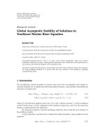
The results of system simulation (13) are shown in figure 1, showing the convergent
states of the system with inputs sin(𝑡) (figure 1a) and 1(𝑡) (figure 1b).
Remarks:
- The initial states of the system are [𝑒(𝑡) 𝑔(𝑡)]T = [1.5 0.5]T.
- Simulation is performed after 20𝑠 the states of the system converge to 0.
- With different inputs, system (13) is asymptotically stable.
- The simulation results are consistent with the theoretical basis.

126 Vu Quoc Huy, “Asymptotic stability of dynamical systems with Barbalat’s … Lyapunov function.”


𝑔(𝑡)

𝑔(𝑡)


Research

𝑒(𝑡)

𝑒(𝑡)

a) Convergent states with 𝜔(𝑡) = 𝑠𝑖𝑛(𝑡).
b) Convergent states with 𝜔(𝑡) = 1(𝑡).
Figure 1. The convergent states of the system with different inputs.
3.2. Analysis of asymptotic stability of a drive control system
3.2.1. Theoretical analysis
Consider a drive control system with the dynamical equation described in (19).
(19)
𝐽𝜃̈(𝑡) = −𝑓(𝜃, 𝑡) + 𝑏𝑢(𝑡)
Tracking angle error and its derivative:
𝑒(𝑡) = 𝜃𝑑 (𝑡) − 𝜃(𝑡)
𝜃̇ (𝑡) = 𝜃̇𝑑 (𝑡) − 𝑒̇ (𝑡)
{
⇒
{
(20)
𝑒̇ (𝑡) = 𝜃̇𝑑 (𝑡) − 𝜃̇(𝑡)
𝜃̈ (𝑡) = 𝜃̈𝑑 (𝑡) − 𝑒̈ (𝑡)
Where: 𝜃 is the actual angle.
𝑓(𝜃, 𝜃̇, 𝑡) = 𝑎𝜃̇ is the term depends on speed angle with vicious coefficient 𝑎.
𝑢 is the control signal.
𝑏 is the control matrix.
𝐽 is the inertial moment of the system.
𝜃𝑑 is the desired angle.

Reform (19) under the tracking error equation by substituting (20) into (19):
𝐽(𝜃̈𝑑 − 𝑒̈ ) = −𝑎(𝜃̇𝑑 − 𝑒̇ ) + 𝑏𝑢
(21)
̈
̇
(22)
𝐽𝑒̈ + 𝑎𝑒̇ + 𝑏𝑢 − (𝐽𝜃𝑑 + 𝑎𝜃𝑑 ) = 0
Set:
(23)
𝑥1 = 𝑒(𝑡); 𝑥2 = 𝑒̇ (𝑡)
Without loss of generality, for simplicity in mathematical representation, consider 𝐽 =
1 𝑘𝑔𝑚2 then the system (22), (23) is reformed as the state equation (24):
𝑥̇ 1 = 𝑥2
{
(24)
𝑥̇ 2 = −𝑎𝑥2 − 𝑏𝑢 + (𝜃̈𝑑 + 𝑎𝜃̇𝑑 )
Choose the autonomous system (25) to be the sliding surface for system (24):
(25)
𝑆 = 𝜆𝑥1 + 𝑥2 = 0, 𝜆 > 0
Suppose we have synthesized the controller 𝑢 such that the derivative of 𝑆 has the
form (26):

Journal of Military Science and Technology, Special issue No.6, 12- 2022

127


Computer science and Control engineering

𝑆̇ = −𝜀sign(𝑆) − 𝑘𝑆; 𝜀, 𝑘 > 0

To analyze the asymptotical stability of the system, select the Lyapunov 𝑉.
1
𝑉 = 𝑆2
2
𝑉̇ = 𝑆𝑆̇
Substitute (26) into (28):
𝑉̇ = −𝜀|𝑆| − 𝑘|𝑆|2 ≤ 0 ∀𝑆

(26)

(27)
(28)
(29)

From (29), according to Lagrange’s theorem, 𝑉(𝑡) is a decreasing function
(monotonical decreasing) with ∀𝑆 ≠ 0, which means that when comparing 𝑉(𝑡) at the
initial time 𝑡 = 0 and later time 𝑡 > 0, there’s always 𝑉(𝑡) ≤ 𝑉(0), means that 𝑉(𝑡) is
bounded. Since 𝑉(𝑡) is bounded, so according to (12), 𝑆 is also bounded.
Because 𝑉̇ (𝑡) is semi-negative, so it is impossible to conclude |𝑆| → 0. To apply
Barbalat’s lemma, we need to calculate the second derivative of 𝑉(𝑡) and make sure that
𝑉̈ (𝑡) is bounded to be possible to conclude 𝑉̇ (𝑡) is uniformly continuous.
Indeed, from (29), calculate the second derivative of 𝑉(𝑡):
𝑉̈ = −𝜀|𝑆̇| − 2𝑘𝑆𝑆̇
(30)
Substitute (26) into (30):
𝑉̈ = −𝜀|𝜀sign(𝑆) + 𝑘𝑆| + 2𝜀𝑘|𝑆| + 2𝑘 2 𝑆 2

(31)

Formula (31) shows that 𝑉̈ is the function of bounded terms 𝑆, therefore 𝑉̈ is bounded

and deduces 𝑉̇ is uniformly continuous.
Barbalat’s lemma allows us to conclude:
(32)
𝑉̇ = −𝜀|𝑆| − 𝑘|𝑆|2 → 0
Therefore |𝑆| → 0.
Thus, if the control law ensures the derivative of 𝑆 has the form (26), the control
system is asymptotically stable. Furthermore, if the control law guarantees for 𝑆 → 0 in
finite time, then at the time 𝑡0 when the state of the system falls on the sliding surface,
the equation 𝑆 = 0 exists.
From (23) to have:
𝑆 = 𝜆𝑥1 + 𝑥2 = 0 ⇒ 𝜆𝑥1 = −𝑥2 ⇔ 𝜆𝑥1 = −𝑥̇ 1
1
(33)
⇒ ln|𝑥1 | = − 𝑡 + 𝐶,
𝐶 = 𝑐𝑜𝑛𝑠𝑡
𝜆
Suppose the system states at the time on the sliding surface: 𝑥1𝑠 |𝑡=𝑡0 = 𝑥1𝑠 (𝑡0 ), one has:
1
(34)
𝐶 = ln|𝑥1𝑠 (𝑡0 ) | + 𝑡0
𝜆
Substitute (34) into (33) to have:
1
(35)
ln|𝑥1 | = − 𝑡 + ln|𝑥1𝑠 (𝑡0 )|
𝜆
1
(36)
𝑥1 = 𝑥1𝑠 (𝑡0 )𝑒 −𝜆(𝑡−𝑡0 )


128 Vu Quoc Huy, “Asymptotic stability of dynamical systems with Barbalat’s … Lyapunov function.”


Research

𝑥1𝑠 (𝑡0 ) −1(𝑡−𝑡0)
𝑒 𝜆
𝜆
Since 𝜆 > 0 so, from (36) shows that 𝑥1 , 𝑥2 → 0 when 𝑡 → ∞.
3.2.2. A simulation example
Suppose the parameters of the system (24) as (37) [9]:
𝑥̇ 1 = 𝑥2
{
𝑥̇ 2 = −25𝑥2 − 133𝑢𝑣 + (𝜃̈𝑑 + 25𝜃̇𝑑 )
𝑥2 = −

(37)

Assuming initial angular position and angular speed:
𝜃𝑑 (0) = −0.5 𝑟𝑎𝑑; 𝜃̇𝑑 (0) = −0.5 𝑟𝑎𝑑/𝑠

(38)

With the step input desired angle 𝜃𝑑 (𝑡) = 1(𝑡), the initial system states are:
[𝑥1 𝑥2 ]𝑇 = [1.5 0.5]𝑇
Select the sliding surface (40):
𝑆 = 15𝑥1 + 𝑥2
The approaching law to sliding surface 𝑆 = 0:

(39)

(40)

𝑆̇ = −70sgn(15𝑥1 + 𝑥2 ) − 20(15𝑥1 + 𝑥2 )

(41)

The controller is synthesized according to [9]:
1
[20(15𝑥1 + 𝑥2 ) + 70sgn(15𝑥1 + 𝑥2 ) − 10𝑥2 ]
133

(42)

x2 (rad/s)

Sliding function S

𝑢=

x1 (rad)

Time (s)

a) Convergence of 𝑆 to 0.

b) Convergence of the system states to 0.

Figure 2. Sliding surface and convergent states of the tracking drive system.
Remarks:
- Figure 2 shows that in the case of a system using control laws, the sliding surface

𝑆 = 0 (an intermediate autonomous system in the control system) always exists, and the
system states converge to 0.
- The two examples above are typical cases illustrating the application of Barbalat’s
lemma when proving the asymptotic stability of a dynamical system according to the
Lyapunov stability principle.

Journal of Military Science and Technology, Special issue No.6, 12- 2022

129


Computer science and Control engineering

4. CONCLUSION
The asymptotic stability of a non-autonomous dynamical system is considered based
on the Lyapunov stability theory. The bounded property of a form of the Lyapunov
function has been confirmed by Lagrange’s theorem, which serves as the basis for the
application of Barbalat’s lemma, ensuring the asymptotic stability of the system. The
article has explained and clarified the application of Barbalat’s lemma and Lagrange’s
theorem; through 2 typical examples to confirm the solid mathematical basis in
analyzing the asymptotic stability of a dynamical system. Of course, the main difficulty
in using Barbalat’s lemma to examine the stability of dynamical systems is choosing the
appropriate Lyapunov function.
REFERENCES
[1]. Hung JY, Gao W, Hung JC, “Variable Structure Control: A Survey”, IEEE Transaction on
Industrial Electronics, Vol. 40, No. 1, pp. 2-22, (1993).
[2]. Ying-Ying M., L. Yun-Gang, “Barbalat lemma and its application in analysis of system
stability”, Journal of Shandong University (Engineering Science), 37(1), 51–56, (2007).
[3]. Slotine and Li, “Applied nonlinear control”, Prentice Hall, pp. 125, (1991).
[4]. Khalil, H. K., “Nonlinear systems”, Englewood Cliffs, NJ: Prentice Hall, (1996).

[5]. Hou, M., Duan, G., & Guo, M., “New versions of Barbalat’s lemma with applications”,
Journal of Control Theory, (2010).
[6]. Narendra, K. S., & Annaswamy, M., “Stable adaptive systems”, New York, NY: Dover
Publications Inc, (2005).
[7]. Yu, X., & Wu, Z., “Corrections to Stochastic Barbalats lemma and its applications”, IEEE
Transactions on Automatic Control, 59, 1386–1390, (2014).
[8]. Nguyễn Ngọc Cư, Lê Huy Đạm, Trịnh Danh Đằng, Trần Thanh Sơn, “Giải tích 1”, Nhà xuất
bản ĐHQG, Hà Nội, (2004).
[9]. Nguyen Thi Thu Thao, Vu Quoc Huy, “Sliding mode control with exponent sliding surfacereaching law in the tracking drive systems using synchronous servo at torque-position
mode”, Journal of Military Science and Technology, No. 80, pp. 31-38, (2022).

TĨM TẮT
Tính ổn định tiệm cận của hệ thống động với bổ đề Barbalat và hàm Lyapnunov
Bài báo diễn giải, kết hợp ứng dụng bổ đề Barbalat, hàm Lyapunov và định lý
Lagrange nhằm đảm bảo tốn học vững chắc trong việc phân tích tính ổn định
tiệm cận của một hệ thống động. Kết quả nghiên cứu được minh họa và mô phỏng
bằng một số ví dụ trực quan, cho cả hệ thống động học khơng điều khiển và hệ
thống động lực học có điều khiển.
Từ khoá: Bổ đề Barbalat; Hàm Lyapunov; Định lý Lagrange; Ổn định tiệm cận; Hệ không tự trị.

130 Vu Quoc Huy, “Asymptotic stability of dynamical systems with Barbalat’s … Lyapunov function.”