An Estimated Replacement Approach for Stable Control of a Class of Nonlinear Systems with Unknown Functions of States
Bạn đang xem bản rút gọn của tài liệu. Xem và tải ngay bản đầy đủ của tài liệu tại đây (299.26 KB, 6 trang )
Proceedings of the World Congress on Engineering and Computer Science 2007
WCECS 2007, October 24-26, 2007, San Francisco, USA
An Estimated Replacement Approach for Stable
Control of a Class of Nonlinear Systems with
Unknown Functions of States
Nguyen Duy Hung and Nguyen Thi Huong Lan, VIELINA
Abstract—In this paper, we propose an approach for stable
control of a class of nonlinear systems, which can be expressed in a
state-feedback linearizable form with unknown nonlinear
functions of states. The idea is to replace the unknown functions
with estimated (not need to be accurate) functions and to use a
universal approximator to compensate for the error caused by the
replacement. For achieving a stable controller with a continuous
control signal, a bisigmoid function based compensator is used
and studied. In addition, the paper also deals with the control
problem of input constraints and the way to examine this subject.
In general, the unknown function(s) g ( x) or g (x), f (x) is/are
approximated by adjustable function approximator(s)
g (x, θ g ) or g (x, θ g ), f (x, θ f ) respectively, where θ g , θ f
are weights or parameter vectors. As the aim is to design a
stable adaptive controller with suitable adaptation law to reduce
uncertainties in each case, g must be other than zero on the
Index Terms—nonlinear control, unknown functions, estimated
replacement, universal approximators.
domain Ω x to avoid singularities at g = 0 during adaptation.
To deal with such a problem a parameter projection method is
employed ([10], [11]), but this situation can also be avoided
when using techniques presented in some schemes, such as a
modified Lyapunov function ([7]) or a modified term ([8]).
I. PROBLEM FORMULATION
II. AN ESTIMATED REPLACEMENT APPROACH
Consider a SISO nonlinear system in its full state-feedback
linearizable form [3]
x1 = x2
Suppose that, from a knowledge of the system we can find
out continuous and bounded functions f (x) and g (x) > 0
xn −1 = xn
(1)
xn = f ( x ) + g ( x )u
Δ dxn (x, u ) ≤ W holds for all x ∈ Ω x , u ∈ Ωu where
Δ dxn ( x, u ) = f ( x ) − f ( x ) + ( g ( x ) − g ( x ) ) u
y = x1
where x = [ x1 , x2 ,…, xn ] ∈ Ω x ⊂ ℜn is a state vector,
T
u(t ) ∈ Ωu ⊂ ℜ is an input ( Ω x , Ωu are compact sets),
y (t ) ∈ℜ is an output, and f ( x ) ∈ℜ , g ( x ) ∈ℜ are unknown,
but continuous and bounded functions. The control objective is
to design a locally stable controller for tracking a reference
trajectory r (t ) ∈ ℜ with bounded error. Because g (x) can not
be zero, without loss of generality, we can assume that
g (x) > 0 for all x ∈ Ω x . Additionally, it also assumes that x
are measurable whereas r (t ) and its derivatives up to the n-th
one are bounded and known.
For the given control problem, many adaptive designs have
been developed as shown in [7]-[12] and the references therein.
Manuscript received July 6, 2007. VIELINA is the Vietnam Institute of
Electronics, Informatics, and Automation. Address: 156A Quan Thanh St.,
Hanoi, Vietnam.
The authors are with the Center of Automation and Control, VIELINA
(e-mail: ).
ISBN:978-988-98671-6-4
such that if we replace f (x) , g (x) in (1) with f (x) , g ( x )
respectively, we can approximate xn with bounded error, i.e.,
= Δ f ( x ) + Δ g ( x )u
and W > 0 is a bounded constant. Based on a method mainly
derived from [3], let us define an error system
E (t , x ) = k T e
(2)
where e = x − r , rT = ⎡ r , r , … , r ( n −1) ⎤ , k T = ⎡⎣k1 , … , kn −1 ,1⎤⎦
⎣
⎦
with s n −1 + kn −1s n −2 + … + k1 is a Hurwitz polynomial.
In the sense of performance analysis, the error system
provides a quantitative measure of the closed-loop system
performance. Hence, once the system dynamics are used with
the definition of the error system to define the error dynamics, a
Lyapunov candidate V ( E ) is then used to provide a scalar
measurement of the error system. In addition, in terms of
boundedness, the error system and the Lyapunov candidate are
also chosen such that bounding V will place bounds on the
error system E and the system states x too.
To focus on the main idea of this paper, we accept without
WCECS 2007
Proceedings of the World Congress on Engineering and Computer Science 2007
WCECS 2007, October 24-26, 2007, San Francisco, USA
proof that (2) satisfies the error system assumption (see
Appendix A). Additionally, for the time being, we ignore the
local stabilization case and do not take the state and input
bounding conditions into consideration. Thus if we denote
k TE = [ k1 ,…, kn −1 ] and dTE = ⎡ x1 − r, x2 − r ,…, xn −1 − r ( n −2) ⎤ ,
⎣
⎦
the
error
system
(2)
can
be
rewritten
as
)
(
E (t , x ) = k TE d E + xn − r ( n −1) and its time derivative (i.e., the
error dynamic) becomes
E = k TE d E + xn − r ( n)
(3)
= k TE d E − Δ dxn − r ( n) + f + gu.
u=u= g
where η > 0
V (E) =
1
2
(
−k TE d E
and
+r
(n)
− f −η E
consider
the
)
Lyapunov
(4)
candidate
2
E , then the time derivative of the Lyapunov
function along the solution of the error dynamic (3) is bounded
by
≤ −ηV − 12 η E 2 + W E
= −ηV +
2
W2
1
−
(W − η E )
2η 2η
≤ −ηV +
W2
.
2η
V≤
W
2η
2
⇒ E ≤
and lim VH =
t →∞
η2
W2
2η 2
enough, the closed-loop system performance depends only on
the error bound W in approximating xn without considering
about how large the individual approximation errors Δ f (x)
and Δ g (x) in replacing the unknown functions are. This
means that we can replace the unknown functions with
preferred estimated functions at our convenience provided that
the approximation error Δ dxn is bounded by W .
Theorem 1: The state-feedback control law (5) ensures that
the solution of the error dynamic (3) is uniformly ultimately
bounded by (6) if there exist continuous and bounded functions
f (x) and g (x) > 0 such that Δ dxn (x, u ) ≤ W holds for all
x ∈ Ω x , u ∈ Ωu where W > 0 is a known bounded constant.
such that
(7)
∂V
E ≤ −γ 3 ( E )
∂E
for ∀ E ≥ R and t ≥ 0 with knowing that V ( E ) is
V (E) =
0
− t
= VH
(1 − e η ) + E e η
− t
continuously differentiable on E ≥ R .
Choosing γ 1 ( E ) = γ 2 ( E ) = V ( E ) =
(1 − e η ) + V e η
W2
Remark 3: From (6), we see that if we choose E0 small
γ1 ( E ) ≤ V ( E ) ≤ γ 2 ( E )
W2
, we obtain
2η
− t
for all t ≥ 0 .
[0, ∞ )
Let V0 and E0 denote the V and E at t = 0 , thus
according to the lemma of ultimate bound (Appendix B) with
2
2 − t
0
= V∞ , lim EH =
t →∞
W
η
V ( E ) ≤ −ηV +
= EH
= −εηγ 1 ( E ) − (1 − ε )ηV +
V ( E ) ≤ −γ 3 ( E )
+ η E = η e and the control law (4) can be
then
formulated as
T
(
)
(5)
Remark 2: If V0 ≤ V ( E∞ ) then 0 ≤ V ≤ V ( E∞ ) for all
t ≥ 0 since V is positive definite so that it can not grow
greater than V ( E∞ ) . Furthermore, in the case of V0 > V ( E∞ )
we have V ≤ 0 until V ≤ V ( E∞ ) , thus we find
ISBN:978-988-98671-6-4
E
2
we have
W2
2η
for ε satisfying 0 < ε < 1 . Let γ 3 ( E ) = εηγ 1 ( E ) we see that
= E∞ .
Remark 1: If we denote η = ⎡⎣η k1 , k1 + η k2 , … , kn −1 + η ⎤⎦
u = u = g −1 r ( n ) − ηT e − f
1
2
W2
2η
if
and
T
k TE d E
(6)
Proof: According to a theorem of condition for uniform
ultimate boundedness ([2]), in proving Theorem 1 we wish to
find some γ 1 ( E ), γ 2 ( E ) ∈ K ∞ and γ 3 ( E ) ∈ K defined on
V = EE = −η E 2 − Δ dxn E
m1 = η and m2 =
)
Above results lead to the state of the following theorem.
In terms of feedback linearization, use the control law
−1
(
0 ≤ V ≤ max (V0 , V ( E∞ ) ) ⇒ E ≤ max E0 , E∞
equivalently, E ≥
only
if V ≥
W2
2(1 − ε )η 2
,
or
W
= R . As the chosen functions
1− ε η
fulfill requirement (7), Theorem 1 is thus proved.
Theorem 1 shows that it is possible to define (static)
stabilizing controllers by applying the method of estimated
replacement if we could find substitution functions satisfying
the bounding condition over a valid region. But a problem
arises when W is large, since though the error system bound
may be decreased by choosing η large, the control signal may
WCECS 2007
Proceedings of the World Congress on Engineering and Computer Science 2007
WCECS 2007, October 24-26, 2007, San Francisco, USA
increase in amplitude and may start to oscillate. To dealing with
such a problem, the usual approach is to compensate for error
effects caused by the replacement. For this purpose, a number
of techniques, such as nonlinear damping and dynamic
normalization ([3]) may be used. In this sense, here we propose
a method which comes from the notion that if we can
approximate Δ dxn (x, u ) with sufficiently small error, it is
possible to include an additional stabilizing component to
increase the robustness of the closed-loop system.
Because Δ dxn (x, u ) is a continuous and bounded function
defined on compact sets, it can be approximated by a universal
approximator (such as a fuzzy system or a neural network) with
arbitrary accuracy. Therefore by assumption that there are data
available for tuning of an approximator to match certain
condition, we can use it as a compensation component to form a
robust state-feedback control law. This subject will be studied
in more detail later in this paper. Now, before turning to
developing a stable controller for making the closed-loop
system more robust to system uncertainties, we will investigate
some mathematical base.
or equivalently
− x + ( ρ + 1) = −( ρ + 1)e − x .
This equation is in form of x + b = ae x where a ≠ 0 , thus
according to [13] it has the single root, equal to −b − w( −ae −b )
where w( x ) is the Lambert w-function (Note that the Lambert
w-function is the inverse function of x = w( x )e w( x ) ). The
substitution for a = −( ρ + 1) and b = ρ + 1 leads to the
solution of (10), afterward denote as x0 = ρ + 1 + w(p) where
p( ρ ) = ( ρ + 1)e −( ρ +1) .
Because of
dp
= − ρ (2 + ρ )e −( ρ +1) < 0 , p is decreasing
dρ
)
for ρ ∈ ( 0,1] , therefore p(1) ≤ p( ρ ) < p(0) or p ∈ ⎡ 2 e2 ,1 e .
⎣
Consequently μ x ( ρ , x ) has the unique extremum at x0 and if
we denote μ 0 = μ x ( ρ , x0 ) then
μ 0 = ( ρ + 1)e−2 x0 + 2( ρ − x0 )e− x0 + ρ − 1
⎛ 1 ⎞
= ( ρ + 1)e−2( ρ +1) ⎜
⎟
⎝ e w(p) ⎠
III. MATHEMATICAL BASE
Define a real-valued scalar function
μ E ( ρ , κ , E ) = E ( ρ − sgn( E ) bsig(κ , E ) )
(10)
2
+2 [ ρ − ( ρ + 1) − w(p)] e−( ρ +1)
(8)
where 0 < ρ ≤ 1 , κ > 0 are parameters, E ∈ℜ is a variable,
1
e
w(p)
+ ρ −1
2
Lemma 1. The function (8) reaches its positive maximum
value of μ E _ max ( ρ , κ ) = μ E ( ρ , κ , ± Em ) at ± Em where
⎡
⎤
w(p)
= ( ρ + 1)e −2( ρ +1) ⎢
⎥
⎢⎣ ( ρ + 1)e−( ρ +1) ⎥⎦
w(p)
−2 (1 + w(p) ) e −( ρ +1)
+ ρ −1
( ρ + 1)e−( ρ +1)
x = κ Em is the unique solution of the equation
=
sgn( E ) is the sign function, and bsig(κ , E ) = 2 /(1 + e −κ E ) − 1
is bisigmoidal.
μ x ( ρ , x ) = ( ρ + 1)e −2 x + 2( ρ − x )e − x + ρ − 1 = 0
(9)
Proof: Because (8) is an even function, thus we can take only
the case E ≥ 0 , i.e., μ E + ( ρ , κ , E ) = E ( ρ − bsig(κ , E ) ) into
account. It follows that the derivative of μ E + with respect to
E can be calculated as
( ρ + 1)e−2 x + 2( ρ − x)e− x + ρ − 1 μ x ( ρ , x)
d
=
μE+ =
2
2
dE
−x
1+ e
1 + e− x
(
)
(
)
where x = κ E ≥ 0 . Obviously, μ E+ has its extremum at
xm = κ Em if satisfies μ x ( ρ , κ Em ) = 0 . Next we will show
that, x = xm is the unique solution of (9) and μ E _ max ( ρ , κ ) is
a positive maximum.
Take the derivative of μ x ( ρ , x ) with respect to x , we
obtain
d
μ x ( ρ , x ) = 2e − x ⎡ x − ( ρ + 1) − ( ρ + 1)e − x ⎤ .
⎦
⎣
dx
d
μ x ( ρ , x) = 0
For studying μ x ( ρ , x ) , solve the equation
dx
ISBN:978-988-98671-6-4
=
w 2 (p)
w(p)
− 2 (1 + w(p) )
+ ρ −1
ρ +1
ρ +1
ρ 2 − ( w(p) + 1)
ρ +1
2
.
Since the Lambert w-function is strictly increasing on
[− 1 e , ∞ )
we get w(2 e 2 ) ≤ w(p) < w(1 e) , thus x0 > 1 and
μ 0 < 0 for all ρ ∈ ( 0,1] . In addition μ x ( ρ , 0) = 4 ρ > 0 and
μ x ( ρ , ∞) = ρ − 1 ≤ 0 so that the graph of μ x ( ρ , x ) cuts the
x-axis only at xm ∈ ( 0, x0 ) as well as the extremum μ 0 is the
minimum of μ x ( ρ , x ) .
Note that
μ ( ρ , x)
d
μE+ = x
, we can infer that μ E+
2
dE
1 + e− x
(
)
reaches its maximum value of μ E + ( ρ , κ , Em ) = μ E _ max ( ρ , κ )
at Em =
xm
κ
> 0 and as μ E + ( ρ , κ , 0) = 0 , the unique
maximum is positive. This proves Lemma 1.
For a better understanding of Lemma 1, Fig. 1 shows graphs
WCECS 2007
Proceedings of the World Congress on Engineering and Computer Science 2007
WCECS 2007, October 24-26, 2007, San Francisco, USA
of (8) in cases of κ = 5 and κ = 10 with ρ = 0.5, 0.9,1 in each
example whereas Fig. 2 illustrates the graph of Em ( ρ , κ ) and
μ E _ max ( ρ , κ ) with respect to ρ and κ in the case of κ = 1
and ρ = 1 respectively.
κ =5
κ = 10
0.06
0.1114
0.0557
0.0879
0.0440
Δ dxn (x, u ) = f (x) − f (x) + ( g (x) − g (x) ) u ≤ W
for all x ∈ Ω x , u ∈ Ωu where W > W . We will search for a
solution to cope with this problem.
As mentioned above, the error function Δ dxn can be
approximated by the universal approximator within a compact
Fig. 1. Graphs of μ E ( ρ , κ , E )
0.12
enough). However the estimated functions available for use
only guarantee that
set, which hereafter we denote as FΔ (x, u , θ) where θ ∈ ℜ p is
an adjustable parameter vector and FΔ (x, u, θ) ∈ ℜ . Right now
0.08
μE
μE
←ρ = 1
0.04
0.0256
tunable parameters θ . Assume that WΔ > 0 be the known
approximation error bounding constant, which satisfies
FΔ (x, u, θ) − Δ dxn (x, u ) ≤ WΔ
0.02
0
← ρ = 0.9
0
← ρ = 0.5
-0.5
0
E
0.5
← ρ = 0.5
1
-0.02
-0.5
-0.25
0
E
0.25
0.5
Fig. 2. Graphs of Em ( ρ , κ ) and μ E _ max ( ρ , κ )
κ =1
ρ =1
1.4
0.4
1.2785
1.2
1.0769
0.3
0.2557
0.8
← Em
← Em
0.2
0.6
0.5569
0.5229
0.1278
0.1114
0.1
0.4396
0.4
← μE_max
0.2
← μE_max
0.0557
0.1278
0.2
0.4 0.5 0.6
0.8 0.9 1
0
0
for all x ∈ Ω x , u ∈ Ωu and θ ∈ℜ p is the best known
parameter vector available from adjusting the parameters of the
approximator. Therefore the problem for approximating xn
with error bound W can be considered as the problem for
approximating Δ dxn with error bound WΔ . Thus, we can avoid
the difficulty of dealing with choosing estimated functions
correctly by working with a proper approximator to
compensate for the effect of the replacement error. But one
must determine how small WΔ must be to achieve the desired
closed-loop system performance.
In order to solve this problem, now we introduce the
compensation component defined as
F ( x, u, θ)
uc = − Δ
bsig κ , EFΔ ( x, u, θ)
(12)
ρ g (x)
where ρ , κ are constants satisfying 0 < ρ ≤ 1 , κ > 0 and u
is specified by (5). Then adding the component (12) together
with the state-feedback control law (5) forms the new control
law
(13)
u = u + uc
and consequently the following theorem is the extension of
Theorem 1 to this case.
(
1
0
0
(11)
0.0128
← ρ = 0.9
-0.04
-1
let FΔ (x, u , θ) represent a neural network or fuzzy system with
0.04
←ρ = 1
5
ρ
10
15
20
κ
)
Theorem 2: If there exist an approximator FΔ (x, u , θ) and a
parameter vector θ such that FΔ (x, u , θ) can approximate
IV. CONTROLLER DESIGN
Recall from previous studies that we are going to develop a
stable controller in the proposed approach called estimated
replacement. The main concept in this approach is to seek
estimated functions fitting the bounding requirement and to use
a compensation technique to make the controller robust to
uncertainties. The later problem can be considered in this
section as follows.
Suppose that we have to design a controller for the tracking
problem with the aim to keep the error system bounded by
W
E∞ =
(it is assumed that E0 can be selected small
η
ISBN:978-988-98671-6-4
Δ dxn (x, u ) with error bounded by WΔ satisfying
0 < WΔ ≤ W 2 −
2η
ρ
μ E _ max ( ρ , κ )
(14)
for all x ∈ Ω x , u ∈ Ωu where 0 < ρ ≤ 1 , κ > 0 and η > 0
then the state-feedback control law (13) ensures that the
solution of the error dynamic (3) is uniformly ultimately
bounded by (6).
Proof:
For simplicity, denote FΔ = FΔ (x, u, θ) , FΔ = FΔ ( x, u, θ)
WCECS 2007
Proceedings of the World Congress on Engineering and Computer Science 2007
WCECS 2007, October 24-26, 2007, San Francisco, USA
then from E = −η E + g (x )uc − Δ dxn ( x, u ) we have
the system error is uniformly ultimately bounded by (6) while
satisfying input constraints u ∈ Ωu where Ωu is defined as
V = −η E 2 + Eg ( x )uc − E Δ dxn ( x, u )
≤ −η E 2 −
≤ −η E 2 +
1
ρ
(15) if uM >
EFΔ bsig(κ , EFΔ ) + E Δ dxn
1
ρ
(
)
E ρ Δ dxn − FΔ sign( E ) bsig(κ , EFΔ ) .
Since sgn( E ) sgn( FΔ ) = sgn( EFΔ ) and Δ dxn ≤ FΔ + WΔ
Proof: By assumption, the estimated functions f (x) , g (x)
are locally Lipschitz continuous, therefore we can find
constants K f , K g such that
so we obtain
V ≤ −η E + E WΔ +
2
= −η E + E WΔ +
2
= −ηV
W2
+ Δ
2η
−
E
ρ
ρ
( ρ − sgn( EFΔ ) bsig(κ , EFΔ ) )
r ( n) − ηT e − f (x) −
u =
2
1
(WΔ − η E ) + ρ1 μ E (κ , EFΔ )
2η
μ E (ρ ,κ , E )
is
defined
as
in
(8)
E ∈ℜ as stated in Lemma 1.
Clearly, to have the error system bounded by (6), we need
2
W
, hence it follows that the requirement (14)
2η
holds. Notice that because WΔ > 0 , we must choose ρ , κ and
η such that
1
ρ
(
FΔ bsig κ , EFΔ
)
g ( x)
=
r ( n) − ηT e − f (e + r ) + f (r ) − f (r ) FΔ bsig(κ , EFΔ )
−
ρ g (r )
g (r )
×
g (r )
g (e + r )
and
μ E ( ρ , κ , E ) ≤ μ E _ max ( ρ , κ ) for all 0 < ρ ≤ 1 , κ > 0 and
V ≤ −ηV +
g ( x) − g ( x) ≤ K g x − x
for ∀x, x ∈ Ω x . From (13) and note that x = e + r we have
W2 1
≤ −ηV + Δ + μ E _ max ( ρ , κ )
2η ρ
where
f ( x) − f ( x) ≤ K f x − x
( ρ FΔ − FΔ sgn( E ) bsig(κ , EFΔ ) )
EFΔ
W + WΔ
and the condition (17) holds.
ρ gL
2η
μ
(ρ , κ ) < W 2 .
ρ E _ max
Then similar to the proof of Theorem 1, we come to that the
new control law (13) makes the solution of the error system (3)
uniformly ultimately bounded by (6). This proves Theorem 2.
V. INPUT CONSTRAINTS ANALYSIS
Up to this point we have not taken a state boundedness and
input constraints into account. However, for state boundedness,
we can examine it using the error system boundedness. In this
section, we only consider the case of input constraints. Notice
that the original work on stabilization and tracking of feedback
linearizable systems under input constraints in which we have
utilized its concepts can be reviewed in [6].
The problem of input constraints can be stated here as how
to select parameters (if they exist) for the control design so that
the control input (13) always remains in a valid region Ωu ,
which is defined as
Ωu = {u ∈ ℜ : u ≤ uM }
(15)
where uM is positive bounded constant. Additionally, it
assumes 0 < g L ≤ g (x) and f (x) , g (x) can be chosen so that
they are locally Lipschitz in x .
Since FΔ ≤ W + WΔ and recall that W > W , we get
⎛ r ( n ) − f (r )
ηT e
f (r ) − f (e + r )
u ≤⎜
+
+
⎜
g (r )
g (r )
g (r )
⎝
F bsig(κ , EFΔ ) ⎞
g (e + r ) − g (r )
+ Δ
⎟× 1−
⎟
g (e + r )
ρ g (r )
⎠
⎛ r ( n ) − f (r ) K e
FΔ
η e
f
≤⎜
+
+
+
⎜
g (r )
g (r )
g (r ) ρ g (r )
⎝
⎞⎛
Kg e
⎟ ⎜1 +
⎟⎜
g (e + r )
⎠⎝
⎞
⎟
⎟
⎠
⎛ r ( n ) − f (r )
e W + WΔ ⎞ ⎛
e ⎞
⎟ ⎜1 + K g
≤⎜
+ η +Kf
+
⎟
⎜
⎜
g (r )
gL
ρ gL ⎟ ⎝
g L ⎟⎠
⎝
⎠
In order to have the control input remain in Ωu , we need
(
r ( n) − f (r )
≤u =
g (r )
)
uM
1+ Kg
e
(
− η +Kf
)g
e
L
−
W + WΔ
. (16)
ρ gL
gL
In addition, as E = k e ≤ max ( E0 , E∞ ) so we can write
T
(
)
e(t ) ≤ K max E0 , E∞ = eM where eM > 0 . Let’s define
M =
uM
e
1+ Kg M
gL
(
− η +Kf
) gM
e
L
−
W + WΔ
ρ gL
then M ≤ u and we see that if M > 0 then (16) always holds.
To have M > 0 , it requires
Theorem 3: The state-feedback control law (13) ensures that
ISBN:978-988-98671-6-4
WCECS 2007
Proceedings of the World Congress on Engineering and Computer Science 2007
WCECS 2007, October 24-26, 2007, San Francisco, USA
⎛
e ⎞⎛
e
W + WΔ
uM > ⎜ 1 + K g M ⎟ ⎜ η + K f M +
⎜
ρ gL
gL ⎠ ⎝
gL
⎝
(
)
y (t ) → r (t )
⎞
⎟⎟
⎠
2
⎛e ⎞ ⎛
W + WΔ ⎞ eM
⇔ Kg η + K f ⎜ M ⎟ + ⎜ η + K f + Kg
⎟
⎜
ρ g L ⎟⎠ g L
⎝ gL ⎠ ⎝
W + WΔ
+
− uM < 0
ρ gL
The above quadratic inequation is in the form of
e
Az 2 + Bz + C < 0 where z = M > 0 and
gL
(
)
(
)
A = Kg η + K f > 0
B = η + K f + Kg
C=
W + WΔ
− uM .
ρ gL
W + WΔ
so that it has a positive one. It
need C < 0 , i.e., uM >
ρ gL
K
− B + B 2 − 4 AC
max ( E0 , E∞ ) < z2 =
gL
2A
satisfies
APPENDIX B
A ULTIMATE BOUND STUDY (LEMMA 2.1 IN [3])
If
V (t , E) : ℜ+ × ℜn → ℜ+
is
positive
definite
and
V ≤ − m1V + m2 where m1 > 0 and m2 ≥ 0 are bounded
[1]
[2]
[3]
[4]
[5]
[6]
and therefore we must choose (if it exists)
)
E(t , x )
to e ∈ ℜ+ for each fixed t .
follows that
(
function
m2 ⎛
m ⎞
+ ⎜ V (0) − 2 ⎟ e − m1t for all t .
m1 ⎝
m1 ⎠
REFERENCES
the solution of the quadratic inequation is z1 < z < z2 . Since if
C ≥ 0 , the mentioned polinomial has non-positive roots so we
max E0 , E∞
the
x ≤ ψ x (t , E ) for all t , where ψ x : ℜ+ × ℜ+ → ℜ is bounded
for any bounded E and ψ x (t , e) is nondecreasing with respect
W + WΔ
>0
ρ gL
g
r ( n) − f (r )
< L z2 and
≤M
g (r )
K
that
constants, then V (t , E) ≤
Let z1 < z2 are roots of the polynomial Az 2 + Bz + C then
0< z=
and
[7]
(17)
[8]
for solving the problem of input constraints. (Q.E.D.)
VI. CONCLUSION
In summary, the proposed approach gives a new concept to
design stable controllers for state-feedback linearizable
systems with unknown functions of states. In this way we can
also avoid the problem of singularities mentioned above
because the estimated functions for replacement can be chosen
at our intention and they are known in advance. However the
controller we have developed in this paper is static, that is its
parameters are not adjustable during operation and therefore it
is “less robust” to uncertainties than an adaptive equivalent.
Due to the scope of this topic, we will study adaptive schemes
in another paper. Additionally, achieved results are intended to
be used in real time control systems for industrial applications
in the fields of control of chemical processes, water treatment
control and robot control.
[9]
[10]
[11]
[12]
[13]
Hassan K. Khalil, “Nonlinear Systems”, 3rd ed., Prentice Hall, 2001.
Horacio J. Marquez; “Nonlinear Control Systems: Analysis and Design”,
Wiley Interscience, 2003.
Jeffrey T. Spooner, Mangredi Maggiore, Raúl Ordónez, and Kelvin M.
Passino, “Stable Adaptive Control and Estimation for Nonlinear Systems:
Neural and Fuzzy Approximator Techniques”, Wiley Interscience, 2002.
Jyh-Shing Roger Jang, Chuen-Tsai Sun, and Eiji Mizutani, “Neuro-Fuzzy
and Soft Computing: A Computational Approach to Learning and
Machine Intelligence”, Prentice Hall, 1996.
Nguyen Duy Hung, “Some Neural Network-based Learning Methods and
Problems on Applying in Industrial Control Systems”, Proceedings of 5th
Vietnam Conference on Automation (VICA5), 2002, pp.163–168.
George J. Pappasy, John Lygeros, and Datta N. Godbole, “Stabilization
and Tracking of Feedback Linearizable Systems under Input
Constraints”, Report, Intelligent Machines and Robotics Laboratory,
University of California at Berkeley, 34th CDC, 1995.
T. Zhang, S. S. Ge, and C. C. Hang, “Stable Adaptive Control for a Class
of Nonlinear Systems using a Modified Lyapunov Function", IEEE
Transactions on Automatic Control, vol. 45, no. 1, Jan. 2000.
Jang-Hyun Park, Seong-Hwan Kim, and Chae-Joo Moon, “Adaptive
Fuzzy Controller for the Nonlinear System with Unknown Sign of the
Input Gain", International Journal of Control, Automation, and Systems,
vol. 4, no. 2, Apr. 2006, pp. 178–186.
Hugang Han, Chun-Yi Su, and Yury Stepanenko, “Adaptive Control of a
Class of Nonlinear Systems with Nonlinearly Parameterized Fuzzy
Approximators", IEEE Transactions on Fuzzy Systems, vol. 9, no. 2, Apr.
2001, pp. 315–323.
Jun Nakanishi, Jay A. Farrell, and Stefan Schaal, “Composite adaptive
control with locally weighted statistical learning”, Elsevier Neural
Networks 18, 2005, pp. 71–90.
Jun Nakanishi, Jay A. Farrell, and Stefan Schaal, “Learning Composite
Adaptive Control for a Class of Nonlinear Systems”, Proceedings of the
2004 IEEE International Conference on Robotics & Automation, New
Orleans, LA, pp. 2647–2652.
Shouling He, Konrad Reif, Rolf Unbehauen, “A Neural Approach for
Control of Nonlinear Systems with Feedback Linearization”, IEEE
Transactions on Neural Networks, vol. 9, no. 6, Nov. 1998, pp.
1409–1421.
R.M. Corless, G.H. Gonnet, D.E.G. Hare, and D.J. Jeffrey, “On the
Lambert's W Function”, Technical Report, Advances in Computational
Mathematics, vol 5, 1996, pp. 329–359.
APPENDIX A
AN ERROR SYSTEM ASSUMPTION (ASSUMPTION 6.1 IN [3])
Assume the error system E(t , x ) is such that E = 0 implies
ISBN:978-988-98671-6-4
WCECS 2007