Online optimization of dynamic binding capacity and productivity by model predictive control
Bạn đang xem bản rút gọn của tài liệu. Xem và tải ngay bản đầy đủ của tài liệu tại đây (2.09 MB, 10 trang )
Journal of Chromatography A 1680 (2022) 463420
Contents lists available at ScienceDirect
Journal of Chromatography A
journal homepage: www.elsevier.com/locate/chroma
Online optimization of dynamic binding capacity and productivity by
model predictive control
Touraj Eslami a,b , Martin Steinberger c , Christian Csizmazia a , Alois Jungbauer a,d,∗ ,
Nico Lingg a,d,∗
a
Department of Biotechnology, Institute of Bioprocess Science and Engineering, University of Natural Resources and Life Sciences, Vienna, Muthgasse 18,
Vienna A-1190, Austria
Evon GmbH, Wollsdorf 154, A-8181St., Ruprecht an der Raab, Austria
c
Institute of Automation and Control, Graz University of Technology, Inffeldgasse 21b, Graz A-8010, Austria
d
Austrian Centre of Industrial Biotechnology, Muthgasse 18, Vienna A-1190, Austria
b
a r t i c l e
i n f o
Article history:
Received 13 June 2022
Revised 3 August 2022
Accepted 12 August 2022
Available online 13 August 2022
Keywords:
MPC
Protein A
Linear driving force model
Mechanistic model
Linearization
EKF
a b s t r a c t
In preparative and industrial chromatography, the current viewpoint is that the dynamic binding capacity governs the process economy, and increased dynamic binding capacity and column utilization are
achieved at the expense of productivity. The dynamic binding capacity in chromatography increases with
residence time until it reaches a plateau, whereas productivity has an optimum. Therefore, the loading
step of a chromatographic process is a balancing act between productivity, column utilization, and buffer
consumption. This work presents an online optimization approach for capture chromatography that employs a residence time gradient during the loading step to improve the traditional trade-off between productivity and resin utilization. The approach uses the extended Kalman filter as a soft sensor for product
concentration in the system and a model predictive controller to accomplish online optimization using
the pore diffusion model as a simple mechanistic model. When a soft sensor for the product is placed
before and after the column, the model predictive controller can forecast the optimal condition to maximize productivity and resin utilization. The controller can also account for varying feed concentrations.
This study examined the robustness as the feed concentration varied within a range of 50%. The online optimization was demonstrated with two model systems: purification of a monoclonal antibody by
protein A affinity and lysozyme by cation-exchange chromatography. Using the presented optimization
strategy with a controller saves up to 43% of the buffer and increases the productivity together with
resin utilization in a similar range as a multi-column continuous counter-current loading process.
© 2022 The Author(s). Published by Elsevier B.V.
This is an open access article under the CC BY license ( />
1. Introduction
The prevailing view in preparative and industrial chromatography used to capture a biomolecule from a feedstock is that the
dynamic binding capacity governs the process economy, and increased dynamic binding capacity and column utilization are obtained at the expense of productivity. The dynamic binding capacity in column chromatography increases with increasing residence time until it approaches a plateau, whereas productivity has
an optimum and the column utilization remains low. Therefore,
∗
Corresponding authors at: Department of Biotechnology, Institute of Bioprocess
Science and Engineering, University of Natural Resources and Life Sciences, Vienna,
Muthgasse 18, Vienna A-1190, Austria.
addresses:
(A.
Jungbauer),
(N. Lingg).
the loading step of a chromatographic process requires a balancing
act between productivity, buffer consumption, and resin utilization
[1,2].
The column utilization, productivity, and buffer consumption
are interrelated, and higher column utilization leads to a decrease
in the buffer consumption and productivity [3]. The column utilization and throughput can be optimized by employing strategies of counter-current loading with two or more columns [4–8].
Two main categories of approaches have been studied for optimizing the loading. The first approach, called off-line optimization [9–
11], applies a model-based optimizer to analyze the system’s behavior under different conditions to anticipate the optimal setting,
and the obtained solution is validated experimentally. In the second approach, called online optimization, the system is evaluated
and optimized at each time increment of the process to fulfill the
requirements [12–14]. In this technique, the optimizer uses recent
/>0021-9673/© 2022 The Author(s). Published by Elsevier B.V. This is an open access article under the CC BY license ( />
T. Eslami, M. Steinberger, C. Csizmazia et al.
Journal of Chromatography A 1680 (2022) 463420
measurements and considers all quality constraints and limitations,
then it generates a new control command at each iteration to direct the process to the optimal operating point [15–19].
Ghose et al. [20] used the off-line optimization methodology
and presented a dual-flow-rate strategy for the loading phase. They
discovered that the productivity and resin utilization rate improve
by loading the column at a low residence time and then increasing
it to a higher level. They used a model-based optimizer to evaluate the best switching time between the initial and final residence times. This strategy was expanded recently [11,21] by introducing the multi-flow-rate approach, which applies multiple optimization techniques to successfully improve the productivity while
maintaining resin utilization at a high level. However, it is worth
noting that off-line optimization suffers from reduced robustness
through experimental errors, since it requires a thorough understanding of the dynamics of the system. Additionally, due to the
nature of off-line optimization, the system cannot cope with any
change in the process conditions or any unforeseen disturbance.
Therefore, it may lead to suboptimal results and require iterative
optimization.
Model predictive control (MPC) has become a prominent nonlinear control strategy for online optimization over the last two
decades [15,22–25], and it incorporates concepts from systems
theory, system identification, and optimization [26]. Compared to
commonly employed controllers, such as PID controllers, MPC is an
advanced control method that effectively deals with nonlinearities,
constraints, and uncertainties [12,27]. Moreover, MPC can control
systems that cannot be controlled by conventional feedback controllers [28]. The main goal of MPC is to estimate a future trajectory of the process in the control horizon window to optimize the
system’s future behavior [29]. Complimentary reviews on the advantages and principles of MPC, either linear or nonlinear, are provided by Qin and Bagwell [30–32].
In this work, the MPC controller is built on a computationally
efficient mechanistic model, linear driving force with a pore diffusion model [33], to anticipate the adsorption in the column. Since
this model is highly nonlinear, a linear approximation of the system that corresponds to the general equation with the same behavior is required to enable use within linear MPC. Various methods for linearization can be found in the open literature, including
piecewise linearization [34] to transform the model into multiple
linear parts. Another robust technique is to approximate the linear
format of the system with Taylor expansion at each timing cycle
at a steady-state point [14]. The current work uses successive linearization to approximate the linear model at each operating point.
Toward this end, the extended Kaman filter (EKF) as a soft sensor is used to adaptively estimate the state of the column at the
operating point. The EKF incorporates the information embedded
in the local models into a global description of the nonlinear dynamics and performs state estimation by tracking transition online
[34,35].
We have expanded our previous study [11] by utilizing a MPC
and an EKF to optimize the experiments in batch mode [36–39].
We assessed the performance of the controller by IgG capture with
protein A and lysozyme with cation exchange resin. Our objective
of applying such a strategy is to exploit the maximum benefits of
the process by increasing productivity and resin utilization, regardless of any potential discrepancy between the experimental data
and the corresponding model. The MPC requires an additional sensor for product concentration, which can be a simple UV sensor in
the case of pure material or a soft sensor for crude material [40–
42]. Additionally, we examined the process performance under an
extreme change of concentration at the inlet of the column and in
the presence of white noise. Therefore, at each time step, the controller employs integrated real-time data with the process model
to predict the future dynamics of the system over a finite predic-
tion horizon (N p ). The MPC generates a sequence of control inputs
over a finite control horizon (Nc ) to fulfill the process objectives. It
is worth mentioning that the first element of this sequence will be
applied to the system at each time step. In this way, the controller
requires limited prior knowledge to optimize the process, such as
an approximation of porosity and the adsorption isotherm. There
are advantages when using this strategy; primarily, the system can
cope with the aging of the adsorbent, since the Kalman filter can
provide a good approximation of the system at each timing step.
This will also reduce lab work requirements, since the number of
characterization experiments would be limited in scope [43].
2. Process control via model predictive control
This section presents the mathematical model that describes
the system at each timing cycle. We first describe the basics of the
principle of mass transfer into the column, then we explain the
implementation of the model predictive controller in detail.
2.1. Mathematical modeling of the process
The mass transfer into the column chromatography was predicted using an empirical approximation model known as the linear driving force (LDF) model, given by Eqs. (1) and (2) [33]. This
model considers the movement of solute molecules in the column
due to convection and axial dispersion. Moreover, the overall effective mass transfer coefficient is calculated using pore diffusion
to account for the intraparticle mass transfer resistance, shown by
Eq. (3). The Langmuir isotherm has been used to relate the average
product concentration in the solid phase, q, to the average concentration in the mobile phase, C, as given by Eq. (4).
f ∂C
∂C
∂ 2C
( 1 − εc ) ∂ q
= Dax 2 −
−
∂t
εA ∂ z
ε
∂t
∂z
(1)
∂q
= K q¯ − q
∂t
(2)
K=
15De CF
r 2p qmax
(3)
q¯ =
keq qmax C
1 + keqC
(4)
where t and z are the process time and the position along the
column, respectively; Dax is the axial diffusion; A is the column
cross-sectional area; ε and εc are the total porosity and interparticle porosity, respectively; f is the volumetric flow rate; K is the
overall mass transfer coefficient obtained from the pore diffusion
model; q and q¯ represent the average concentration in the stationary phase and the adsorption isotherm, respectively; De and r p
are the effective diffusivity of the protein solution and the resin
particle radius, respectively; CF is the feed concentration at the inlet of the column; qmax is the maximum column capacity; and keq
is the Langmuir equilibrium constant. It is important to mention
that the pore diffusion is the primary controlling mechanism for
protein liquid chromatography; therefore, the effect of axial dispersion is neglected (De = 0 ) in our work [33]. We successfully implemented this model in our prior work to approximate the general
adsorption of protein with different types of resin [11].
The mass transfer Eq. (1) is a partial differential equation. To
solve this equation numerically, the method of lines (MOL) was
used to discretize the column in the space domain using Ng grid
points [44]. As a result, a set of Ng ordinary differential equations is
generated to approximate the mass transfer into the column. Additionally, the backward Euler method is used to discretize the convection term, given by Eq. (5) [44].
∂ C Ci − Ci−1
=
, i = 1, 2, . . . , Ng−1
∂z
z
2
(5)
T. Eslami, M. Steinberger, C. Csizmazia et al.
Ct (z = 0 ) = CF
∂C
∂z
Journal of Chromatography A 1680 (2022) 463420
dx
= Ac x(t ) + Bc u(t ) + Dc w(t )
dt
(6)
=0
y = Cc x(t )
(7)
(8)
Where z is the distance between two consecutive grid points,
and L is the axial length of the column. Eqs. (6) and (7) describe
the Dirichlet and Neumann boundary conditions at the column’s
inlet and outlet. Eq. (6) states that the concentration at the inlet of
the column is equal to the concentration of the stock solution CF ,
and Eq. (7) indicates that the concentration change at the outlet is
independent of time. Moreover, Eq. (8) is the initial condition and
indicates that the column is empty at the beginning of the process.
This work examines three economic factors in the process, including the resin utilization RU, productivity P r, and buffer consumption BC:
Pr =
BC =
∫V10% (CF − C )dv
DBC10%
= 0
EBC
V (1 − ε ) qmax
DBC10%
tload10% + trest V (1 − ε )
Vbu f f er
DBC10%
(16a)
yNL = yLin + y
(16b)
uNL = uLin + u
(16c)
wNL = wLin + w
(16d)
where xLin , yLin , uLin , and wLin correspond to the values of the internal states, measurement at the outlet, control variable, and concentration at the inlet at the linearizing point, respectively, and x,
y, u, and w are the related variation variables. The nonlinear format of the aforementioned variables is indicated by the subscript
NL. Consequently, based on the Taylor expansion, the linearized
form of the model at each timing cycle can be represented as in
Eqs. (14) and (15).
Ac , Bc , and Dc are the Jacobian matrices of the state function f
(Eq. (12)) with respect to states x, control input u, and the concentration at the inlet CF , respectively. Accordingly, the matrix Cc is
the Jacobian matrix of the output function g (Eq. (12)) with respect
to x.
2.2. Control approach
There are numerous ways to apply a model predictive control
framework to a system with linear and nonlinear equations. This
work uses a discrete-time state-space representation of the model,
which is a well-established technique with MPC [28].
In general, all the time-dependent ordinary differential equations can be expressed in the compact form shown in Eq. (12),
where the time derivative of the states, xNL ∈ Rn , is dependent on
the value of the states and other independent variables:
θ)
xNL = xLin + x
(10)
where tload10% is the time required to reach 10% of the breakthrough
curve during the loading phase, and trest and Vbu f f er respectively
indicate the total time duration and the total volume of buffer consumed in the washing, eluting, cleaning in place (CIP), and column
regeneration phases.
yNL = g(xNL , uNL ,
Rr×n
(9)
(11)
dxNL
= f (xNL , uNL , θ )
dt
Rn×m ,
where Ac ∈
Bc ∈
and Cc ∈
are linearized matrices
related to states, the control input, and the output Eqs. (12) and
(13) in the linear differential equation format. In this work, the
feed concentration (CF ), which is the boundary condition at the inlet, is considered to be variable in time; therefore, another term,
w(t ), is added to Eq. (14) to handle this variation. Accordingly, D ∈
Rn×n is a matrix resulting from the linearization of Eq. (12) with
respect to this variation.
We use the first-order Taylor expansion to linearize the system’s model. To achieve this, each point is considered to be a variation around the linearizing point [47]:
z=L
RU =
(15)
Rn×n ,
Ci |t=0 = 0
(14)
⎡ ∂ f1
∂ x1
⎢ .
Ac = ⎣ ..
∂ f nx
∂ x1
···
..
.
···
∂ f1
∂ xnx
..
.
∂ f nx
∂ xnx
⎤
⎥
⎦
(17)
In brief, Ac can be expressed as Ac = ∂∂ xf . Similarly, Bc = ∂∂ uf , Dc =
∂f
∂g
∂ w , and Cc = ∂ x .
(12)
It should be noted that adsorption into the column does not
reach the steady-state point; therefore, successive linearization
around the operating point instead of the steady-state point is applied in this study.
(13)
where xNL is the vector of states, uNL ∈ RNu is the control input
vector, and θ are unknown parameters. The output of the system
is given by yNL ∈ RNy . Eq. (12) is called the state differential equation, and Eq. (13) is the output function that is measured from the
sensory system [45].
In this work, f is the nonlinear function corresponding to
Eqs. (1)–(4). The vector of states, x, contains c and q xNL = qc .
The control input, u, is scalar (Nu = 1 ) and represents the flow rate,
and θ is the system noise. The concentration of the product at the
outlet of the column (Ci=Ng ) is y and is scalar. The system represented by Eqs. (12) and (13) is converted into a linearized discretetime form, as shown in the following sections.
2.2.2. Time discretization
The equations obtained from linearization are in a continuoustime domain. Thus, in order to use the linearized equations in the
discrete model predictive control framework, they must be transformed to the discrete time domain:
xk+1 = Ad xk + Bd uk + Dd wk
(18)
yk = Cd xk
(19)
where k is the iteration index. The system matrices in the discreteAc Ts − I )B , D =
time domain are given by Ad = eAc Ts , Bd = A−1
c
d
c (e
Ac Ts − I )D , and C = C . These matrices are obtained by conA−1
(
e
c
c
d
c
sidering the sampling time constant, Ts , and applying the zeroorder hold sampling technique [14].
2.2.1. Linearization
In the state-space model, the process model can be formulated
as a function of states (x ) and control input (u ) [46].
3
T. Eslami, M. Steinberger, C. Csizmazia et al.
Journal of Chromatography A 1680 (2022) 463420
Fig. 1. The extended Kalman filter (EKF) layout.
2.2.3. Extended Kalman filter
A dynamic approximation of a nonlinear system Eqs. (12) and
(13) in the presence of additive noise can be formulated as in [36]:
xˆk = F (xk−1 , uk−1 ) + μk−1
(20)
yˆk = G xˆk + vk
(21)
the classical Kalman filter is the use of the Jacobian for linearization. Thus, this set of equations can also be applied to the classical
Kalman filter in linear systems.
where xˆ and yˆ are the extended Kalman filter estimations of internal states and inputs. Function F depends on the previous states
xk−1 and control input uk−1 , and function G is the measurement
function related to the current state. Also, μk−1 and vk are white
noise terms with zero mean and covariance matrices Q and R, corresponding to the model and measurement errors, respectively.
In general, the dynamic estimation of a nonlinear system
Eqs. (12) and (13) with the Kalman filter algorithm consists of two
stages: prediction and correction. First, the states and covariance
matrix are predicted at the prediction stage, based on the measurement and the model at the previous iteration (k-1):
2.2.4. Model predictive controller (MPC)
MPC consists of two main parts. Initially, it predicts the system
based on the model formulation and then commences optimization using the obtained prediction. MPC optimizes the system by
finding a control input sequence (uk ) over a finite control horizon
(Nc ) that minimizes the cost function over a prediction horizon
(Np ). In general, the prediction horizon is larger than the control
horizon (N p ≥ Nc ). This sequence of prediction and optimization
recurs at each iteration to ensure the objectives and constraints are
fulfilled.
The linear time-invariant (LTI) prediction of the system over the
prediction horizon is formed on the linearized state-space equation
Eqs. (18) and (19). However, it is common to replace the control
input with its incremental change, letting uk = uk−1 + uk , uk+1 =
uk + uk+1 = uk−1 + uk + uk+1 , resulting in the following:
xˆkp = F xˆuk−1 , uk−1
(22)
xˆk+1 = Axk + Buk−1 + B uk + Dwk
T
Pkp = f j,k−1 Pku−1 f j,k
−1 + Qk
(23)
xˆk+2 = Axˆk+1 + Buk+1 + Dwk = A Axˆk + Buk−1 + B uk + Dwk
p
Pk
+B(uk−1 +
The variable
is the predicted matrix of error covariance, and
f j,k−1 is the Jacobian matrix of F at the previous iteration (k-1).
Then, these values are corrected at the correction step to minimize
the covariance of the estimation. At this stage, the Kalman gain is
generated based on the calculated prediction of the error covariance matrix and the measurement noise to correct the predicted
states:
y˜ek f,k = yk − G xˆkp
Kk = Pkp H Tj,k−1 R + H j,k−1 Pkp H Tj,k−1
uk+1 ) + Dwk = A2 xk + (A + I )Buk−1
+(A + I )B uk + B uk+1 + (A + I )Dwk
(29)
and so forth, until the Np-th prediction is reached for the whole
prediction horizon. Then, as a result, Eq. (29) can be rewritten as
xˆk+N p = AN p xk + AN p−1 + · · · + A + I B uk−1
Nc
(24)
−1
uk +
(28)
AN p− j + · · · + A + I B
+
uk+ j−1
j=1
(25)
xˆuk = xˆkp + Kk y˜ek f,k
(26)
Pku = I − Kk H j,k−1 Pkp
(27)
+ AN p−1 + · · · + A + I D wk
y˜k+N p = C xˆk+N p
(30)
(31)
The newly represented variable y˜k+N p is the predicted output
at the end of the prediction horizon Np . Additionally, uk+ j−1 includes the variation in flow rate over the control horizon Nc , considering the flow rate at the last timing cycle, uk−1 . The unknown
( uk+ j−1 ) is found by an optimizer locating the optimum point of
the process and fulfilling the constraints.
where y˜ek f,k is the measurement residual and is equal to the difference between the actual measurement, yk , and the output estimap
tion, G(xˆk ); matrix Kk is the Kalman filter gain; xˆuk is the optimal
local estimation of states at the current step; and Pku is the covariance of the estimation error for the next timing cycle. This calculation sequence is repeated for each timing cycle, with the previous
estimated states and covariance as the input. The related flowchart
is shown in Fig. 1. The major difference between the extended and
2.2.5. Derivation of a convex cost function for online optimization
Since the flow rate has a significant impact on the economics
of the process, and any variation will significantly influence the
4
T. Eslami, M. Steinberger, C. Csizmazia et al.
Journal of Chromatography A 1680 (2022) 463420
breakthrough curve [11], the flow rate is considered to be the manipulated variable in this work. Furthermore, as mentioned earlier,
the aim is to maximize productivity Pr (Eq. (10)) and resin utilization RU (Eq. (9)). Thus, a combination of productivity and resin utilization is considered in the cost function to be maximized at each
timing cycle (Eq. (32)).
J = P r + RU
(32)
In the present study, the cost function is defined based on the
normalized value of resin utilization and productivity, given by
Eqs. (33) and (34):
RUnorm =
RU − RUmin
RUmax − RUmin
(33)
P rnorm =
P r − P rmin
P rmax − P rmin
(34)
Fig. 2. Schematic depiction of chromatography workstation.
where P rmin and RUmax are the minimum productivity and maximum resin utilization at the lowest flow rate (LB) bound, respectively. Similarly, P rmax and RUmin refer to the maximum productivity and the minimum resin utilization at the highest bound of the
flow rate (HB).
The combination of productivity and resin utilization (Eq. (32))
results in a concave function; therefore, its negative sign is considered for the optimization. In addition, to penalize any abrupt
changes in the control input sequence and to ensure a smooth
breakthrough curve at the outlet, an additional term is included
in the cost function to weight the u over the control horizon Nc .
and 1.6 cm, respectively. The equilibration, elution, wash, and CIP
buffers are the same as those used in Eslami et al. [11].
An Äkta Avant 25 (Cytiva, Sweden) chromatography workstation
was used for these experiments. System pump-B was used to inject the sample, and two UV sensors at 280 nm were used to measure the protein concentration at the inlet and outlet of the column
(Fig. 2).
3.2. Process control
All the experiments in this work were performed with the Äkta
Avant 25 workstation. To perform the online optimization, a central supervisory control and data acquisition (SCADA) system is
required to capture the online data and control the system accordingly [48]. Unicorn, the software that shipped with Äkta, was
not usable for online optimization. Therefore, we used XAMControl
(Evon GmbH, Austria) software for this aim. XAMControl is composed of management, SCADA, and field levels. At the management
level, the operator has the ability to monitor the online/historical
data and control the operating stations through the graphical user
interface (GUI). This graphical user interface is connected to the
field level, including the actuating and sensory systems via the
SCADA system.
The key aspect of XAMControl is its compatibility and connectivity with the SCADA system, since all the standard communication protocols (including OPC UA/DA, TCP) are well defined
within the software. Furthermore, since XAMControl is based on
the PLC and C# programming languages, it is capable of communicating with different programming languages such as MATLAB and
Python. As a result, a world of optimization methods that have already been established can be applied [11,14,49]. Here, the Äkta
Avant 25 was controlled by XAMControl via the OPC DA communication protocol.
Nc
uT R
Cost function : J = −wRu RUnorm − wPr P rnorm +
u
i=1
(35)
Decision boundaries : DV B = [DV BLb , DV BHb]
(36)
RN p ×N p
where R
is a positive definite weighting matrix for the vector u, and wRu and wPr are the weighting parameters for prioritizing resin utilization and productivity (wRu + wPr = 1). R kept
constant, while wRu and wPr are changed according to the experiment priorities.
DVB refers to the boundaries of the decision variable (Eq. (35)),
and DV BLb and DV BHb refer to the minimum and maximum admissible flow rates (LB and HB).
3. Materials and methods
3.1. Experimental setup
Lysozyme was purchased from Sigma-Aldrich (St. Gallen,
Switzerland). Polyclonal IgG was a kind gift from Octapharma (Vienna, Austria).
A prepacked 1 mL cation exchange column with Toyopearl SP
650 M resin from Tosoh corporation (Sursee, Switzerland) was
used for the lysozyme experiment. The diameter and length of the
column are 0.8 and 2 cm, respectively. In this category of experiments, the column was equilibrated with 5 CV of 20 mM sodium
phosphate buffer and eluted by 5 CV of 1 M sodium chloride,
where both were at pH 7, and the flow rate was set to 5 mL/min.
Clean in place (CIP) was performed by 1 CV of 1 M sodium hydroxide solution with 10 min residence time. A stock solution of
1.43 g/l lysozyme was used in these experiments.
Experiments with IgG were conducted by a 1.26 mL column
with MabSelect PrismA protein A chromatography resin (Cytiva,
Sweden). The diameter and length of the column were 1 cm
4. Results and discussion
It has been shown that flow-rate gradients during the loading phase is a strategy for overcoming the trade-off between productivity and resin utilization [11]. However, this approach requires a large number of experiments to determine the conditions
where productivity and resin utilization are beyond the maximum
achieved by constant loading velocity. Therefore, our controller was
tested for two different cases, lysozyme and antibodies, either with
constant feed or varying feed concentration.
This work obtained qmax , De , and keq by fitting the experimental data at constant residence time with the simulation data, except the porosity values were acquired from an experiment with
5
T. Eslami, M. Steinberger, C. Csizmazia et al.
Journal of Chromatography A 1680 (2022) 463420
Table 1
Model parameters for the cation exchange and affinity chromatography experiments.
Lysozyme/CIEX
mAb/protein A
L(cm )
εc
ε
keq (ml/mg)
De
r p (μm )
CF (g/ml )
qmax (g/ml )
2
1.6
0.35
0.26
0.91
0.96
65
400
2.6 × 10⁻⁷
3 × 10⁻⁸
65
30
1.43
1.7
65.5
141
Fig. 4. Productivity versus resin utilization of loading of lysozyme on CEX resin.
Blue circles are the experimental data at constant residence time, and the square
symbol indicates the process at maximum productivity with constant flow rate (OPT
CONST). The upward-pointing triangle sign indicates the MPC-1 experiment. The diamond and the asterisk represent the MPC-2 and MPC-3 experiments, respectively.
Table 2
Weighting factors for resin utilization and productivity.
Weighting f actors
Number of experiments
MPC-1
MPC-2
MPC-3
Fig. 3. Comparison of lysozyme loading at constant residence time with the model
predictive controller (MPC); breakthrough curves in the (A) time and (B) volume
domain, respectively. The solid lines with filled symbols represent breakthrough
curves, and the dash-dotted lines represent the related flow rates with hollow symbols. The black lines correspond to the breakthrough curves at the highest and lowest constant flow rates (HB and LB levels). The fuchsia line is the breakthrough
curve with the highest productivity at a constant flow rate (OPT CONST). The red,
blue, and green solid lines represent the breakthrough curves with MPC.
wRu
wPr
0.25
0.5
0.75
0.75
0.5
0.25
ing of lysozyme. Productivity and resin utilization were differently
weighted according to the factors in Table 2. The loading conditions were entirely controlled except for the starting condition,
which was derived from the maximum delta pressure over the column. Moreover, at the lowest flow rate (LB), the resin utilization
by constant flow rate is at a maximum, equaling 93%. Therefore,
MPC optimizes the process based on the model and the measurements at each sampling time (Ts = 5 seconds) by updating the flow
rate between the HB and LB levels. Prediction and control horizons
are set at 2 and 0.5 min (N p = 24 Ts and Nc = 6 Ts ). The choice of
sampling time in practice is dependent on the calculation capacity of the operating computer and the dynamics of the process to
be controlled. This means that the sampling time has to capture
the main dynamics of the process. In our case, a sampling time of
5 s is used since it is the minimal possible sampling time that can
be used in our specific experimental setup to solve the optimization problem. Moreover, the longer sampling time will change the
sensitivity of the closed feedback loop since less inter-sample behavior is considered and the actuating signals are sparser in the
underlying optimization problem.
a pulse injection of acetone and blue dextran. The obtained values
from the fitting and the porosity values are reported in Table 1.
4.1. Online optimization in cation exchange chromatography
To compare the outcome of the online optimization with the
conventional strategy, 10 experiments were conducted with a constant loading flow rate to cover a wide range of residence times,
from 0.1 to 10 min corresponding to the flow rate from 10 to
1 mL/min. Productivity and resin utilization were determined at
10% of the breakthrough curve (Fig. 3) to fully define the relationship between these factors when using a constant flow rate during loading. The productivity was plotted versus resin utilization in
Fig. 4. This is the base case for what is achievable with a constant
flow rate during the loading phase.
Three experiments with changing flow rate on a cation exchanger were conducted, using the MPC to optimize the load-
4.1.1. Constant feed concentration
One chromatographic run was conducted at the highest possible flow rate (10 mL/min) so that the maximum pressure drop
(HB) was not exceeded. This is the first boundary condition for the
6
T. Eslami, M. Steinberger, C. Csizmazia et al.
Journal of Chromatography A 1680 (2022) 463420
It is noteworthy that the performance and sensitivity of the
MPC controller are heavily dependent on the choice of prediction
and control horizons. In general, longer horizons offer significant
performance benefits [50,51], because the future (predicted) system behavior is included in the solution of the underlying optimization problem. A longer prediction horizon will increase the
performance considerably, while the length of the control horizon
yields to more flexibility in the solution finding due to the larger
number of optimization variables [50]. Therefore, increasing these
constants will improve the performance of the controller but will
increase the computational effort drastically and can cause an intractable computational task. The used prediction model gives an
upper limit for the prediction horizon. Since any model is an approximation for describing the main dynamics of the process, prediction errors will increase with larger horizons. Thus, a balance
has to be found for the actually implemented horizons. In this
work, N p and Nc are defined based on the offline simulations.
The experiments with MPC resulted in resin utilization of
48.8%, 83.8%, and 90% and productivity of 1.30, 1.66, and 1.6
mg.min−1 .mL−1 for MPC-1 to MPC-3, respectively (Fig. 4). Accordingly, when the resin utilization is weighted equal or higher than
the productivity, the MPC results in higher productivity and resin
utilization than the optimal condition at constant loading (OPT
CONST). With the highest weight of resin utilization, we could
reach 90% resin utilization where the productivity is still higher
than the experiment at a constant flow rate with the optimal
condition. In addition, the buffer consumption is reduced by 44%
at MPC-3 experiment compared to the OPT CONST experiment
(Fig. 5). This indicates that our MPC strategy can achieve similar productivity and resin utilization compared to a multi-column
counter-current loading strategy [52].
Fig. 5. Buffer consumption comparison of the breakthrough curves at a constant
residence time with online optimizer MPC. The black and purple bars describe the
experiments at the constant flow rate, the purple bar shows the experiment at the
OPT condition, and the black bars are the experiments at the highest and lowest
flow rates (HB and LB). The red, blue, and green bars are related to the experiments
with the online optimizer MPC.
MPC. The lowest flow rate (LB) was chosen (1 mL/min) to reach
the highest resin utilization possible; in our case, this was 93%.
Therefore, MPC optimizes the process by calculating a new flow
rate from the [LB, HB] interval at each timing cycle by solving the
optimization problem at Eqs. (35) and (36), with the three sets of
weighting factors from Table 2.
The resin utilization for the high and low flow rates are 40.5%
and 93.9%, while the productivity is 1.06 and 1.02 mg.min−1 .mL−1 ,
respectively. In the experiments with constant flow rate, the productivity is maximized where the resin utilization is 68% (OPT
CONST in Fig. 4).
4.1.2. Variable feed concentration
Four experiments with the MPC-2 settings were performed
to handle the concentration change at the column inlet
Fig. 6. Online optimization of four experiments with variable feed concentration, each row represents an individual experiment in time and volume domain, at the left and
right column, respectively. The red dashed lines with triangle symbols represent the concentration of the product at the inlet of the column. The solid black lines are the
concentration at the outlet of the column. The dotted blue line indicates the flow rate of each experiment.
7
T. Eslami, M. Steinberger, C. Csizmazia et al.
Journal of Chromatography A 1680 (2022) 463420
(Figs. 6 and 3). The protein solution is injected from the system
pump-B line, and the equilibration buffer from system pump-A
was added to the inlet flow by a random percentage during the
loading phase. Accordingly, the concentration at the inlet started
from zero and then increased to the maximum level (C/C = 1);
f
at this point, the concentration varied randomly by changing
the percentage of buffer-B and its step length. Additionally,
two UV monitors measured the inlet and outlet concentrations
continuously before and after the column, as shown in Fig. 2.
In these experiments, the concentration at the inlet between
two successive iterations was considered to be constant by MPC.
Furthermore, the resin utilization was calculated for 60% of the
breakthrough instead of 10%, allowing a more prolonged observation. Naturally, when the breakthrough has appeared, it will become sharper as the inlet concentration increases. Therefore, as
demonstrated in Fig. 6, the controller instantly reduced the flow
rate to save on resin utilization when the inlet concentration has
reached the maximum level.
In addition, in Experiment (1), the flow rate reduction rate was
higher than in the other experiments, since the inlet concentration
was maintained at the highest value for a longer duration. Note
that the maximum column capacity was considered to be constant.
Our approach can accommodate changes in binding capacity over
time, e.g. through fouling or ligand degradation [53], since we account for the discrepancy between the actual data and the mathematical model and mitigate this at each timing step. Such a control
strategy can be used to automate prolonged continuous processes
when feed concentrations are not constant. Although, if the feed
material is crude, a soft sensor at the inlet is required to measure
the amount of target protein to be used within the MPC controller,
as demonstrated by others [34,39–41]. Additionally, the ability to
vary the flow rate while maximizing productivity and resin utilization can be used to correct a mismatch of flow rates between unit
operations or to adjust the volume in surge tanks after pauses. Finally, this demonstrates that the MPC controller is able to derive
optimal process conditions, even if the input parameter of the feed
concentration is highly variable and that this transient behavior
does not lead to instability of the controller.
Fig. 7. Experimental comparison of loading IgG at constant flow rate with the
breakthroughs with online optimizer MPC. Results are shown in the (a) time and (b)
volume domains. Solid lines with filled symbols represent the breakthrough curves,
and the dash-dotted lines with hollow symbols are the related flow rates. The black
lines are the breakthrough curves at the highest and lowest constant flow rates
(HB and LB levels). The fuchsia line with the square symbols represents the breakthrough curve with the highest productivity at a constant flow rate (OPT CONST).
The red, blue, and green solid lines represent the breakthrough curves with MPC.
4.2. Online optimization in affinity chromatography
The loading of IgG on a high-capacity resin, Mabselect PrismA,
was used to assess the performance of the controller in affinity
chromatography. Here, the weighting factors for productivity and
resin utilization in the cost function (wRu and wPr ) are the same
as those in the experiments with cation exchange chromatography
(Table 2). However, to validate the repeatability of the results, we
performed triple experiments for each weighting factor; the related
breakthrough curves can be found in the supplementary material.
Two experiments at constant flow rate, HB and LB, together
with three experiments with the model predictive controller, were
performed. The results are shown in Fig. 7. The highest and lowest flow-rate bounds are equal to 2 and 0.5 mL/min, respectively.
These flow-rates result in vastly different breakthrough curves as
shown in Fig. 7. It is essential to note that IgG-3 does not bind
to this resin, and the polyclonal IgG is a combination of IgG-1, 2,
3, and 4; therefore, IgG-3 leaves the column immediately, which
causes a small breakthrough at the beginning of each experiment.
As a result, this immediate breakthrough has to be deducted, as
done previously [54].
The breakthrough at the highest flow rate emerges after approximately 4 min, and this results in low resin utilization and
productivity. However, the experiment at the lowest flow rate leads
to a process with high resin utilization and limited productivity.
The following phases, including washing, elution, CIP, and regener-
ation, are performed in 25 min. Accordingly, the resin utilization
and productivity at the HB and LB levels are equal to 23.2% and
0.68 mg.min−1 .mL−1 resin, and 66.5% and 0.53 mg.min−1 .mL−1 resin,
respectively. The results related to the HB and LB levels are shown
in Fig. 8 with the same notation.
Similarly, to compare productivity and resin utilization, three
more experiments at constant flow rates of 1, 0.2, and 0.1 mL/min
are performed (the resulting breakthrough curves can be found in
the supplementary material). According to the conducted experiments at a constant flow rate, the maximum productivity is 0.71
mg.min−1 .mL−1 resin and is gained at 1 mL/min; this experiment
is marked by the OPT CONST sign and indicated by the filled purple square in Fig. 8. Similar to the experiments with lysozyme, we
achieved a higher resin utilization and productivity compared to
the optimal condition with constant flow rate (OPT CONST), while
reducing the buffer consumption by 30% (Fig. 9). Therefore, we can
conclude that the MPC strategy exceeds the performance of classical chromatography at a constant flow rate.
It is important to emphasize that the model predictive controller (MPC) requires online monitoring of the product concentration in the outlet. In addition, the MPC was limited to optimizing
the system in real time at the interval of the LB and HB levels;
thus, a higher resin utilization level can be reached by decreasing
the lowest flow rate level. The choice of the highest bound for the
8
T. Eslami, M. Steinberger, C. Csizmazia et al.
Journal of Chromatography A 1680 (2022) 463420
Declaration of Competing Interest
The authors declare that they have no known competing financial interests or personal relationships that could have appeared to
influence the work reported in this paper.
CRediT authorship contribution statement
Touraj Eslami: Methodology, Software, Investigation, Writing
– original draft, Visualization. Martin Steinberger: Methodology,
Writing – review & editing, Conceptualization. Christian Csizmazia: Investigation, Writing – review & editing. Alois Jungbauer:
Conceptualization, Resources, Writing – review & editing, Supervision, Funding acquisition. Nico Lingg: Conceptualization, Methodology, Investigation, Writing – review & editing, Supervision.
Acknowledgments
Fig. 8. Productivity versus resin utilization in affinity chromatography. The blue circles are related to the experiments at a constant flow rate. The filled purple square
is the peak of the curvature (OPT CONST). The red pluses, blue pentagrams, and
green asterisks correspond to MPC-1, MPC-2, and MPC-3, respectively.
This work has received funding from the European Union’s
Horizon 2020 Research and Innovation Program under the Marie
Skłodowska-Curie grant agreement No 812909 CODOBIO, within
the MSCA-ITN framework.
The COMET center: acib: Next Generation Bioproduction is
funded by BMK, BMDW, SFG, Standortagentur Tirol, Government
of Lower Austria und Vienna Business Agency in the framework
of COMET - Competence Centers for Excellent Technologies. The
COMET-Funding Program is managed by the Austrian Research Promotion Agency FFG.
Supplementary materials
Supplementary material associated with this article can be
found, in the online version, at doi:10.1016/j.chroma.2022.463420.
References
[1] G. Thakur, V. Hebbi, A.S. Rathore, An NIR-based PAT approach for real-time
control of loading in protein A chromatography in continuous manufacturing of monoclonal antibodies, Biotechnol. Bioeng. 117 (2020) 673–686, doi:10.
1002/bit.27236.
[2] M.H. Kamga, M. Cattaneo, S. Yoon, Integrated continuous biomanufacturing
platform with ATF perfusion and one column chromatography operation for
optimum resin utilization and productivity, Prep. Biochem. Biotechnol. 48
(2018) 383–390, doi:10.1080/10826068.2018.1446151.
[3] A. Brinkmann, S. Elouafiq, Enhancing protein A productivity and resin utilization within integrated or intensified processes, Biotechnol. Bioeng. 118 (2021)
3359–3366, doi:10.1002/bit.27733.
[4] Y.N. Sun, C. Shi, Q.L. Zhang, N.K.H. Slater, A. Jungbauer, S.J. Yao, D.Q. Lin, Comparison of protein A affinity resins for twin-column continuous capture processes: process performance and resin characteristics, J. Chromatogr. A 1654
(2021) 462454, doi:10.1016/J.CHROMA.2021.462454.
[5] Z.Y. Gao, Q.L. Zhang, C. Shi, J.X. Gou, D. Gao, H. Bin Wang, S.J. Yao, D.Q. Lin, Antibody capture with twin-column continuous chromatography: effects of residence time, protein concentration and resin, Sep. Purif. Technol. 253 (2020)
117554, doi:10.1016/J.SEPPUR.2020.117554.
[6] D. Baur, J. Angelo, S. Chollangi, T. Müller-Späth, X. Xu, S. Ghose, Z.J. Li, M. Morbidelli, Model-assisted process characterization and validation for a continuous
two-column protein A capture process, Biotechnol. Bioeng. 116 (2019) 87–98,
doi:10.1002/bit.26849.
[7] M. Angarita, T. Müller-Späth, D. Baur, R. Lievrouw, G. Lissens, M. Morbidelli,
Twin-column CaptureSMB: a novel cyclic process for protein A affinity chromatography, J. Chromatogr. A 1389 (2015) 85–95, doi:10.1016/j.chroma.2015.
02.046.
[8] D. Baur, M. Angarita, T. Müller-Späth, M. Morbidelli, Optimal model-based design of the twin-column CaptureSMB process improves capacity utilization and
productivity in protein A affinity capture, Biotechnol. J. 11 (2016) 135–145,
doi:10.1002/biot.201500223.
[9] X.S. Yang, Analysis of algorithms, in: Nature-Inspired Optimization Algorithms,
Academic Press, 2021, pp. 39–61, doi:10.1016/B978- 0- 12- 821986- 7.0 0 010-X.
[10] D.E. Goldberg, Genetic Algorithms in Search, Optimization, and Machine Learning, Addison-Wesley, Reading, MA, 1989 NN Schraudolph J.. 3 (1989).
[11] T. Eslami, L.A. Jakob, P. Satzer, G. Ebner, A. Jungbauer, N. Lingg, Productivity
for free: residence time gradients during loading increase dynamic binding capacity and productivity, Sep. Purif. Technol. 281 (2022) 119985, doi:10.1016/J.
SEPPUR.2021.119985.
Fig. 9. Comparison of buffer consumption for three experiments at a constant flow
rate with the MPC controller and three weighting factors in the cost function. The
black bars are related to the experiment at the highest and lowest flow rates, HB
and LB levels. The purple bar is related to the experiment at the optimal productivity at a constant flow rate (OPT CONST). Experiments with MPC are shown by red,
blue, and green bars, indicating MPC-1, MPC-2, and MPC-3, respectively.
flow rate, HB, depends on pressure considerations for the column,
while the lowest flow rate level is driven by the required resin utilization and the breakthrough curve profile.
5. Conclusion
Based on the experimental results with the model predictive
controller, we conclude that a higher level of productivity and resin
utilization has been achieved compared to the optimal condition
at a constant flow rate. With the proposed control framework, it
would also be possible to react to a decreasing resin capacity over
time, either due to fouling or ligand degradation. Furthermore,
such a control mechanism can be used to automate bioprocesses in
order to account for varying feed concentrations or flow rate mismatches between unit operations. The system can maintain resin
utilization at high productivity and reduces the buffer consumption, similar to a counter-current loading strategy but with less
hardware complexity.
9
T. Eslami, M. Steinberger, C. Csizmazia et al.
Journal of Chromatography A 1680 (2022) 463420
[12] M. Steinberger, I. Castillo, M. Horn, L. Fridman, Robust output tracking of constrained perturbed linear systems via model predictive sliding mode control,
Int. J. Robust Nonlinear Control 30 (2020) 1258–1274, doi:10.1002/rnc.4826.
[13] R. Curvelo, P.D.A. Delou, M.B. de Souza, A.R. Secchi, Investigation of the use of
transient process data for steady-state real-time optimization in presence of
complex dynamics, Comput. Aided Chem. Eng. 50 (2021) 1299–1305, doi:10.
1016/B978- 0- 323- 88506- 5.50200- X.
[14] A. Zhakatayev, B. Rakhim, O. Adiyatov, A. Baimyshev, H.A. Varol, Successive
linearization based model predictive control of variable stiffness actuated
robots, in: Proceedings of the IEEE International Conference Advanced Intelligent Mechatronics, IEEE, 2017, pp. 1774–1779, doi:10.1109/AIM.2017.8014275.
[15] D.Q. Mayne, J.B. Rawlings, C.V. Rao, P.O.M. Scokaert, Constrained model predictive control: stability and optimality, Automatica 36 (20 0 0) 789–814, doi:10.
1016/S0 0 05-1098(99)0 0214-9.
[16] S. Abel, G. Erdem, M. Mazzotti, M. Morari, M. Morbidelli, Optimizing control of
simulated moving beds — linear isotherm, J. Chromatogr. A 1033 (2004) 229–
239, doi:10.1016/j.chroma.2004.01.049.
[17] G. Erdem, S. Abel, M. Morari, M. Mazzotti, M. Morbidelli, Automatic control of
simulated moving beds II: nonlinear isotherm, Ind. Eng. Chem. Res. 43 (2004)
3895–3907, doi:10.1021/ie0342154.
[18] G. Erdem, S. Abel, M. Morari, M. Mazzotti, M. Morbidelli, J.H. Lee, Automatic
control of simulated moving beds, Ind. Eng. Chem. Res. 43 (2004) 405–421,
doi:10.1021/ie030377o.
[19] C. Grossmann, M. Amanullah, M. Morari, M. Mazzotti, M. Morbidelli, Optimizing control of simulated moving bed separations of mixtures subject to the
generalized Langmuir isotherm, Adsorption 14 (2008) 423–432, doi:10.1007/
s10450- 007- 9083- 8.
[20] S. Ghose, D. Nagrath, B. Hubbard, C. Brooks, S.M. Cramer, Use and optimization of a dual-flowrate loading strategy to maximize throughput in protein-A
affinity chromatography, Biotechnol. Prog. (2004) 20, doi:10.1021/bp0342654.
[21] A. Sellberg, M. Nolin, A. Löfgren, N. Andersson, B. Nilsson, Multi-flowrate
optimization of the loading phase of a preparative chromatographic separation, Comput. Aided Chem. Eng. 43 (2018) 1619–1624, doi:10.1016/
B978- 0- 444- 64235- 6.50282- 5.
[22] L. Grüne, J. Pannek, Nonlinear Model Predictive Control, Springer London, London, 2011, doi:10.1007/978- 0- 85729- 501- 9.
[23] M.H. Moradi, Predictive control with constraints, J.M. Maciejowski; pearson education limited, Prentice Hall, London, 2002, pp. IX+331, price £35.99, ISBN 0201-39823-0, Int. J. Adapt. Control Signal Process. 17 (2003) 261–262. doi:10.
1002/acs.736.
[24] S.V. Rakovic, W.S. Levine, Handbook of Model Predictive Control, Springer International Publishing, Cham, 2019, doi:10.1007/978- 3- 319- 77489- 3.
[25] T. Eslami, A. Jungbauer, N. Lingg, Model predictive online control of protein
chromatography: optimization of process economics, Chem. Ing. Tech. (2022),
doi:10.1002/cite.202255265.
[26] E.S. Meadows, J.B. Rawlings, Nonlinear Process Control, Prentice-Hall, Inc.,
1997.
[27] S. Du, Q. Zhang, H. Han, H. Sun, J. Qiao, Event-triggered model predictive control of wastewater treatment plants, J. Water Process Eng. 47 (2022) 102765,
doi:10.1016/j.jwpe.2022.102765.
[28] M. Schwenzer, M. Ay, T. Bergs, D. Abel, Review on model predictive control:
an engineering perspective, Int. J. Adv. Manuf. Technol. 117 (2021) 1327–1349,
doi:10.10 07/s0 0170- 021- 07682- 3.
[29] M. Essahafi, Model predictive control (MPC) applied to coupled tank liquid
level system, arXiv preprint (2014). />[30] S.J. Qin, T.A. Badgwell, A survey of industrial model predictive control technology, Control Eng. Pract. 11 (2003) 733–764, doi:10.1016/S0967-0661(02)
00186-7.
[31] S.J. Qin, T.A. Badgwell, An overview of nonlinear model predictive control
applications, in: Nonlinear Model Predictive Control, Birkhäuser Basel, Basel,
20 0 0, pp. 369–392, doi:10.1007/978- 3- 0348- 8407- 5_21.
[32] M.M. Papathanasiou, S. Avraamidou, R. Oberdieck, A. Mantalaris, F. Steinebach,
M. Morbidelli, T. Mueller-Spaeth, E.N. Pistikopoulos, Advanced control strategies for the multicolumn countercurrent solvent gradient purification process,
AIChE J. 62 (2016) 2341–2357, doi:10.1002/aic.15203.
[33] G. Carta, A. Jungbauer, Protein Chromatography, Wiley, 2010, doi:10.1002/
9783527630158.
[34] M. Vaezi, P. Khayyer, A. Izadian, Optimum adaptive piecewise linearization:
an estimation approach in wind power, IEEE Trans. Control Syst. Technol. 25
(2017) 808–817, doi:10.1109/TCST.2016.2575780.
[35] H. Narayanan, L. Behle, M.F. Luna, M. Sokolov, G. Guillén-Gosálbez, M. Morbidelli, A. Butté, Hybrid-EKF: hybrid model coupled with extended Kalman filter for real-time monitoring and control of mammalian cell culture, Biotechnol.
Bioeng. 117 (2020) 2703–2714, doi:10.1002/bit.27437.
[36] M. Jamei, M. Karbasi, O.A. Alawi, H.M. Kamar, K.M. Khedher, S.I. Abba,
Z.M. Yaseen, Earth skin temperature long-term prediction using novel extended Kalman filter integrated with artificial intelligence models and information gain feature selection, Sustain. Comput. Inform. Syst. 35 (2022) 100721,
doi:10.1016/J.SUSCOM.2022.100721.
[37] G. Dünnebier, S. Engell, A. Epping, F. Hanisch, A. Jupke, K.U. Klatt, H. SchmidtTraub, Model-based control of batch chromatography, AIChE J. 47 (2001) 2493–
2502, doi:10.1002/aic.690471112.
[38] Y.
Kawajiri,
Model-based
optimization
strategies
for
chromatographic processes: a review, Adsorption 27 (2021) 1–26, doi:10.1007/
s10450- 020- 00251- 2.
[39] A. Armstrong, K. Horry, T. Cui, M. Hulley, R. Turner, S.S. Farid, S. Goldrick,
D.G. Bracewell, Advanced control strategies for bioprocess chromatography:
challenges and opportunities for intensified processes and next generation
products, J. Chromatogr. A 1639 (2021) 461914, doi:10.1016/j.chroma.2021.
461914.
[40] D.G. Sauer, M. Melcher, M. Mosor, N. Walch, M. Berkemeyer, T. Scharl-Hirsch,
F. Leisch, A. Jungbauer, A. Dürauer, Real-time monitoring and model-based prediction of purity and quantity during a chromatographic capture of fibroblast growth factor 2, Biotechnol. Bioeng. 116 (2019) 1999–2009, doi:10.1002/
bit.26984.
[41] N. Walch, T. Scharl, E. Felföldi, D.G. Sauer, M. Melcher, F. Leisch, A. Dürauer,
A. Jungbauer, Prediction of the quantity and purity of an antibody capture process in real time, Biotechnol. J. (2019) 14, doi:10.10 02/biot.20180 0521.
[42] V. Brunner, M. Siegl, D. Geier, T. Becker, Challenges in the development of soft
sensors for bioprocesses: a critical review, Front. Bioeng. Biotechnol. 9 (2021),
doi:10.3389/fbioe.2021.722202.
[43] C. Grossmann, M. Amanullah, G. Erdem, M. Mazzotti, M. Morbidelli, M. Morari,
Cycle to cycle’ optimizing control of simulated moving beds, AIChE J. 54 (2008)
194–208, doi:10.1002/aic.11346.
ˇ
´ M.L. Delle Monache, B. Piccoli, J.M. Qiu, J. Tambacˇ a, Numerical meth[44] S. Cani
c,
ods for hyperbolic nets and networks, Handb. Numer. Anal. 18 (2017) 435–463,
doi:10.1016/BS.HNA.2016.11.007.
[45] F. Szidarovszky, A.T. Bahill, Linear Systems Theory, 2nd ed., Routledge, 2018.
[46] M. Lazar, Model Predictive Control of Hybrid systems : Stability and Robustness, Technische Universiteit Eindhoven, 2006.
[47] J. Persson, L. Söder, Comparison of Three Linearization Methods, in, Proc.
Power Syst. Comput. Conf. (2008) 1–7.
[48] S.G. McCrady, in: The Elements of SCADA Software, Des. SCADA Appl, Softw.,
Elsevier, 2013, pp. 11–23, doi:10.1016/B978- 0- 12- 4170 0 0-1.0 0 0 02-6.
[49] P. Sagmeister, R. Lebl, I. Castillo, J. Rehrl, J. Kruisz, M. Sipek, M. Horn, S. Sacher,
D. Cantillo, J.D. Williams, C.O. Kappe, Advanced real-time process analytics for
multistep synthesis in continuous flow, Angew. Chem. Int. Ed. 60 (2021) 8139–
8148, doi:10.10 02/anie.2020160 07.
[50] J.B. Rawlings, D.Q. Mayne, Model Predictive Control: Theory and Design, Nob
Hill Publishing, 2016.
[51] T. Geyer, P. Karamanakos, R. Kennel, On the benefit of long-horizon direct
model predictive control for drives with LC filters, in: Proceedings of the IEEE
Energy Conversion Congress Exposition, IEEE, 2014, pp. 3520–3527, doi:10.
1109/ECCE.2014.6953879.
[52] D. Baur, M. Angarita, T. Müller-Späth, F. Steinebach, M. Morbidelli, Comparison
of batch and continuous multi-column protein A capture processes by optimal
design, Biotechnol. J. 11 (2016) 920–931, doi:10.1002/biot.201500481.
[53] V.A. Bavdekar, R.B. Gopaluni, S.L. Shah, Evaluation of adaptive extended
kalman filter algorithms for state estimation in presence of model-plant mismatch, IFAC Proc. Vol. 46 (2013) 184–189, doi:10.3182/20131218- 3- IN- 2045.
00175.
[54] R. Hahn, R. Schlegel, A. Jungbauer, Comparison of protein A affinity sorbents,
J. Chromatogr. B 790 (2003) 35–51, doi:10.1016/S1570-0232(03)0 0 092-8.
10