Chromatographic fingerprint-based analysis of extracts of green tea, lemon balm and linden: II. Simulation of chromatograms using global models
Bạn đang xem bản rút gọn của tài liệu. Xem và tải ngay bản đầy đủ của tài liệu tại đây (3.18 MB, 11 trang )
Journal of Chromatography A 1684 (2022) 463561
Contents lists available at ScienceDirect
Journal of Chromatography A
journal homepage: www.elsevier.com/locate/chroma
Chromatographic fingerprint-based analysis of extracts of green tea,
lemon balm and linden: II. Simulation of chromatograms using global
models
A. Gisbert-Alonso, A. Navarro-Martínez, J.A. Navarro-Huerta, J.R. Torres-Lapasió∗ ,
M.C. García-Alvarez-Coque
Department of Analytical Chemistry, Faculty of Chemistry, University of Valencia, C/ Dr. Moliner 50, Burjassot 46100, Spain
a r t i c l e
i n f o
Article history:
Received 23 February 2022
Revised 30 March 2022
Accepted 11 October 2022
Available online 13 October 2022
Keywords:
Medicinal plants
Global retention models
Bandwidth models
Multi-linear gradient elution
Prediction of chromatographic fingerprints
a b s t r a c t
Medicinal plants contain a large variety of chemical compounds in highly variable concentrations, so the
quality control of these materials is especially complex. With this purpose, regulatory institutions have
accepted chromatographic fingerprints as a valid tool to perform the analyses. In order to improve the
results, separation conditions that maximise the number of detected peaks in these chromatograms are
needed. This work reports the extension of a simulation strategy, based on global retention models previously developed for selected compounds, to all detected peaks in the full chromatogram. Global models
contain characteristic parameters for each component in the sample, while other parameters are common to all components and describe the combined effects of column and solvent. The approach begins
by detecting and measuring automatically the position of all peaks in a chromatogram, obtained preferably with the slowest gradient. Then, the retention time for each detected component is fitted to find
the corresponding solute parameter in the global model, which leads to the best agreement with the
measured experimental value. The process is completed by developing bandwidth models for the selected compounds used to build the global retention model based on gradient data, which are applied to
all peaks in the chromatogram. The usefulness of the simulation approach is demonstrated by predicting chromatographic fingerprints for three medicinal plants with specific separation problems (green tea,
lemon balm and linden), using several multi-linear gradients that lead to problematic predictions.
© 2022 The Authors. Published by Elsevier B.V.
This is an open access article under the CC BY-NC-ND license
( />
1. Introduction
In traditional medicine, preparations derived from plant tissues
have been used for thousands of years in the prevention and treatment of diseases. The therapeutic activity of medicinal plants is
due to the presence of biologically active chemical compounds,
which can act synergistically [1,2]. Due to the efficacy of treatments based on these natural products and their low toxicity, its
use has been extended in recent years [3]. Several factors can affect the quality of medicinal plants, such as soil type, geographical
location, environmental conditions during growth, harvest season
and methods, storage conditions, and procedures for their preparation. Therefore, the products must follow a quality control that
certifies the consumer their safety and pharmacological efficacy.
∗
Corresponding author.
E-mail address: (J.R. Torres-Lapasió).
However, the high chemical diversity of natural products, in very
different concentrations, makes quality control extremely difficult
[2]. To solve the problems found in the sanitary control of medicinal plants, due to their complex composition, the World Health
Organization (WHO), the United States Food and Drug Administration (FDA), and the State Food and Drug Administration of China
(SFDA), have accepted chromatographic fingerprints as a valid tool
to guarantee their quality [4–7].
Probably, the most problematic aspect that prevents the development of methods to optimise fingerprint resolution is finding retention models that describe all the components in the samples, in
situations where there are no standards [8–11]. Recently, we have
developed an approach to describe the retention behaviour of unknown compounds in a chromatogram using global models [12,13].
The purpose is to get a set of model parameters to predict the behaviour of a group of compounds (known or unknown), as an alternative to the use of parameters focused to each compound. In
global models, some parameters are specific of each solute, while
/>0021-9673/© 2022 The Authors. Published by Elsevier B.V. This is an open access article under the CC BY-NC-ND license ( />
A. Gisbert-Alonso, A. Navarro-Martínez, J.A. Navarro-Huerta et al.
Journal of Chromatography A 1684 (2022) 463561
other parameters describe the combined effects of column and solvent, and are common for all solutes.
Our proposal consists in, once the chromatograms of the sample
are obtained according to a certain experimental design described
in Part I, the peaks for several compounds (which we have called
“reference peaks”) are selected to get the chromatographic information required to build the global model. The peaks for the reference compounds are preferably those with the highest intensity, or
at least peaks that can be tracked in all training gradients. For this
purpose, the identity of these compounds is not needed. There are
some rules for the selection of the reference peaks: they are only
subjected to the condition that the equivalent peaks should be easily recognizable in all gradients. For instance, reference peaks could
be very intense peaks that stand out from the others due to their
intensity or position, or that give rise to easily identifiable patterns
with their neighbouring peaks. The presence of outliers or abnormal scattering in the correlation plots of the individual models reveal incidental mistakes in peak identification.
Part I of this work [13] reports the construction of global retention models for the reference compounds in chromatographic
fingerprints of extracts of medicinal plants, using the information
obtained from appropriate experimental designs. The applied designs were based on a common scouting linear gradient and consist of several related multi-linear gradients, which also facilitated
peak tracking [14].
In Part II, the global retention models obtained with the reference compounds are extended to include all other components
in the chromatogram giving rise to detectable peaks. The information required to update the global retention model is preferably obtained from the chromatogram corresponding to the slowest experimental condition, amongst those in the training design
after baseline correction [15]. The extended model including all detectable peaks in that chromatogram was used to predict full chromatograms at any new arbitrary experimental condition. The construction of bandwidth models for the reference compounds allows
full chromatogram predictions in gradient elution. Simulated chromatograms were tested with extracts of Camellia sinensis (green
tea), Melissa officinalis (lemon balm), and Tilia platyphyllos (linden), with satisfactory results.
(Acros Organics, Fair Lawn, NJ, USA). Peak monitoring was carried
out between 210 and 280 nm with 10 nm increments. Other details
are given in Part I [13].
To establish the acetonitrile working limits in the experimental
design for each medicinal plant, a preliminary scouting gradient
was used where the modifier concentration was increased linearly
from 5 to 100% (v/v) in 60 min [13]. Sets of training gradients were
proposed attending to the peak distribution in the chromatograms
observed with the scouting gradient. All the gradients included the
necessary additional steps for column cleaning to remove the most
hydrophobic components, and re-equilibration before the next injection.
For each medicinal plant, a training experimental design, consisting of 6–7 multi-linear gradients with an intermediate node of
variable position (Fig. 1), was used. These designs allowed exploring extreme compositions, without giving rise to excessive retention times for the most hydrophobic components, or too short for
the most hydrophilic. A final advantage is that this type of designs
facilitates tracking the identity of the peaks of the reference compounds when the elution conditions are varied. In Fig. 1, it can be
seen that the modifier concentration ranges, covered by the gradients for each medicinal plant, are rather different, reflecting the
differences in the nature of the components in each sample, and
consequently, in the distribution of chromatographic peaks.
The construction of the training experimental design for each
type of sample, as well as other details for the chromatographic
separation, are given in Part I [13]. To verify the prediction performance of the global models, several gradients not included in
the experimental design (validation gradients) were used (gradients tagged as E in Fig. 1).
2.3. Software
All data treatment was carried out with Matlab 2020a (The
MathWorks Inc., Natick, MA, USA). Baseline subtraction in the experimental chromatograms was done with the BEADS algorithm
[15]. Automatic peak detection and measurement was carried out
using Matlab functions developed in our laboratory [16]. These
functions automatically analyse baseline-free signals to locate the
peaks and obtain the values of retention times, half-widths and
peak areas, together with other additional information.
2. Experimental
2.1. Preparation of extracts of medicinal plants
3. Theory
The reversed-phase liquid chromatographic (RPLC) separation of
extracts of three medicinal plants (green tea, lemon balm and linden) was studied. Lemon balm and linden were purchased in bulk
from a local store, while green tea was marketed in individual bags
in a supermarket. The extracts of the three plants were processed
following the recommendations of Alvarez-Segura et al. [16]. Due
to sample heterogeneity, dry portions of each plant were grinded.
One gram of the powder was weighted and transferred to a Falcon
tube, to which 15 ml of a solution prepared with nanopure water
(Adrona B30 Trace, Burladingen, Germany), and 70% (v/v) methanol
(Scharlau, Barcelona, Spain) was added. The Falcon tube content
was sonicated during 60 min at 80 °C. Finally, the solution was
centrifuged at 30 0 0 rpm during 5 min.
3.1. Global retention models for the reference compounds
The approach proposed in this work to simulate chromatographic fingerprints needs previous fitting of a global model for a
set of selected compounds, with peaks distributed along the chromatogram (i.e., the so-called “reference compounds”). Knowledge
of the chemical nature of these compounds is not needed, but their
identity should be established unequivocally in the chromatograms
run with all training gradients. Also, the peaks should be intense
enough for a proper detection under weak elution conditions.
Guidelines for selecting the peaks for the reference compounds
are given in Part I of this research [13]. There, the performance of
global retention models based on the equations proposed by Snyder [17], Schoenmakers [18], and Neue-Kuss [19], was compared.
From these, the Neue-Kuss equation:
2.2. Chromatographic separation
The supernatant was taken from the Falcon tube with a syringe,
and filtered through a 0.45 μm pore size Nylon membrane (Micron Separations, Westboro, MA, USA) into a vial, before injection.
The separation was performed using gradient elution with hydroorganic mixtures, prepared by mixing nanopure water and HPLC
grade acetonitrile (Scharlau), both containing 0.1% (v/v) formic acid
−bϕ
ki = k0,i (1 + cϕ )2 e 1 + cϕ
(1)
offered the best results. Therefore, only this equation will be considered in Part II of this work, reformulated as:
−bϕ
ki = 10log k0,i (1 + cϕ )2 e 1 + cϕ
2
(2)
A. Gisbert-Alonso, A. Navarro-Martínez, J.A. Navarro-Huerta et al.
Journal of Chromatography A 1684 (2022) 463561
to get model parameters less dissimilar in scale, which facilitates
convergence [13].
The global model can be represented by the [b, c, log k0,1 ,
log k0,2 , …, log k0, ns ] vector, where b and c are the common column/solvent parameters, and log k0, i , the specific solute parameters. The steps needed to fit the global model are briefly outlined
below (see Part I for more details):
(i) First, the retention data for each reference compound i are individually fitted to Eq. (2), in order to obtain the values of the
bi , ci and log k0, i parameters. For this purpose, the whole set of
experimental retention times measured with all training gradients is used.
(ii) The medians of the parameters that describe the behaviour of
column and solvent for each reference compound, obtained in
step (i) (bm and cm ), are taken as initial estimates of the global
parameters, while the log k0, i values for each compound i are
fitted.
(iii) Parameters b and c are then fitted, this time keeping fixed the
values of log k0, i found in the previous step, and attending simultaneously to the prediction of all solutes and training gradients.
(iv) Finally, all parameters defining the [b, c, log k0,1 , log k0,2 , …, log
k0, ns ] vector in the global retention model are altogether optimised using all available data.
(v) If necessary, the process is repeated from step (ii) until convergence.
3.2. Extension of global retention models to all detected peaks in the
medicinal plants
The global retention models obtained for the reference compounds allow predictions exclusively involving the reference compounds, for any arbitrary gradient. However, the goal of this research is the prediction of full chromatograms for the medicinal
plants, which can include several hundred compounds. Therefore,
we developed an approach to extend the global models fitted with
the data of the reference compounds, to the prediction of retention
for all detected peaks in the chromatograms.
The global retention model, initially established with the reference compounds, was modified to include other components in the
chromatogram, as follows:
(i) First, a chromatogram obtained with a gradient belonging to
the training design is selected, preferably that one with the
largest number of detectable peaks, which is usually the gradient with the lowest initial slope in the design. Before being processed, the baseline is subtracted from the experimental chromatogram using an adequate algorithm. This chromatogram
will be referred to as “base chromatogram”.
(ii) Next, the position of all detected peaks in the base chromatogram is measured, using an automatic analysis function.
These peaks are those exceeding certain acceptability thresholds, such as a critical height or bandwidth. The autodetection
software developed in our laboratory was applied for this purpose [16].
(iii) The retention times for all detected peaks (tR, i ) (the reference
peaks or any other exceeding the detection thresholds) are
obtained, together with other measurements that define the
bandwidths and areas.
(iv) The process followed to extend the global model, to all detected peaks, consists of least-squares fitting, where the column
and solvent parameters (b and c) are kept fixed to the values
found with the reference peaks, whereas the specific parameters log k0, i (related to solute hydrophobicity) describe the experimental retention times (tR, i ) for all solutes (reference com-
Fig. 1. Training (G) and validation (E) gradients, used to obtain the global models
and evaluate the accuracy of the predictions of chromatographic fingerprints, respectively, for: (a) green tea, (b) lemon balm, and (c) linden.
3
A. Gisbert-Alonso, A. Navarro-Martínez, J.A. Navarro-Huerta et al.
Journal of Chromatography A 1684 (2022) 463561
pounds or any other), when they elute with the gradient associated with the base chromatogram.
(v) With this information (b and c and log k0, i ), the chromatogram
for any other arbitrary gradient can be predicted.
solute leaves the column, and hence, isocratic retention times are
calculated. The isocratic time corresponding to ϕ j will be referred
here as “equivalent isocratic time”.
The sequence of operations needed to obtain the parameters of
the bandwidth global models (ω0 , ω1 and ω2 in Eq. (3)) is the following:
Following this protocol, the effect of the modifier was determined with several gradients with very different profiles and some
representative solutes, whereas the effect of the solute hydrophobicity (which ideally should be mobile-phase independent) was obtained only with the gradient in the design showing a maximal
number of peaks. A vector gathering the parameters of the global
model [b, c, log k0,1 , log k0,2 , ...] is thus obtained. This vector can be
rearranged into a collection of smaller [b, c, log k0, i ] vectors, each
of them associated to the individual retention model for solute i.
In order to speed up and favour the convergence of the extended global model, several options were tried. The best one was
carrying out a sequential fitting, where the specific solute parameters are determined solute-by-solute in decreasing hydrophobicity order, so that the log k0 value found for solute i is used as
an initial estimate for solute i – 1. This operation mode accelerates considerably the regression process, and increases the chances
of obtaining a good fitting in a single attempt. Other options that
were tried with less success were: (i) independent fittings using
the same initial estimate (log k0 ) for all solutes, and (ii) sequential
fittings, where the solution found for solute i was used in increasing hydrophobicity order.
(i) The retention data for each solute and gradient are calculated
by solving the fundamental equation for gradient elution [26–
28], with either analytical or numerical integration. Once found
the time along the gradient that makes the sum of integrals
match the dead time, the instant composition ϕ j at which the
solute leaves the column is collaterally obtained.
(ii) The equivalent isocratic retention time (at which each solute
would leave the column if it migrated at ϕ j ) can be determined
by substituting the composition into the retention model (e.g.,
Eq. (2)).
(iii) The gradient bandwidth for solute i in gradient j is obtained
straightforwardly by introducing tiso in Eq. (3).
(iv) Finally, the bandwidth global model is fitted by modulating the
parameters in Eq. (3), trying to obtain the best matching between the observed bandwidths and the corresponding predictions, using the reference compounds and all training gradients.
4. Results and discussion
4.1. Measurement of the chromatographic signal
3.3. Global bandwidth models for the reference compounds
As indicated in Section 2.2, peak monitoring was carried out in
the wavelength range between 210 and 280 nm (using nine acquisition channels separated each other by 10 nm). The detection
wavelength was selected according to two approaches. The first
one made use of the “total chromatogram”, where the maximal
absorbance in a certain wavelength domain is plotted versus the
retention time. This chromatogram can be processed and used further as a conventional chromatogram. In the second approach, a
compromise wavelength was selected balancing detectability and
noise. This approach was finally preferred, and the most suitable
wavelength was found to be 230 nm. At higher values, the chromatograms showed fewer peaks (i.e., the absorption was more selective), while below 230 nm the background was too disturbing,
making peak tracking more difficult.
Before processing the chromatograms, the baseline was removed using a Matlab function developed in our laboratory, which
automates and applies the BEADS (Baseline Estimation and Denoising using Sparsity) algorithm [15]. BEADS performs a frequencybased signal decomposition to obtain three contributions: baseline,
noise and net signal. The built-in laboratory software applies the
algorithm in a very flexible way, allowing a successful treatment
of highly complex chromatograms.
Fig. 2 shows a representative chromatogram for the linden extract, obtained with gradient G3 (see Fig. 1c). As can be observed,
the assisted BEADS algorithm was successful for baseline suppression, removing almost completely the perturbation associated with
the sudden increase in the gradient slope at 40 min. Fig. 3 depicts the chromatogram for the linden extract, once processed by
the automatic detection algorithm after eliminating the baseline.
The simulated signals included the real peak size, which was automatically measured with the MATLAB function developed for signal
analysis.
To be realistic and practical, the simulation of chromatograms
requires not only the prediction of peak location, for each component in the sample as the elution conditions change, but also the
peak bandwidths. Although some peaks present anomalous bandwidths, often due to partial co-elution or other phenomena, what
really matters is that most peaks in fingerprints are well predicted.
In this work, chromatographic peak profiles were simulated using a modified Gaussian model, where the standard deviation depends on the distance to the retention time [20,21] (see Supplementary material). The parameters of the Gaussian model can
be related to the peak retention time, area and widths (or halfwidths). In turn, the bandwidths can be correlated with the retention times, giving rise to a family of global models based on
the generalisation of the concept of chromatographic efficiency (N)
[22–24]. Bandwidth models describe the trend of chromatographic
peaks to broaden, as the retention time increases. In this work, the
measurement of bandwidths was carried out when the signal was
attenuated to 10% of the maximal peak height.
If the starting data are isocratic, the experimental bandwidths are directly correlated with the respective retention times.
Parabolic trends are usually obtained [23]:
2
w = ω0 + ω1 tiso + ω2 tiso
(3)
which can be often assimilated to a linear behaviour. In Eq. (3),
w can be the peak width (or the left or right half-widths),
and tiso is the isocratic retention time.
For gradient elution, the relationship between the bandwidths
and retention time is not direct. However, enough accuracy can be
obtained by applying the Jandera approximation [25], although it
is only strictly valid for linear gradients. This approximation postulates that, under gradient elution, the bandwidth of a solute i
is the same as that obtained if it migrated isocratically using a
mobile phase at the instant composition ϕ j , reached by gradient
j when the solute leaves the column. Although the source data
come from gradient experiments, the prediction of gradient retention times provides collaterally the instant composition when the
4.2. Construction of global bandwidth models to simulate
chromatograms
As commented, the simulation of chromatograms requires, besides the availability of retention models (Section 3.2), the con4
A. Gisbert-Alonso, A. Navarro-Martínez, J.A. Navarro-Huerta et al.
Journal of Chromatography A 1684 (2022) 463561
Fig. 2. Chromatogram obtained for the linden extract using gradient G3 (see Fig. 1c), before (a) and after (b) baseline subtraction with the assisted BEADS algorithm.
Fig. 3. Peak detection analysis carried out with the automatic algorithm developed in the laboratory, for one of the fingerprint replicates obtained with gradient G3 for
linden, after subtracting the baseline. The abscissa axis corresponds to the indices of the time vector (data acquisition frequency of five points per second).
Section 3.3 describes the protocol to obtain the parameters ω0 ,
ω1 and ω2 in the global bandwidth model (Eq. (3)), based on gra-
struction of bandwidth models to describe the peak profiles of
the sample components. In this work, bandwidths were predicted based on correlations with the isocratic retention times (see
Section 3.3). However, there is no direct correspondence between
the bandwidths and the retention times for gradient elution; thus,
an inner relationship should be established with the times the solute would experience, if it migrated isocratically at the solvent
composition when it leaves the column under a given gradient (the
equivalent isocratic times).
dient data. Similarly to isocratic data, the bandwidths of a set of
compounds eluted under several gradients offers a parabolic trend
when represented versus the equivalent isocratic retention times.
Fig. 4a to c shows the bandwidth trends for the peaks of the reference compounds in the chromatograms of the extracts of the three
medicinal plants. The data represented in the figure correspond to
the whole set of reference compounds, eluted using all gradients in
5
A. Gisbert-Alonso, A. Navarro-Martínez, J.A. Navarro-Huerta et al.
Journal of Chromatography A 1684 (2022) 463561
Fig. 4. Width plots for: (a) green tea, (b) lemon balm, (c) linden, and (d) a set of sulphonamides. See text for details.
the training designs. For comparison purposes, the bandwidth data
for some structurally-related compounds (a set of sulphonamides),
eluted under isocratic elution, have been represented in Fig. 4d. As
will be shown, the plots built for the reference compounds show
trends, which can be useful for the prediction of peak profiles for
the chromatographic fingerprints, in spite of the intrinsically larger
scattering.
Medicinal plants contain compounds with a high diversity in
chemical nature, which gives rise to diverse interaction kinetics
with the chromatographic column. This is one of the reasons of
the larger scattering observed in the correlations, compared to
sulphonamides. The second reason that explains the larger scattering is that, in gradient elution, the isocratic retention times correspond to the instant the solutes leave the column. It should
be noted that this happens at the beginning of the gradient at
short times for solutes of low hydrophobicity, and at the end of
the gradient for solutes of high hydrophobicity, where the elution
strength is higher, giving rise to a reduction in retention times.
Thus, the shorter retention times, characteristic of gradient elution,
make the scattering more apparent. Note, however, that the simulations show good agreement with the experimental peaks (see
Figs. 5 to 7).
It should be noted that the global bandwidth models for the
reference peaks are valid for any peak in the chromatogram (the
reference peaks or any other). This is not the case for the global
retention models, which are initially obtained with reference peaks
and must be adapted to predict the retention of any other component in the sample, as explained in Section 3.2.
6
A. Gisbert-Alonso, A. Navarro-Martínez, J.A. Navarro-Huerta et al.
Journal of Chromatography A 1684 (2022) 463561
Fig. 5. Comparison of the experimental chromatographic fingerprint for lemon balm, corresponding to gradient G1 (b), with the chromatograms predicted using two different
base chromatograms: (a) gradient G7, and (c) gradient G3, which include a faster and a slower initial steps, respectively. See Fig. 1 for the identity of gradient profiles.
4.3. Some factors affecting the simulation of chromatograms based
on global models
G3, again for lemon balm), the peaks would be better resolved, but
the longer analysis time can make the signals with the smallest
size less detectable. However, if the slow ramp were followed by
a steeper linear segment (as in gradient G3), the loss of perceptibility for the most hydrophobic components in the chromatogram
will not happen. There are other factors to consider when choosing
the base chromatogram, such as the differences in the prediction
uncertainty of peaks eluting close to sections of the gradient with
strong changes in slope.
The specific log k0, i parameters in the global models, used to
predict the chromatographic fingerprints, were calculated from the
values of the retention times for all the peaks found in the base
chromatogram, using the automatic peak detection and signal analysis function. The set of log k0, i solute parameters and the parameters associated with column and solvent (which are common for
all solutes) can be used to predict the chromatograms under any
other gradient included inside the experimental region covered by
the training design. It is interesting to note that, in total, 162, 205
and 203 peaks were detected for green tea, lemon balm and linden, respectively, with the respective base chromatograms (i.e., obtained with the slowest gradients in their experimental designs).
Fig. 5 shows the experimental chromatogram for the lemon
balm extract eluted with gradient G1, together with two predicted
chromatograms (also for G1) obtained with the global model, but
using two different base chromatograms: G7 and G3 (Fig. 1b).
Figs. 5a and 5c show the respective predictions for both gradients:
the fastest (G7) and the slowest (G3) in the experimental design. In
general terms, the predictions were more accurate with the global
model developed with G3. As can be observed, the agreement between the experimental and predicted chromatograms is excellent.
It should be indicated that the acquisition of chromatograms
was carried out along a period of two months. In all the experiments, a vial containing the same extract was used, so that any
The quality of the predictions, using global models, was checked
by comparison of experimental and predicted chromatograms for:
(i) Multi-linear gradient programs belonging to the experimental
training design (Fig. 1, gradients G).
(ii) External validation gradients, with compositions exceeding the
range covered by the training design (Fig. 1, gradients E). These
gradients were also multi-linear, with profiles very different
from those in the training design. In some cases, isocratic segments were included.
Validation gradients were used to check the prediction performance of the global models, under unfavourable prediction conditions. This is the case of those gradients where the program starts
at modifier concentrations exceeding those used in the training design, or gradients that include isocratic segments, more prone to
prediction errors.
4.3.1. Influence of the base chromatogram on the predictions
The construction of a global retention model, valid to predict
the retention for all the components in a sample, requires the arbitrary selection of an experimental chromatogram with the maximal number of peaks (the base chromatogram, see Section 3.3).
The choice of the base chromatogram is a point that very critically
affects the quality of predictions. If the selected chromatogram
were associated to the gradient with the highest initial slope in
the experimental design (e.g., gradient G7 for lemon balm, Fig. 1b),
the smallest signals in the chromatogram will be higher due to the
compression effect of the gradient. However, this would also favour
the undesirable co-elution of neighbouring peaks. Conversely, if the
chromatogram with the slowest gradient were used (e.g., gradient
7
A. Gisbert-Alonso, A. Navarro-Martínez, J.A. Navarro-Huerta et al.
Journal of Chromatography A 1684 (2022) 463561
chemical change in the sample produced by degradation or formation of new compounds during this period, would be beyond
the fitted model. Another factor to consider is that the number of
peaks in the predicted chromatogram depends on the peaks detected in the base chromatogram. Thus, in the experimental chromatogram obtained with gradient G7 (where the peaks are closer),
only two intermediate peaks are shown in region 4 (Fig. 5a). Consequently, if this chromatogram is used as base chromatogram, any
prediction would include only two peaks within this region. However, the experimental chromatogram with gradient G1 shows at
least seven peaks in region 4 (Fig. 5b). If the base chromatogram
would have been that obtained with gradient G3 (Fig. 5c), it would
have been possible to predict the seven peaks for gradient G1.
and 2 in Fig. 6b. On the other hand, the refractive signals that appear at the end of the gradient (region 3 in Fig. 6b) are displaced
when the gradient composition changes, as they are processed as
genuine sample components. Consequently, a fictitious value of log
k0, i is assigned to these signals, and changes in composition affect
their location. In the example, the simulation only includes positive areas, and therefore, both refractive peaks are positive. These
signal can be easily identified and removed if wished.
4.4. Validation of chromatograms obtained with external multi-linear
gradients
Experimental chromatograms corresponding to multi-linear
gradients outside the training design (i.e., not used to build the
global models) were also simulated with the aim of verifying the
prediction performance under less favourable conditions. These
validation gradients are shown in Fig. 1 for the samples of green
tea (gradient E8), lemon balm (E8) and linden (E7 and E8). The
external validation runs were carried out after the acquisition and
modelling steps, usually two weeks after the experimental design
was completed. For a more realistic comparison, the baseline contribution, initially subtracted by the BEADS algorithm, was added
to the predicted chromatograms (Fig. 7).
In the chromatogram for green tea, some experimental peaks
are observed, whose prediction is abnormally narrower (e.g., peaks
1 and 2 in Fig. 7a), since they are processed as genuine peaks associated to a single component when they are predicted with the
global bandwidth model. Observe that the bandwidths of these experimental signals show differences with the trend observed for
the neighbouring peaks. Therefore, the abnormally broader peaks
may be the result of co-elution of two or more components. Other
medicinal plants and gradients also showed sporadic broader peaks
(e.g., peak 4 in gradient E8 for linden, in Fig. 7d). The shift towards shorter times of the peaks associated to the refractive signals, at the end of the gradient, is equally perceptible in the
chromatograms. The profile and position of the experimental refractive disturbance R1 , for the three plants, must be compared
with the R2 + R3 signals in the predicted chromatograms. These
chromatograms were obtained by adding the fictitious peaks that
model the refractive disturbance to the baseline found by BEADS.
Some differences observed between experimental and predicted
chromatograms may be attributed to a slow degradation of the
samples along weeks, which would have been solved by the periodic renewal of the solutions. It should be noted that the base
chromatograms were acquired several days before performing the
validation experiments. Therefore, certain peaks are present in
some experimental chromatograms, but not in others. However,
most peaks retain their original presence and intensity.
It should be also taken into account that the validation gradients include isocratic segments, followed by other segments with
strong increases in slope. This type of configuration makes the position of the signals more uncertain, being the effects cumulative
along the gradient. Region 3 in the chromatogram of linden, obtained with gradient E8 (Fig. 7d), illustrates this behaviour as a
shift in the sequence of peaks. The magnitude and sign of the shift
depends on the particular gradient configuration.
A similar effect (region 3 in Fig. 7b), but amplified due to a
steeper gradient slope (gradient E8, see Fig. 1b), is observed around
the node for lemon balm, close to 40 min. This strong variation
in the eluent composition, together with the progressively higher
uncertainties in peak position (typical of slower solutes) results in
dissimilar bandwidths for relatively close peaks. It can be seen that
the first two peaks in region 3 for the experimental chromatogram
(Fig. 7b), which elute in the isocratic segment of the gradient program (before the change in slope), give rise to broader bandwidths.
According to the global model, the compounds associated to these
4.3.2. Prediction of signals not associated to retained solutes
The automatic function for signal analysis naturally does no distinguish between genuine peaks and some other signals not associated to retained solutes:
(i) Signals close to the hold-up time: Present at the start of the
chromatogram as refractive fluctuations or signals appearing
before the hold-up time region, which are associated to carryover phenomena or incomplete column stabilisation from a previous injection. If these signals are not discarded, they will be
processed as corresponding to a fictitious solute. Since they do
not follow the global retention model, the incidental prediction
will fail (e.g., see region 1 in Fig. 5).
(ii) Signals associated to the sudden stop of the ramp at the end of
the gradient: The sudden stabilisation of the slope at the end
of the gradient (e.g., region 6 in Fig. 5) also produces refractive
fluctuations, which appear at a fixed position. These signals do
not correspond to the elution of any solute, but to the sudden
stop of the modifier increase at the end of the gradient. Therefore, they are insensitive to changes in the gradient, as long
as the gradient time tG remains constant. However, when the
peaks in this region are incorrectly associated with fictitious
solutes, their position becomes susceptible to changes when a
gradient different from the base chromatogram is used. Therefore, these signals should be ignored or removed from the simulation. Analogously, sudden changes in slope in multi-linear
gradients may give rise to fake peaks that should be removed.
4.3.3. Peaks with abnormal bandwidth
Some peaks, whose bandwidths are wider than expected according to the retention, can be found often associated to coelution of two or more unresolved components, although these
peaks can have another origin. Since the bandwidth model is established with the information of peaks for single compounds, an
abnormally wide peak will be predicted according to the common
width trend for a single compound eluting at that position. Consequently, when global bandwidth models are applied, to keep the
same area the simulated peaks will appear with a larger height
than its experimental counterparts (compare the experimental and
simulated peaks in Fig. 5).
In order to evaluate the quality of the predictions of bandwidths, removing the consequences of eventual biases in the prediction of retention times, the chromatogram for a selected gradient was predicted using itself as base chromatogram. Therefore,
the peak positions were not actually predicted, only the peak profiles. According to this idea, the chromatograms associated to gradients G3 and G7 were predicted with the global retention models
that included all peaks present in the experimental signal.
The experimental and predicted chromatograms are compared
for both gradients G3 and G7 in Fig. 6a and b, respectively. As expected, abnormally wide peaks are predicted thinner and more intense. This is the case of regions 2 and 5 in Fig. 5, and peaks 1
8
A. Gisbert-Alonso, A. Navarro-Martínez, J.A. Navarro-Huerta et al.
Journal of Chromatography A 1684 (2022) 463561
Fig. 6. Comparison between the experimental (above, blue) and predicted (below, red) chromatograms for lemon balm, obtained with gradients: (a) G7, and (b) G3 (see
Fig. 1). The same gradients were also used as base chromatograms.
peaks are slightly more hydrophobic with regard to the experimental ones; therefore, they are predicted with longer retention. However, since these peaks are located close to a steep change in gradient slope, the slightly higher value of the predicted log k0,i (related to solute hydrophobicity) implies being reached by the next
segment of steeper slope in the gradient when they leave the column. This accelerates the elution of these peaks, and consequently,
they are compressed. Therefore, the five peaks in region 3 for gradient E8 are correctly predicted considering their bandwidth, but
experience gradual biases in position.
Finally, it should be noted that for green tea and lemon balm,
the composition range scanned by the validation set at the beginning of the gradient is out of the domain covered by the training
design (16.4% acetonitrile for green tea and 23% for lemon balm,
see gradient E8 in Fig. 1a and 1b). This means that for the least retained compounds, the gradients will not reach such high concentrations in the first few minutes, and therefore, prediction of the
retention for these compounds will be based on extrapolations.
The more polar components in the samples, which elute at the
start of the gradient, are more sensitive to the lack of information, being thus affected by larger uncertainties. Since the validation gradients for green tea and lemon balm start with isocratic
elution, this problem is magnified. Nevertheless, in spite of this
limitation, the predicted and experimental chromatograms show
good agreement.
can be useful for optimisation purposes. In Part II, the global retention models, obtained in Part I [13] for selected compounds
in chromatographic fingerprints, are extended to include all components in the sample. To do this, the retention data for all detected peaks, found in the chromatogram associated to the assayed
gradient containing the lowest initial slope, were included in the
model. Global models allow the prediction of highly complex chromatograms under different gradient conditions, with a remarkable
level of approximation to reality. The approach has been verified
with excellent results for the extracts of three medicinal plants,
with chromatograms affected of specific problems. In order to get
safer detection of the smallest peaks, a baseline correction algorithm was applied, followed by an unsupervised, laboratory-built
MATLAB function for peak detection.
In the construction of conventional individual retention models, all the parameters obtained by fitting the retention data are
specific of a given solute, since each is fitted independently. As
a consequence, when the specific solute parameters (log k0, i ) are
compared, these are unevenly affected by their chemical nature. In
contrast, in global models, the regression process isolates the common column/solvent effects from those specific of each solute. This
makes the estimation of solute hydrophobicity less dependant on
the particular interactions of the analytes. Consequently, the contribution of each solute to retention is better ranked [13].
Although the prediction of the retention behaviour using a
global model implies losing some solute specificity, which is distinctive of the individual models, the loss in prediction performance is acceptable. The main limitation of our proposal (and in
general of global models in its current state) is that changes in
the elution order of the components in the sample, with the com-
5. Conclusions
This work deals with the suitability of global models to simulate chromatograms containing hundreds of components, which
9
A. Gisbert-Alonso, A. Navarro-Martínez, J.A. Navarro-Huerta et al.
Journal of Chromatography A 1684 (2022) 463561
Fig. 7. Comparison between the experimental (above, blue) and predicted (below, red) chromatograms obtained for the three medicinal plants, corresponding to validation
gradients: (a) green tee obtained with gradient E8 (see Fig. 1), (b) lemon balm with gradient E8, (c) linden with gradient E7, and (d) linden with gradient E8.
10
A. Gisbert-Alonso, A. Navarro-Martínez, J.A. Navarro-Huerta et al.
Journal of Chromatography A 1684 (2022) 463561
position, would require identifying all peaks present in a second
base chromatogram, in order to relate them to the first base chromatogram.
It should be indicated that unassisted chromatogram processing would consider any detected signal as a genuine component
of the sample. Thus, in the initial and final regions of the chromatograms, positive and negative peaks with a refractive nature
are often observed. Consequently, the prediction of these signals
will be affected by changes in the gradient program, and if they
are not eliminated from the simulations, the associated peaks will
be predicted with shifts proportional to their apparent hydrophobicity. The same can happen with residual signals associated with:
(i) imperfect baseline correction, (ii) calculation artifacts produced
by the BEADS baseline correction algorithm, or (iii) presence of
peaks that co-elute with abnormally broader bandwidths. In this
step of the work, these abnormal signals have been preserved to
show their effects.
The aim of Part I and Part II was to study comprehensively all
the relevant aspects and limitations of global models for the simulation of chromatograms. The usefulness of global models goes
beyond the field of chromatographic fingerprints: there are many
separation problems where there are no standards available, or
even the identity of most components is unknown. Global models
would allow unknown compounds in any sample to be included in
the simulations. Finally, this work opens the possibility of optimising the separation of chromatographic fingerprints by interpretive
methods, which remains for future work.
[6] G. Alaerts, S. Pieters, H. Logie, M. Merino-Arévalo, B. Dejaegher, J. Smeyers-Verbeke, Y. Vander Heyden, Exploration and classification of chromatographic fingerprints as additional tool for identification and quality control of several
Artemisia species, J. Pharm. Biomed. Anal. 95 (2014) 34–46.
[7] O.A. Souza, R.L. Carneiro, T.H.M. Vieira, C.S. Funari, D. Rinaldo, Fingerprinting
Cynara scolymus L. (Artichoke) by means of a green statistically developed
HPLC-PAD method, Food Anal. Methods 11 (2018) 1977–1985.
[8] M.C. García-Alvarez-Coque, J.R. Torres-Lapasió, J.J. Baeza-Baeza, Models and objective functions for the optimisation of selectivity in reversed-phase liquid
chromatography, Anal. Chim. Acta 579 (2006) 125–145.
[9] G. Jin, X. Xue, F. Zhang, X. Zhang, Q. Xu, Y. Jin, X. Liang, Prediction of retention times and peak shape parameters of unknown compounds in traditional
chinese medicine under gradient conditions by ultra-performance liquid chromatography, Anal. Chim. Acta 628 (2008) 95–103.
[10] T. Alvarez-Segura, A. Gómez-Díaz, C. Ortiz-Bolsico, J.R. Torres-Lapasió, M.C. García-Alvarez-Coque, A chromatographic objective function to characterise chromatograms with unknown compounds or without standards available, J. Chromatogr. A 1409 (2015) 79–88.
[11] B. Yan, X. Bai, Y. Sheng, F. Li, Statistical model based HPLC analytical method
adjustment strategy to adapt to different sets of analytes in complicated samples, Phytochem. Anal. 28 (2017) 424–432.
[12] A. Gisbert-Alonso, J.A. Navarro-Huerta, J.R. Torres-Lapasió, M.C. García-Alvarez–
Coque, Global retention models and their application to the prediction of chromatographic fingerprints, J. Chromatogr. A 1637 (2021) 461845.
[13] A. Gisbert-Alonso, S. López-Ura, J.R. Torres-Lapasió, M.C. García-Alvarez–
Coque, Chromatographic fingerprint-based analysis of extracts of green tea,
lemon balm and linden: I. Development of global retention models without
the use of standards, J. Chromatogr. A. 1672 (2022) 463060.
[14] A. Gisbert-Alonso J.A. Navarro-Huerta, J.R. Torres-Lapasió, M.C. García-Alvarez–
Coque, Testing experimental designs in liquid chromatography (II): influence
of the design geometry on the prediction performance of retention models, J.
Chromatogr. A 1654 (2021) 462458.
[15] J.A. Navarro-Huerta, J.R. Torres-Lapasió, S. López-Ura, M.C. García-Alvarez–
Coque, Assisted baseline subtraction in complex chromatograms using the
BEADS algorithm, J. Chromatogr. A 1507 (2017) 1–10.
[16] T. Alvarez-Segura, E. Cabo-Calvet, J.R. Torres-Lapasió, M.C. García-Alvarez–
Coque, An approach to evaluate the information in chromatographic fingerprints: application to the optimisation of the extraction and conservation conditions of medicinal herbs, J. Chromatogr. A 1422 (2015) 178–185.
[17] L.R. Snyder, J.J. Kirkland, J.L. Glajch, Practical HPLC Method Development, 2nd
ed., John Wiley & Sons, New York, 1997.
[18] P.J. Schoenmakers, H.A.H. Billiet, R. Tussen, L. de Galan, Gradient selection in
reversed-phase liquid chromatography, J. Chromatogr. A 149 (1978) 519–537.
[19] U.D. Neue, H.J. Kuss, Improved reversed-phase gradient retention modeling, J.
Chromatogr. A 1217 (2010) 3794–3803.
[20] J.R. Torres-Lapasió, J.J. Baeza-Baeza, M.C. García-Alvarez-Coque, A model for the
description, simulation and deconvolution of skewed chromatographic peaks,
Anal. Chem. 69 (1997) 3822–3831.
[21] G. Vivó-Truyols, J.R. Torres-Lapasió, A.M. van Nederkassel, Y. Vander Heyden,
D.L. Massart, Automatic program for peak detection and deconvolution of multi-overlapped chromatographic signals: part II: peak model and deconvolution
algorithms, J. Chromatogr. A 1096 (2005) 146–155.
[22] J.J. Baeza-Baeza, S. Pous-Torres, J.R. Torres-Lapasió, M.C. García-Alvarez-Coque,
Approaches to characterise chromatographic column performance based on
global parameters accounting for peak broadening and skewness, J. Chromatogr. A 1217 (2010) 2147–2157.
[23] J.J. Baeza-Baeza, M.J. Ruiz-Angel, M.C. García-Alvarez-Coque, S. Carda-Broch,
Half-width plots, a simple tool to predict peak shape, reveal column kinetics
and characterise chromatographic columns in liquid chromatography: state of
the art and new results, J. Chromatogr. A 1314 (2013) 142–153.
[24] J.R. Torres-Lapasió, J.J. Baeza-Baeza, M.C. García-Alvarez-Coque, Modeling of
peak shape and asymmetry, in: L. Komsta, Y. Vander Heyden, J. Sherma
(Eds.), Chemometrics in Chromatography, editors, CRC Press, Taylor and Francis
Group, Boca Raton, FL, 2018, pp. 217–238.
[25] P. Jandera, Predictive calculation methods for optimization of gradient elution using binary and ternary solvent gradients, J. Chromatogr. A 485 (1989)
113–141.
[26] P. Nikitas, A. Pappa-Louisi, Expressions of the fundamental equation of gradient
elution and a numerical solution of these equations under any gradient profile,
Anal. Chem. 77 (2005) 5670–5677.
[27] P. Nikitas, A. Pappa-Louisi, New approaches to linear gradient elution used for
optimization in reversed-phase liquid chromatography, J. Liq. Chromatogr. Relat. Technol. 32 (2009) 1527–1576.
[28] S. López-Ura, J.R. Torres-Lapasió, M.C. García-Alvarez-Coque, Enhancement in
the computation of gradient retention times in liquid chromatography using
root-finding methods, J. Chromatogr. A 1600 (2019) 137–147.
Declaration of Competing Interest
The authors declare that they have no known competing financial interests or personal relationships that could have appeared to
influence the work reported in this paper.
Acknowledgments
Work
supported
by
Grant
PID2019-106708GB-I00
funded by MCIN (Ministery of Science and Innovation of
Spain)/AEI/10.13039/50110 0 011033. José Antonio Navarro-Huerta
thanks the University of Valencia for the pre-doctoral grant UVINV-PREDOC18F1-742530. We thank the Universitat de València
for paying the APC to publish as Open Access.
Supplementary materials
Supplementary material associated with this article can be
found, in the online version, at doi:10.1016/j.chroma.2022.463561.
References
[1] H. Sun, X. Chen, A. Zhang, T. Sakurai, J. Jiang, X. Wang, Chromatographic fingerprinting analysis of Zhizhu Wan preparation by high-performance liquid
chromatography coupled with photodiode array detector, Pharmacogn. Mag. 10
(2014) 470–476.
[2] P.K. Mukherjee, Quality Control and Evaluation of Herbal Drugs: Evaluating
Natural Products and Traditional Medicine, Elsevier, Amsterdam, 2019.
[3] H. Siddique, M. Sarwat, (editors), Herbal Medicines: A Boon for Healthy Human
Life, editors, Academic Press, Cambridge, MA, 2022.
[4] N. Cui, H. Hao, G. Wang, W. Wang, Y. Wang, Orthogonal design-directed optimization of an LC method for fingerprinting Mai-Luo-Ning injection, and validation of the method, Chromatographia 68 (2008) 33–39.
[5] P. Wang, L. Li, H. Yang, S. Cheng, Y. Zeng, L. Nie, H. Zang, Chromatographic
fingerprinting and quantitative analysis for the quality evaluation of Xinkeshu
tablet, J. Pharm. Anal. 2 (2012) 422–430.
11