second order anisotropy contribution in perpendicular magnetic tunnel junctions
Bạn đang xem bản rút gọn của tài liệu. Xem và tải ngay bản đầy đủ của tài liệu tại đây (842.51 KB, 12 trang )
www.nature.com/scientificreports
OPEN
received: 01 March 2016
accepted: 06 May 2016
Published: 01 June 2016
Second order anisotropy
contribution in perpendicular
magnetic tunnel junctions
A. A. Timopheev1,2,3, R. Sousa1,2,3, M. Chshiev1,2,3, H. T. Nguyen1,2,3 & B. Dieny1,2,3
Hard-axis magnetoresistance loops were measured on perpendicular magnetic tunnel junction pillars
of diameter ranging from 50 to 150 nm. By fitting these loops to an analytical model, the effective
anisotropy fields in both free and reference layers were derived and their variations in temperature
range between 340 K and 5 K were determined. It is found that a second-order anisotropy term of the
form −K2cos4θ must be added to the conventional uniaxial –K1cos2θ term to explain the experimental
data. This higher order contribution exists both in the free and reference layers. At T = 300 K, the
estimated −K2/K1 ratios are 0.1 and 0.24 for the free and reference layers, respectively. The ratio
is more than doubled at low temperatures changing the ground state of the reference layer from
“easy-axis” to “easy-cone” regime. The easy-cone regime has clear signatures in the shape of the
hard-axis magnetoresistance loops. The existence of this higher order anisotropy was also confirmed
by ferromagnetic resonance experiments on FeCoB/MgO sheet films. It is of interfacial nature and is
believed to be due to spatial fluctuations at the nanoscale of the first order anisotropy parameter at the
FeCoB/MgO interface.
Magnetic anisotropy is a key feature of a ferromagnetic material playing a crucial role in technical applications
of these materials. Generally, this phenomenon takes its origin from magnetic dipole-dipole, exchange and/or
spin-orbit interactions. These interactions provide respectively shape, exchange and magnetocrystalline (magnetoelastic) anisotropies. One can also divide the magnetic anisotropy as arising from the bulk and/or from the
surface or interface of the layer.
Concept of interfacial anisotropy was proposed in the pioneering work of L. Neel1 predicting the perpendicular interfacial anisotropy as a result of the lowered symmetry at the surface/interface. This work was followed by
experiments carried out on ultrathin NiFe films grown on Cu(111)2 which confirmed the interfacial nature of the
perpendicular magnetic anisotropy (PMA) observed in this system. Within the last fifty years, a lot of work has
been carried out on interfacial anisotropy both from theoretical and experimental points of view3–8. Nowadays,
perpendicular interfacial anisotropy has become one of the main ingredients of novel magnetic memory elements employing out-of-plane magnetized (perpendicular) magnetic tunnel junctions (pMTJ) stacks9–11. In such
structures, perpendicular anisotropy of the free layer is provided by the interface between FeCoB and MgO layers
while in the reference layer, it is additionally enhanced by exchange coupling with Co/Pt or Co/Pd multilayers12
with PMA of interfacial nature as well.
Taking into account the system symmetry, the PMA energy density originating from the interface can be
written as:
1
E PMA = − (K 1s cos2 θ + K 2s cos4 θ + …),
t
(1)
where θis the angle between magnetization and normal to the plane of the layers, K1s, K2s …are constants of the
first and second order surface anisotropy energy per unit area and t is the thickness of the FM layer. One can then
define effective bulk anisotropy constants which also include the demagnetizing energy for a thin film (CGS
K
units): K 1 = K s1 − 2π MS2 , K 2 = s2 . In case of very thin Fe films magnetization saturation parameter MS is
(
t
)
t
typically reduced in comparison with its bulk value13. If K1 > 0, K2 < 0 and 0.5 < −K 2/K 1 < 1, the ground state of
1
Univ. Grenoble Alpes, INAC-SPINTEC, F-38000 Grenoble, France. 2CEA, INAC-SPINTEC, F-38000 Grenoble, France.
CNRS, SPINTEC, F-38000 Grenoble, France. Correspondence and requests for materials should be addressed to
A.A.T. (email: )
3
Scientific Reports | 6:26877 | DOI: 10.1038/srep26877
1
www.nature.com/scientificreports/
the system will correspond to so-called “easy-cone” regime, or canted state. In the easy-cone regime, the magnetization is tilted away from the symmetry axis by angle θc given by cos2 θc = −K 1/2K 2. Due to the axial symmetry,
the system energy remains invariant around a cone with opening angle θc yielding a so-called “easy-cone” anisotropy. Quite frequently, in systems where interfacial anisotropy is present, the first order term proportional to K1s
dominates the higher order term proportional to K2s. However, the influence of this second order term has been
clearly observed experimentally around the spin-reorientation transition region where the demagnetizing energy
partially or fully balances the K1s cos2 θ term (i.e. effective anisotropy K1 is close to zero)14–19. K2s cos4 θ term can
arise due to peculiarities of atomic structure at the interface or as a result of non-uniform mechanical stresses
existing at interfaces presenting a large crystallographic mismatch. Also, B. Dieny and A. Vedyayev have shown
analytically that spatial fluctuations of the film thickness under K1s = const term can lead to a higher order K2s
cos4 θ term if the period of the fluctuations is lower than the exchange length of FM material20. Recently, J. Sun has
reported similar results21.
Experimental determination and understanding of magnetic anisotropy in FM layers and multilayers is very
important towards the pMTJ stack optimization for future use in STT-MRAM applications. Experiments conducted on sheet films combining magnetometry (VSM, SQUID etc.) with ferromagnetic resonance (FMR) allow
the determination of magnetic anisotropy constants at sheet film level. However, in the context of STT-MRAM
development, it is also important to know how these anisotropy parameters are affected by the patterning process and how they are distributed from dot to dot in an array of magnetic tunnel junctions. Magnetotransport
measurements with field applied in the plane of the layers provide a convenient way to determine the anisotropy
characteristics in pMTJ. Magnetic field applied along hard-axis tilts the magnetic moments of both layers away
from the normal to the plane direction which produces a change in the tunneling conductance of the system. The
curvature of the obtained MR(H) dependences and their different shapes for initially parallel and antiparallel
magnetic configurations allow direct extraction of the effective anisotropy fields in both magnetic electrodes
assuming that micromagnetic distortions are not developing much under the applied field (macrospin approximation). Such analysis can be performed on an automated wafer prober equipped with an electromagnet allowing
large-scale analysis of pMTJ pillar arrays with good statistics. For deeper analysis on a limited number of pMTJs,
experiments can also be carried out on experimental setups such as Physical Property Measuring System (PPMS)
allowing measurements in a wide range of temperatures and magnetic fields.
In this study, we investigated the anisotropy in pMTJs via hard-axis magnetoresistance loops analysis and
derived the effective anisotropy fields of these pMTJ pillars of various nominal diameters ranging from 50 nm
to 150 nm. The 1st and 2nd order magnetic anisotropies in both layers were derived as well as their temperature
dependences. It was found that a significant K2scos4θ term is present in both free and polarizing layers. In this
term, K2s has a negative sign which can result in an easy-cone magnetic state with canted remanence of the magnetic layers.
Experimental Details
pMTJ pillars array with nominal diameters ranging between 50 nm and 500 nm were fabricated from an MTJ
stack grown by DC and RF magnetron sputtering on thermally oxidized Si substrate. The stack is a bottom pinned
pMTJ with the composition close to ref. 22. Enumerating from the substrate, the stack is Ta(5)/Pt(5)/[Co(0.4)/
Pt(0.4)]6/Co(0.4)/Ru(0.42)/[Co(0.4)/Pt(0.4)]2/Co(0.4)/Ta(0.3)/Fe60Co20B20(0.9)/MgO(1.2)/Fe60Co20B20(0.9)/
Ta(0.3)/Fe60Co20B20(0.8)/MgO(0.4)/Ta(1.2)/Ru(5). The layers nominal thicknesses are in nm.
Saturation magnetization parameter of the free layer was measured to be 1030 emu/cm3. Current in-plane
magnetotransport measurements yielded RxA = 5.7 Ω μm2 and TMR = 126%. The second MgO barrier was introduced to increase the perpendicular anisotropy of the free layer. It has a negligible resistance-area (RA) product
compared to the main tunnel barrier. Additional information and experiments on these samples can be found in
ref. 23.
Statistical measurements of coercivity, coupling field and TMR values were performed using an automated
wafer prober setup equipped with an electromagnet. Temperature-dependent measurements on single pMTJ
pillars were carried out using PPMS system. Magnetoresistance loops were measured by applying a magnetic
field along the easy and hard axis directions and passing a constant current through the pillars which amplitude
was set not to exceed 30 mV across the tunneling barrier in the antiparallel configuration in order to minimize
any spin-transfer-torque influence during the measurement. At each field point, the voltage drop was measured
and the resistance determined. Magnetic field was swept from −6 kOe to +6 kOe and then back to −6 kOe with
a constant sweep rate.
Analysis of Hard-Axis Magnetoresistance Loops
Assuming K1 ≠ 0, K2 = 0, macrospin behavior and linear dependence of the tunneling conductance versus cosine
of the relative angle between magnetization vectors in the two magnetic electrodes24, one can analytically derive
the hard-axis magnetoresistance as a function of applied field H for initially (at H = 0) parallel and antiparallel
states:
MR (H ) = 2 RP R AP (RP + R AP + (R AP − RP )
× ( ± (1 − H 2/H⊥2 1)(1 − H 2/H⊥2 2 ) + H 2/(H ⊥1H ⊥2)))−1 ,
(2)
where H⊥1, H⊥2 are the effective perpendicular anisotropy fields in the two electrodes, Rp, RAp are the resistance
values in parallel and antiparallel states, plus/minus sign of the square root corresponds to MR curve for the initially parallel/antiparallel state.
Scientific Reports | 6:26877 | DOI: 10.1038/srep26877
2
www.nature.com/scientificreports/
Figure 1. AP and P branches of hard-axis magnetoresistance loops calculated using model (2) assuming
constant anisotropy field H⊥2 in the reference layer and two different anisotropy fields H⊥1 in the free layer.
The arrows sets (blue for free layer and red for reference layer) below and atop of each graph show configuration
of magnetic moments for AP and P branches respectively at several points of the in-plane magnetic field.
Figure 1 shows the variation of MR curves defined by Eq. (2) starting from the P or AP states with respect to
H⊥1/H⊥2 ratio. When H⊥1/H⊥2 ≪ 1 (bottom graph), both curves starting from P or AP states have parabolic shape
with similar curvatures. This behavior corresponds to the limit of strictly fixed reference layer. On the contrary, if
both layers have the same anisotropy fields, H⊥1 = H⊥2 (top graph), the resistance starting from P state will remain
unchanged whatever the field (both magnetization rotates together), while the MR curve starting from the AP
state will vary from RAP to RP value. The variation of the curvatures with respect to H⊥1/H⊥2 ratio allows one to
estimate H ⊥1 and H ⊥2 directly from the experiments by fitting the experimental hard-axis MR curve starting
from P and AP states with expression (2). Knowing the magnetization saturation parameter and ferromagnetic
film thickness, one can derive the surface anisotropy constant Ks from the relation: H ⊥ M s = K s − 2π MS2 . If
2
t
higher order anisotropy contributions have to be taken into account in (1) in order to improve the fits, then no
analytical expression similar to Eq. (2) is available but the fitting of the MR(H) curves is still numerically
feasible.
One should notice, however, that micromagnetic distortions, very strong interlayer coupling and superparamagnetic thermal fluctuations can play a role in the MR(H) dependences and worsen significantly the fitting
quality. Analysis of easy-axis MR(H) loops can help to identify possible contributions of these effects.
(
)
Room-Temperature Easy-Axis Magnetoresistance Loops
Using the automated wafer prober setup, about 90 pillars of each diameter were measured to obtain statistically
reliable information and to guide the choice of the samples for a further more detailed investigation of the anisotropy properties. 15-loop magnetoresistance hysteresis loops were measured on each device. The magnitudes of the
TMR, coercive field and coupling field were extracted from the averaged loops. Few devices showing TMR <9 0%
were excluded from the statistical analysis. Figure 2(a) shows these three parameters as a function of pillar diameter. In average, all samples have a coercive field ~1.1 kOe, a coupling field ~90 Oe and TMR ~113%. For most
devices, the interlayer exchange coupling is ferromagnetic with a positive sign. It is hard to track its diameter
dependence since the standard deviation is of the same order of magnitude as the mean measured value. It is
believed that fluctuations of the coupling field are mainly caused by damages of the pillar edges. No correlations
are observed between Hf, Hc and TMR values. The coercivity and TMR are observed to weakly decrease versus
pillar diameter, which can be ascribed to the appearance of micromagnetic distortions at pillar edges as the diameter increases (e.g. flower state). Individual easy-axis magnetoresistance loops of some selected devices at RT are
shown in Fig. 2(b). The measurements were performed on a PPMS-based setup at room temperature. All measured devices have similar TMR amplitude and perfect rectangular shape with no evidence of any intermediate
states between full P and AP configurations.
Temperature Dependent Measurements
In a hard-axis measurement of the MR(H) loops, the magnetization of the storage layer only rotates by
90° between the remanent state and the saturated state. The system has to be prepared either in the initial P
Scientific Reports | 6:26877 | DOI: 10.1038/srep26877
3
www.nature.com/scientificreports/
a)
Hc
1.3
Hf
TMR
0.4
b)
116
112
1.1
0.2
1.0
0.1
100
96
92
60
80
100
120
0.0
140
80
60
40
20
88
0.9
TMR (%)
108
104
50 nm
60 nm
70 nm
90 nm
120 nm
150 nm
100
TMR (%)
0.3
Hf (Oe)
Hc (kOe)
1.2
120
0
84
-4
-3
-2
Device diameter (nm)
-1
0
1
2
3
4
H (kOe)
Figure 2. (a) Statistically averaged coercivity (Hc), coupling field (Hf) and TMR as a function of pillar diameter.
The error bar heights represent the standard deviation over ~90 samples. (b) easy-axis magnetoresistance loops
for the selected devices at room temperature (RT).
70 nm
8
7
T=340K
T=300K
T=260K
T=200K
T=160K
T=120K
T=80K
T=60K
T=40K
T=20K
T=10K
T=5K
AP branch
R (kΩ)
6
5
3.00
2.95
2.90
2.85
2.80
P branch
-6
-4
-2
0
2
4
6
H (kOe)
Figure 3. MR(H) loops at different temperatures measured on 70 nm device.
configuration or in the initial AP configuration giving two hard-axis hysteresis branches. If the field is strictly
applied in the plane of the sample during the hard-axis measurement, the two MR(H) branches can be obtained
according to the following protocol with 8 steps using a PPMS setup with rotating sample holder: 1) switch
the pMTJ pillar in P state by applying the magnetic field along the easy axis, set H = 0 and rotate the pillar into
hard-axis configuration; 2) make a MR(H) measurement from H = 0 to H = Hmax; 3) repeat step 1; 4) make a
MR(H) measurement from H = 0 to H = −Hmax; 5) rotate the sample back to the position with field applied
parallel to the normal to the plane (i.e. along easy axis) and set the pillar in AP state, set H = 0 and rotate the
pillar into hard-axis configuration; 6) repeat step 2; 7) repeat step 5; 8) repeat step 4. By putting together MR(H)
dependences obtained for negative and positive magnetic field sweeps, one finally obtains the two MR(H)
branches corresponding to initially P and AP states, i.e. a full hard-axis MR loop.
We have implemented a simplified method for hard-axis MR(H) measurements. If the magnetic field is
slightly tilted away from the hard axis by a few degrees, then the small out-of-plane remaining component of
the applied field will allow the switching of the magnetization from the P hard-axis branch to the AP hard axis
branch. Thermal fluctuations and interlayer exchange coupling across the tunnel barrier determine the minimal
angle of misalignment necessary to observe these jumps between the two branches. In our samples where the
coupling field is one order of magnitude lower than the switching field, it is enough to tilt the magnetic field by
3–4 degrees out-of-plane which slightly distorts the MR(H) curves, making them slightly asymmetric around the
vertical axis. But at the same time, it allows obtaining the full hysteresis loop containing both AP and P branches
in a much easier way than in the case where the field is applied strictly in-plane. Here and further, we will call
AP/P branches those corresponding to the reversible parts of a MR(H) hysteresis loop with respective AP/P state
at H = 0. As an example, let us describe a MR(H) loop measured on 70 nm pMTJ pillar at T = 340 K (the most
inner loop in Fig. 3). The MR(H) loop contains both AP and P branches both having a parabolic shape before
the switching occurs. The AP (resp. P) branch has a maximum (resp. minimum) at H = 0 with R = 5.8 kΩ (resp.
2.81 kΩ). The switching fields between the branches (which are seen as vertical lines) are −1.7 kOe and +1.5 kOe
for P− > AP and AP− > P branch transitions, respectively. The resistance range corresponding to a discontinuous change in magnetoresistance (the switching) is cut out from the graph in order to focus the reader attention
on the reversible parts of MR(H) dependence situated in-between the switching fields and which is only discussed
Scientific Reports | 6:26877 | DOI: 10.1038/srep26877
4
R (kΩ)
www.nature.com/scientificreports/
12
11
10
9
8
7
50 nm
11
10
T=340K
60 nm
7
6
6
5
3.0
3.9
4.3
3.8
4.2
3.7
4.1
3.6
H (kOe)
T=5K
2.7
120 nm
1.4
2.1
1.2
0.54
0.94
0.53
0.92
0.52
1.41
1.38
-6 -3 0 3 6
H (kOe)
-6 -3 0 3 6
0.90
H (kOe)
150 nm
1.0
1.5
1.44
1.6
2.4
1.8
2.5
2.8
-6 -3 0 3 6
4.0
90 nm
3.0
2.9
H (kOe)
T=120K
3.5
7
8
4.4
T=240K
70 nm
8
9
-6 -3 0 3 6
9
0.51
-6 -3 0 3 6
H (kOe)
-6 -3 0 3 6
H (kOe)
Figure 4. The same as in Fig. 3 for the selected devices of various diameters; only several temperatures are
shown.
in the following of the text. Thus, the graph has a brake hiding a range between 3 and 5 kΩand it has a different
vertical scale before and after the brake due to noticeable difference in MR(H) curvature for P and AP branches.
The same is applied below in Fig. 4.
Figure 3 shows MR(H) loops behavior as a function of temperature ranging between 5 K and 340 K for a 70 nm
diameter pMTJ pillar. For T > 140–120 K, it qualitatively reproduces the situation described in Section 3, i.e. both
AP and P branches have a characteristic parabolic shape. In the AP state, the curvature is more pronounced; the
resistance variation for the AP branch is one order of magnitude larger than for P branch, which can be ascribed
to the finite PMA of the reference layer and correlatively to a rotation of its magnetization. The fitting according
to Eq. (2), however, is not ideal even at high temperatures and it is getting worse at decreasing temperature. For
T < 120 K, MR(H) loops starts showing qualitatively different features and it becomes impossible to reproduce the
shape of AP and P branches using Eq. (2). Indeed, at T = 5 K, the AP branch exhibits a triangular shape while the
P branch shows a local maximum of resistance at H = 0 and two respective minima located at +/−2.5–2.7 kOe.
The same behavior is observed for all device diameters, as shown in Fig. 4.
To reproduce experimentally the obtained results in a wide range of temperatures, the model giving Eq. (2)
needs to be improved by introducing a second-order uniaxial anisotropy term both in the free and reference
layers. The total magnetic energy density (normalized by magnetization saturation parameter MS) in each layer
can be then written as follows:
E tot
K
K
= − 1 cos2 θ − 2 cos4 θ − H sin θ ,
MS
MS
MS
(3)
Each layer is assumed to behave as a macrospin. Considering that the uniaxial anisotropy has an interfacial
K
origin, the effective anisotropy constants can be written as K 1 = K s1 − 2π MS2 , K 2 = s2 , where Ks1, Ks2 are the
t
t
interfacial perpendicular anisotropy constants, t is the thickness of a layer.
Unfortunately, no analytical expression of the R(H) variation can be derived in this case. However, the fitting
can be carried out numerically. In this case, we folded up the AP and P branches around the H = 0 horizontal axis
in order to have a more accurate fitting and to cancel, at least partially, the asymmetry of the left and right wings
of the MR(H) dependences appearing due to tilted orientation of the external magnetic field. We also increased
the relative magnitude of the P branch to give equal weight in the fitting procedure of the P and AP branches.
Both AP and P branches are actually fitted simultaneously, so that each fitting result gives K1 , K 2 values in both
MS
MS
free and reference layers. Typical results of the fit are shown in Fig. 5. The higher magnitudes set of K1, K2 corresponds obviously to the reference layer. We will use “F” and “R” sub-indexes in the constants to specify to which
layer these constants are associated. Accuracy of the fitting is very high in the temperature range between 340 and
160 K. At lower temperatures, the fitting is less accurate but still good enough to reproduce both the triangular
shape of the AP branch and characteristic double-well shape of the P branch. It is also important to illustrate how
the fitting with K 2 F , K 2 R = 0 (model Eq. (2)) looks like for the same experimental data (see Fig. 5, dotted lines).
At T = 300 K, the fitting according to Eq. (2) becomes acceptable. However even in this case, a deviation from the
experimental curves is clearly observed: the obtained R(H) curvature is not as accurately reproduced as in the
case where the fitting includes the second order anisotropy term. At low temperatures, the fitting without including the second order anisotropy terms does not work at all because of the impossibility to reproduce the
double-well shape of the P branch.
(
Scientific Reports | 6:26877 | DOI: 10.1038/srep26877
)
5
www.nature.com/scientificreports/
exp T=300K;
exp T=10K;
fit T=300K;
fit T=10K;
fit with K2=0; T=300K;
90 nm
4.0
fit with K2=0; T= 10 K;
3.5
R (kΩ)
3.0
2.5
2.0 x 40 times
1.5
T = 10 K
x 10 times
1.0
0.5
0
T = 300 K
1
2
3
4
5
6
H (kOe)
Figure 5. Fitting of the MR(H) loop at T = 300 K and T = 10 K. Extracted values for model (3): T = 300K:
K1F
K
K
K
K
K
= 2815 Oe, 2F = −294 Oe; 1R = 11084 Oe, 2R = −2935 Oe; T = 10K: 1F = 5184 Oe, 2F = −1034 Oe;
MS
K1R
MS
K 2R
= 37285 Oe,
MS
respectively.
MS
MS
MS
MS
MS
= −19178 Oe. The sub-indexes F and R specify free and reference layers’ constants
The origin of the appearance of a triangular shape in the AP R(H) branch as well as double well shape in the P
R(H) branch at low-temperature can be understood from the values of the extracted K1 and K2 parameters for
T = 10 K. In both layers K 2 F , K 2 R is negative. In the free layer −K 2 F /K 1F = 0.2 at 10 K while −K 2 F /K 1F = 0.104 at
T = 300 K. The increase of −K 2 F /K 1F ratio at low temperatures results mainly in a decrease of the free layer switching field and deformation of hard-axis M(H) and R(H) dependences. In the case of the reference layer at
T = 300 K, −K 2 R/K 1R = 0.265 while at T = 10 K −K 2 R/K 1R = 0.514, i.e. higher than 0.5 which yields the onset of an
“easy-cone” ground state of the reference layer magnetization instead of “easy-axis” at high temperatures. In the
easy-cone regime, the reference layer magnetization is tilted out from the symmetry axis by the angle θc,
cos2θc = −K1/2K 2 ; From the fitting parameters, the easy-cone angle at 10 K is θc R ~ 10°. In this regime, an
infinitely small reversal of the in-plane applied field yields a 180° rotation of the in-plane component of the reference layer magnetization around its easy cone thereby skipping the parabolic part of the R(H) curve, thus resulting in the observed triangular shape of the R(H) response at low temperature.
The double-well shape of the P branch can also be explained by the easy-cone regime in the reference layer.
The free layer is in the “easy-axis” state (i.e. at H = 0, θ = 0) since −K 2 F /K 1F < 0.5. Its anisotropy is about 4 times
lower than that of the reference layer. For this reason, the in-plane magnetic field tilts the free layer magnetization
away from the normal to the plane direction faster than the reference layer magnetization. Starting from zero
field, for 0 < H < 2.5 kOe, the in-plane magnetic field first yields a decrease in the relative angle between the magnetic moments in the two electrodes. Indeed, because the reference layer is initially oriented in a canted direction, θc R ~ 10°, the field-induced rotation of the free layer magnetization towards the applied field brings it closer
to the reference layer magnetization. The minimum of resistance at H ~ 2.5 kOe therefore corresponds to the
parallel orientation of both magnetic moments. Further increasing the magnetic field gives rise to an increase of
the relative angle between the two moments so that correlatively the resistance starts increasing again. It is
expected that at larger fields, the resistance would decrease again since the system would evolve towards the parallel configuration if full saturation could be reached at very large fields. But full saturation of the reference layer
magnetization would require overcoming both the anisotropy energy and the antiferromagnetic RKKY coupling
across the ruthenium layer. Field of the order of 2 T would be needed to observe this behavior which is out of our
range of measurements.
A summarized view of the temperature dependences of K 1F /M S, −K 2 F /K 1F , K 1R/M S, −K 2 R/K 1R extracted
from the fitting for all measured devices is shown in Fig. 6. All samples exhibit the same trends and similar magnitudes of the anisotropy constants extracted from the fitting. Scattering of the extracted values gives an idea of
the dispersion of the fitting parameters. The temperature dependences of average values of these parameters over
all measured devices are also shown. For the free layer, in average, K 1F /M S increases almost linearly as the temperature decreases in the range 120–300 K. The corresponding −K 2 F /K 1F ratio also increases in this range of temperature, not exceeding 20% at low T and therefore never reaching the easy cone regime. Concerning the reference
layer, the situation is generally similar, but −K 2 R/K 1R ratio is much larger at all temperatures. Below 120–160 K,
−K 2 R/K 1R ratio is above 0.5 so that the reference layer magnetization enters the “easy-cone” regime as pointed out
above. Among the measured devices, the fitting for the 60 nm pillar demonstrates a rather strange behavior of
−K 2 F /K 1F ratio for T < 100 K. It is hard to give a definite explanation for this observation without additional statistical measurements on other devices of the same diameter. One of the possible scenarios is the development of
Scientific Reports | 6:26877 | DOI: 10.1038/srep26877
6
K1F/MsF (Oe)
www.nature.com/scientificreports/
50 nm;
60 nm;
70 nm;
90 nm;
120 nm;
150 nm;
Average
7x10³
6x10³
5x10³
4x10³
3x10³
free layer
2x10³
0.25
-K2F/K1F
0.20
0.15
0.10
free layer
K1R/MsR (Oe)
0.05
4x10⁴
3x10⁴
2x10⁴
1x10⁴
reference layer
easy cone regime
-K2R/K1R
0.5
0.4
0.3
0.2
reference layer
0.1
0
50
100
150
200
250
300
350
T (K)
Figure 6. Temperature dependences of the anisotropy fields and −K 2 /K 1ratios extracted from the fitting.
a micromagnetic distortion near the pillar edges due to magnetic imperfections introduced by nanofabrication
process.
We also recalculated the easy-cone angle θc R of the reference layer magnetization versus temperature. As
shown in Fig. 7, the easy-cone angle increases almost linearly as temperature decreases below ~180 K.
Furthermore, θc R is observed to increase with decreasing sample diameter. As will be shown further in section 7,
the K2 contribution is interpreted in terms of spatial fluctuations of the uniaxial K1 first order term. In this case,
for smaller diameter, edge defects may increase K2 due to increased spatial fluctuations of K1. This could explain
the larger −K 2/K 1 ratio and correlatively the large easy cone angle observed at small pillar diameters.
Easy-Cone Regime in Sheet FeCoB/MgO Films
Generally, one cannot rule out a priori that certain types of micromagnetic distortions in the ferromagnetic electrodes could be responsible for the observed hard-axis MR(H) curve deformations in the studied pillars at low
temperatures. To exclude this possibility, experiments were conducted at sheet film level in order to check
whether the second order anisotropy is also evidenced in this case. In thin films, the demagnetizing (magnetostatic) energy and first order perpendicular interfacial anisotropy Ks1 have the same symmetry. They can be combined in one effective anisotropy density constant K 1 = K s1 − 2π MS2 . Consequently, an easy way to tune the
(
t
)
K 2/K 1 ratio simply consists in changing the thickness t of the FM film. For any K2 ≠ 0 amplitude, a range of FM
thickness around the anisotropy reorientation transition from out-of-plane to in-plane direction should always
exist, wherein the easy-cone regime should be observable.
To check this, several samples were grown, consisting of an Fe72Co8B20 layer in contact with MgO with nominal thickness of FM material t = 17.4 Å, 16.9 Å and 15.8 Å. Room-temperature magnetization measurements
with magnetic field applied parallel to the films plane clearly exhibit three different M(H) loop shapes as shown
in Fig. 8. The thickest and thinnest samples demonstrate M(H) loops respectively typical of XY-easy-plane
and Z-easy-axis anisotropies (the field is applied in the XY-plane, which is the sample plane). The sample with
Scientific Reports | 6:26877 | DOI: 10.1038/srep26877
7
www.nature.com/scientificreports/
50 nm
60 nm
70 nm
90 nm
120 nm
150 nm
Average
θcR (degree)
15
12
9
6
3
0
0
50
100
150
200
250
T (K)
Figure 7. Angle between the symmetry axis and the easy cone direction as a function of the temperature.
1.0
M/Ms
M/Ms
0.5
1
0.0
0
-1
17A
15A
13A
-1
0
H (kOe)
H in-plane
1
tFeCoB =
17.4 Å: "easy plane"
16.9 Å: "easy cone"
15.8 Å: "easy axis"
-0.5
-1.0
-1.0
-0.5
0.0
0.5
1.0
H (kOe)
Figure 8. M(H) curves for three samples around the anisotropy reorientation transition. Z-axis is out-ofplane. The field is applied in-plane. The inset shows simulated M(H) dependences for three different thicknesses
using the model (3) with MS = 1000 emu/cm3, K1S = 1 erg/cm2, K2S = −0.05 K1S.
intermediate FM layer thickness shows features of a two-step magnetization process. Firstly, an abrupt switching
of magnetization, as in the thickest sample, followed by a slower non-linear M(H) magnetization increase. Such
features are exactly expected in presence of easy-cone anisotropy. As discussed in the previous section, when
the magnetic field is applied perpendicularly to the easy cone symmetry axis, it is initially very easy to rotate the
in-plane component of magnetization around the easy-cone. This corresponds to the low-field part of the M(H)
curve with an abrupt variation of the magnetization. Following this rapid rotation, at larger fields, the magnetization has to depart from the easy cone to gradually align with the in-plane applied field. This yields a more gradual
increase of magnetization since the easy cone anisotropy has to be gradually overcome by the Zeeman energy.
Corresponding macrospin simulations using model of Eq. (3) are shown in the inset of Fig. 8 and reproduce the
qualitative modifications of the in-plane M(H) loop shapes with the film thickness variation. Knowing that the
“real” films are in multidomain state, we did not try to match the macrospin simulations and experiments exactly.
Discussion
Regarding the origin of the second order anisotropy term which gives rise to the easy cone regime, at least two
explanations a priori can be provided and discussed. The first one is based on the possible existence of a bulk
magnetocrystalline cubic anisotropy in the centered cubic Fe rich alloy constituting the magnetic electrodes of
the MTJ. Our samples are polycrystalline so that the in-plane mosaicity of the FeCoB grains can average out the
in-plane anisotropy. In contrast, due to the (100) texture of the film, the out-of-plane component of this anisotropy can be conserved with easy axis of anisotropy along the <001>, <010>, and <100> directions25. The
four-fold bulk cubic anisotropy combined with the two-fold uniaxial anisotropies for the out-of-plane direction
can yield the observed behavior for the M(H) dependence26.
We have employed X-band magnetic resonance technique (9.45 GHz) in order to investigate this possible
source of 2nd order anisotropy in the sample with t = 16.9 Å. Room temperature ferromagnetic resonance (FMR)
Scientific Reports | 6:26877 | DOI: 10.1038/srep26877
8
www.nature.com/scientificreports/
Figure 9. Angular dependent out-of-plane FMR measurements on the sample with t = 16.9 A. (a) 10-degree
step FMR spectra with magnetic field angle counted from the film normal. (b) extracted angular dependence of
FMR resonance field and respective fitting using Smit-Beljers formalism.
spectra were measured for different angles of magnetic field with respect to the sample normal. The results are
shown in Fig. 9. FMR signal, as seen by comparing Figs 8 and 9 is observed in a magnetic field range wherein the
sample is completely saturated. The angular dependence is composed of four-fold and two-fold angular contributions of comparable amplitudes. These two contributions exhibit energy maxima when the field is oriented
in-plane. Conversely, the four-fold anisotropy also reaches maxima when the field is out-of-plane while the
two-fold anisotropy reaches minima for this field orientation. Without entering into the details of magnetic resonance, one can therefore definitely state that the hard axis directions of the four-fold anisotropy correspond to the
normal to the film or to the in-plane direction. For the out-of-plane angular dependence of FMR, the expected
behavior is qualitatively similar for the case of uniaxial +cubic anisotropy and for the case of uniaxial with the
second order uniaxial term. The extracted constants in the case of uniaxial + cubic anisotropies are
K1 = 6.2·106 erg/cm3 and K 1C = −7.7·104 erg/cm3 (assuming H rotating in (010) plane). In comparison with the
bulk values of bcc iron (~5 · 105 erg/cm3), the obtained cubic anisotropy constant K 1C is six times lower and has the
opposite sign. It is well known that by adding cobalt into iron, the anisotropy constant K 1C is expected to gradually
change from positive to negative with K 1C ~ 0 for Fe45Co55 composition25. In our case, the layer is iron-rich so that
the lower value of K 1C could be explained by the Co content of the alloy in this 1.7 nm thick layer. However, the
opposite sign of K 1C is not expected. Moreover, for positive K 1C, the easy direction of uniaxial and cubic anisotropies would coincide along <001>direction not allowing therefore the formation of the canted state in contradiction with its experimental observation. We can therefore conclude that bulk cubic anisotropy of iron rich alloy
does not play a significant role in these samples and other explanations have to be found for the second order
anisotropy term.
Several experimental studies reported anisotropy reorientation phenomena about which the role of a
second-order uniaxial anisotropy term could be evidenced. Easy-cone regime was observed experimentally near
the magnetic reorientation transition in Co films grown on Pt(111) and Pd(111) substrates16 as well as on Co/Pt
multilayers14. Recently, J. Shaw et al. have reported FMR measurements on Ta/Co60Fe20B20/MgO films19. The
authors obtained an angular dependence of FMR with maxima of FMR field corresponding to in-plane and
out-of-plane magnetic field orientation with four-fold and two-fold angular dependencies, as in our case. The
authors, however, used a cobalt-rich crystallized alloy, which in bulk has negative constants of cubic anisotropy25.
They put forward a possible ~sin4θ contribution without too much explanation on its possible origin.
Besides, several studies have pointed out the possible influence of strain on second order anisotropy in thin
magnetic films27,28. For instance in ref. 28, the authors observed an anomaly in the tunneling conductance in Ta/
CoFeB/MgO based MTJ at low temperatures (T = 160 K), that they interpreted as a structural-magnetic phase
transition of a magnetic oxide formed at the interface between MgO and CoFeB. Magnetic phase transition alters
both spintronic and magnetic properties of the MTJ stack. While the proposed interpretation definitely needs a
more detailed study, we should accept the fact that in our experiment we also observe a fast increase of K1 for the
reference layer in the temperature range 120–160 K. It can be speculated that this observation might be associated
with a low-temperature structural transition in one of the stack layers, not necessarily a magnetic one. Along the
same line, mismatch of thermal expansion coefficients of the different materials in the stack and substrate can
also play an important role. Considering the large magnetostriction of Fe rich FeCo alloys, stresses in the pillar
can change the magnetic anisotropy in the magnetic layers through magnetoelastic coupling. Even the crystallization of MgO during the post-deposition annealing can produce some residual stresses in the neighboring
ferromagnetic electrodes. Therefore one cannot rule out that magnetoelastic effects play a role in the second order
anisotropy term that we observe in our samples. Further structural characterization and stress analysis would be
required to clarify that.
Another possible origin of the second-order uniaxial term was proposed theoretically by B. Dieny and A.
Vedyayev20. They have shown analytically that spatial fluctuations in the magnitude of first order surface anisotropy can give rise to a second order anisotropy contribution provided the characteristic wavelength of these
fluctuations is much smaller than the exchange length. The sought second-order contribution has a negative sign
Scientific Reports | 6:26877 | DOI: 10.1038/srep26877
9
www.nature.com/scientificreports/
with respect to the main first-order term, thus allowing the onset of easy cone anisotropy. Topology of the interface in their model determines the relative strength of the second-order contribution. In case of Fe/MgO systems,
spatial fluctuations of the effective perpendicular anisotropy can be responsible for the second order anisotropy
term. These fluctuations can be due to local variations in the ferromagnetic layer thickness associated with film
roughness. Due to the competition between interfacial anisotropy and bulk demagnetizing energy, around the
anisotropy reorientation transition, a monolayer variation in the thickness of the FeCoB layer due to interfacial
roughness is sufficient to yield spatial variations of effective anisotropy from in-plane to out-of-plane. Following
the model of ref. 20, using an average film thickness of 15 Å and variations in FM layer thickness +/−2 Å, one can
expect spatial modulation of the surface anisotropy parameter of the order ~0.2 erg/cm 2. Considering an
exchange constant ~1.5·10−6 erg/cm, K 1S ∼ 1 erg/cm2, period of spatial fluctuations ~15 nm, one should expect
K2S ~ −0.0024 erg/cm2 which magnitude is much lower than that estimated from the aforementioned fits (Figs 5
and 6). Alternatively, one may think about the possible presence of nanometric “dead” spots where contribution
to the net interfacial anisotropy could be locally strongly reduced. In Ta/CoFeB/MgO, a possible explanation for
the existence of dead spots could be the preferential diffusion of Ta along the grain boundaries of the CoFe(B)
layer to the MgO barrier upon post-deposition annealing. The presence of Ta next to the barrier can locally alter
the interfacial perpendicular anisotropy yielding strong local variations of interfacial anisotropy between the
inner part of the grains and the grain boundaries. Assuming a grain size ~16 nm and a spatial modulation of the
interfacial anisotropy ~1 erg/cm2 yields K 2S ~ 0.07 K 1S which is the right order of magnitude.
The observed temperature dependence can be explained by the model of ref. 20. According to it, K2 scales as
square of K1. This is generally what is observed in the temperature range 160–340 K:K1 decreases with temperature but –K2/K1 also decreases, meaning that K2 drops with temperature faster than K1. However, in the temperature range between 5 and 120 K, the behaviors of the reference and free layer are different. Indeed, the free layer
keeps following the above described tendency while the reference layer shows abrupt changes in K1 and further
decrease of its magnitude versus decreasing temperature. This may indicate that for the reference layer which
has a complex structure (SyAF), the single macrospin description may not be sufficient. Different temperature
dependences of perpendicular anisotropies arising from MgO/FM interface and from the synthetic Co/Pt multilayer as well as temperature-dependent coupling field through the NM layer may complicate the overall picture.
From practical point of view, the easy cone anisotropy can be used to significantly improve the writing performances of pMTJ-based STT-MRAM elements29,30. In a standard pMTJ system, the magnetic moments of both
free and reference layers are aligned parallel or antiparallel in standby regime. Upon writing, when the write
current starts flowing through the MTJ, the initial STT-torque is zero and only thermal fluctuations or micromagnetic distortions provide the non-collinearity required to trigger the reversal of the storage layer magnetization.
Both effects are generally undesirable in STT-MRAM technology. Indeed, thermal fluctuations are stochastic by
nature and therefore the write pulse duration and intensity must be overdesigned to reach the specified write error
rate. As for micromagnetic distorsions, the latter induce non-uniform switching process which can result in the
need for higher switching current and variability in the switching process. An easy cone regime in the free layer
and the easy axis configuration in the reference one would be the optimal configuration for a STT-MRAM memory element. Unique features of easy cone regime is that it allows for a canted state and at the same time conserves
the axial symmetry so essential for effective transfer of the STT torque into the angular motion.
We point out that because the magnetostatic term reduces the effective K1 but keeps K2 unchanged, the ratio
K2/K1 is at least twice larger than the surface constants ratio K2s/K1s. Thus, keeping K2/K1 ~ 10% as it is in the free
layer, the expected K2s/K1s ratio should not exceed 5% at room temperature which is quite easy to overlook both
in experiments and theories.
Conclusion
While easy-axis magnetoresistance loops allow for determination of switching current and coupling fields, hard
axis magnetoresistance loops provide additional information about the magnetic anisotropy in pMTJ pillars.
Reversible parts of the hard-axis magnetoresistance loops starting from parallel or antiparallel configuration can
be simultaneously fitted providing quantitative estimation of the effective anisotropy fields both in the free and
reference layers.
In this work magnetoresistance loops of pMTJ pillars with radius 50–150 nm were measured in a wide range
of temperatures. The anisotropy fields in both free and reference layers were derived in the temperature range
between 340 and 5 K. At temperatures below 160–120 K, the shape of the hard-axis magnetoresistance loops
changes qualitatively from parabolic to triangular which cannot be described by a model taking into account only
first order magnetic anisotropy. By adding a higher order anisotropy term, the magnetoresistance loops could
be fitted to the model over the whole temperature range and for all measured devices. The extracted anisotropy
constants have shown that the second order term is noticeable and it has a negative sign with respect to the first
order anisotropy term in both layers. At room temperature, the magnitude of the second order term is about 10%
of the first order one in the free layer and about 20% in the reference layer. With decreasing temperature, the
second order term contribution increases faster than the first order one and exceeds 50% of the first order term
in the reference layer below 120 K. This results in a change of the reference layer net anisotropy from easy-axis
along the normal to the plane to easy cone. In this state, hard-axis magnetoresistance loops acquire a triangular
shape for the antiparallel branch and a double well shape with a maximum at H = 0 for parallel branch. The free
layer remains with a net easy axis anisotropy at all temperatures. Extracted temperature dependences of the anisotropy in both layers are quantitatively and qualitatively similar for all measured devices whatever their diameter.
Therefore, the anisotropy transition from easy-axis to easy cone regime seems to be diameter-independent.
We have evidenced the existence of the higher-order term in simple FeCoB/MgO sheet films and it is experimentally accessible for the thicknesses corresponding to the magnetization reorientation transition. The
Dieny-Vedyayev model proposed in ref. 20 explains the second order magnetic uniaxial anisotropy contribution,
Scientific Reports | 6:26877 | DOI: 10.1038/srep26877
10
www.nature.com/scientificreports/
−K2s cos4 θ with K2s < 0, as a result of spatial fluctuations of the first order anisotropy parameter, −K1s cos2 θ with
K1s > 0. The preferred diffusion of Ta through the CoFe(B) layers towards the MgO interface upon post-deposition
annealing and CoFeB crystallisation was proposed as a possible mechanism at the origin of these spatial fluctuations of the CoFeB/MgO interfacial anisotropy.
The canted (easy cone) state of the free layer could be advantageously used to improve STT writing performance in pMTJ pillars in STT-MRAM applications. In this state, the system conserves its axial symmetry allowing STT to work efficiently over the whole precession orbit. At the same time, it provides an initial noncollinearity
between free layer and polarizer which considerably reduces the threshold switching current and stochasticity in
switching time at finite temperatures. Reduction of the thermal stability is a negative effect which is also expected
in the easy cone state. However, simple macrospin simulations show that the threshold current is reduced faster
than the stability factor meaning that the overall performances of pMTJ pillar with the free layer in the easy cone
regime should be improved. Thus further research aiming at engineering high −K2/K1 ratio while keeping K1
large enough to achieve sufficient thermal stability of the storage layer is highly desirable.
References
1. Néel, L. Anisotropie magnétique superficielle et sur structures d’orientation. J. Phys. Rad. 15, 225 (1954).
2. Gradmann, U. & Müller, J. Flat ferromagnetic, epitaxial 48Ni/52Fe (111) films of few atomic layers. Phys. Status Solidi B 27, 313
(1968).
3. Johnson, M. T., Bloemen, P. J. H., Den Broeder, F. J. A. & De Vries, J. J. Magnetic anisotropy in metallic multilayers. Rep. Prog. Phys.
59, 1409 (1996).
4. Grünberg, P. Layered magnetic structures: history, facts and figures. J. Magn. Magn. Mater. 226, 1688 (2001).
5. Yang, H. X. et al. First-principles investigation of the very large perpendicular magnetic anisotropy at Fe| MgO and Co| MgO
interfaces. Phys. Rev. B 84, 054401 (2011).
6. Chen, C. W. Fabrication and characterization of thin films with perpendicular magnetic anisotropy for high-density magnetic
recording. J. Mater. Sci. 26, 3125 (1991).
7. Jensen, P. J. & Bennemann, K. H. Magnetic structure of films: Dependence on anisotropy and atomic morphology. Surf. Sci. Rep. 61,
129 (2006).
8. Sbiaa, R., Meng, H. & Piramanayagam, S. N. Materials with perpendicular magnetic anisotropy for magnetic random access
memory. Phys. Status Solidi RRL 5, 413 (2011).
9. Nistor, L. E. et al. Oscillatory interlayer exchange coupling in MgO tunnel junctions with perpendicular magnetic anisotropy. Phys.
Rev. B 81, 220407 (2010).
10. Ikeda, S. et al. A perpendicular-anisotropy CoFeB–MgO magnetic tunnel junction. Nat. Mater. 9, 721 (2010).
11. Nishimura, N. et al. Magnetic tunnel junction device with perpendicular magnetization films for high-density magnetic random
access memory. J. Appl. Phys. 91, 5246 (2002).
12. Yakushiji, K., Fukushima, A., Kubota, H., Konoto, M. & Yuasa, S. Ultralow-Voltage spin-transfer switching in perpendicularly
magnetized magnetic tunnel junctions with synthetic antiferromagnetic reference layer. Appl. Phys. Express 6, 113006 (2013).
13. Hallal, A., Yang, H. X., Dieny, B. & Chshiev, M. Anatomy of perpendicular magnetic anisotropy in Fe/MgO magnetic tunnel
junctions: First-principles insight. Phys. Rev. B 88, 184423 (2013).
14. Stamps, R. L., Louail, L., Hehn, M., Gester, M. & Ounadjela, K. Anisotropies, cone states, and stripe domains in Co/Pt multilayers.
J. Appl. Phys. 81, 4751 (1997).
15. Stillrich, H., Menk, C., Frömter, R. & Oepen, H. P. Magnetic anisotropy and the cone state in Co/Pt multilayer films. J. Appl. Phys.
105, 07C308 (2009).
16. Lee, J. W., Jeong, J. R., Shin, S. C., Kim, J. & Kim, S. K. Spin-reorientation transitions in ultrathin Co films on Pt (111) and Pd (111)
single-crystal substrates. Phys. Rev. B 66, 172409 (2002).
17. Castro, G. M. B., Geshev, J. P., Schmidt, J. E., Baggio-Saitovitch, E. & Nagamine, L. C. C. M. Cone magnetization state and exchange
bias in IrMn/Cu/[Co/Pt]3 multilayers. J. Appl. Phys. 106, 113922 (2009).
18. Quispe-Marcatoma, J. et al. Spin reorientation transition in Co/Au multilayers. Thin Solid Films 568, 117 (2014).
19. Shaw, J. M. et al. Perpendicular Magnetic Anisotropy and Easy Cone State in Ta/Co60Fe20B20/MgO. IEEE Magn. Lett. 6, 1 (2015).
20. Dieny, B. & Vedyayev, A. Crossover from easy-plane to perpendicular anisotropy in magnetic thin films: canted anisotropy due to
partial coverage or interfacial roughness. EPL 25, 723 (1994).
21. Sun, J. Z. Consequences of an interface-concentrated perpendicular magnetic anisotropy in ultrathin CoFeB films used in magnetic
tunnel junctions. Phys. Rev. B 91, 174429 (2015).
22. Sato, H. et al. Properties of magnetic tunnel junctions with a MgO/CoFeB/Ta/CoFeB/MgO recording structure down to junction
diameter of 11 nm. Appl. Phys. Lett. 105, 062403 (2014).
23. Timopheev, A. A., Sousa, R., Chshiev, M., Buda-Prejbeanu, L. D. & Dieny, B. Respective influence of in-plane and out-of-plane spintransfer torques in magnetization switching of perpendicular magnetic tunnel junctions. Phys. Rev. B 92, 104430 (2015).
24. Jaffrès, H. et al. Angular dependence of the tunnel magnetoresistance in transition-metal-based junctions. Phys. Rev. B 64, 064427
(2001).
25. Bozorth, R. Ferromagnetism. Van Nostrand (1968).
26. Tomáš, I., Murtinova, L. & Kaczer, J. Easy magnetization axes in materials with combined cubic and uniaxial anisotropies. Phys.
Status Solidi A 75, 121 (1983).
27. Yu, G. et al. Strain-induced modulation of perpendicular magnetic anisotropy in Ta/CoFeB/MgO structures investigated by
ferromagnetic resonance. Appl. Phys. Lett. 106, 072402 (2015).
28. Barsukov, I. et al. Magnetic phase transitions in Ta/CoFeB/MgO multilayers. Appl. Phys. Lett. 106, 192407 (2015).
29. Apalkov, D. & Druist, D. Inventors; Samsung Electronics Co., Ltd., assignee. Method and system for providing spin transfer based
logic devices. United States patent US 8,704,547. 2004 Apr 22.
30. Matsumoto, R., Arai, H., Yuasa, S. & Imamura, H. Theoretical analysis of thermally activated spin-transfer-torque switching in a
conically magnetized nanomagnet. Phys. Rev. B 92, 140409 (2015).
Acknowledgements
The authors acknowledge Dr. Sergei Nikolaev for useful discussions, Sergio Gambarelli for helping with FMR
measurements. The work was partially supported by Samsung Global MRAM Innovation program and CEAEUROTALENTS scholarship.
Scientific Reports | 6:26877 | DOI: 10.1038/srep26877
11
www.nature.com/scientificreports/
Author Contributions
R.S. and H.T.N. grew the samples; A.A.T. carried out the magnetotransport and magnetoresonance experiments;
H.T.N. made magnetostatic measurements; A.A.T. and B.D. wrote the manuscript; M.C. proofread the
manuscript; all the authors participated in the discussions of the experiment, model and manuscript.
Additional Information
Competing financial interests: The authors declare no competing financial interests.
How to cite this article: Timopheev, A. A. et al. Second order anisotropy contribution in perpendicular
magnetic tunnel junctions. Sci. Rep. 6, 26877; doi: 10.1038/srep26877 (2016).
This work is licensed under a Creative Commons Attribution 4.0 International License. The images
or other third party material in this article are included in the article’s Creative Commons license,
unless indicated otherwise in the credit line; if the material is not included under the Creative Commons license,
users will need to obtain permission from the license holder to reproduce the material. To view a copy of this
license, visit />
Scientific Reports | 6:26877 | DOI: 10.1038/srep26877
12