Penas et al. BMC Bioinformatics (2017) 18:52
DOI 10.1186/s12859-016-1452-4

METHODOLOGY ARTICLE

Open Access

Parameter estimation in large-scale
systems biology models: a parallel and
self-adaptive cooperative strategy
David R. Penas1 , Patricia González2 , Jose A. Egea3 , Ramón Doallo2 and Julio R. Banga1*

Abstract
Background: The development of large-scale kinetic models is one of the current key issues in computational
systems biology and bioinformatics. Here we consider the problem of parameter estimation in nonlinear dynamic
models. Global optimization methods can be used to solve this type of problems but the associated computational
cost is very large. Moreover, many of these methods need the tuning of a number of adjustable search parameters,
requiring a number of initial exploratory runs and therefore further increasing the computation times.
Here we present a novel parallel method, self-adaptive cooperative enhanced scatter search (saCeSS), to accelerate
the solution of this class of problems. The method is based on the scatter search optimization metaheuristic and
incorporates several key new mechanisms: (i) asynchronous cooperation between parallel processes, (ii) coarse and
fine-grained parallelism, and (iii) self-tuning strategies.
Results: The performance and robustness of saCeSS is illustrated by solving a set of challenging parameter
estimation problems, including medium and large-scale kinetic models of the bacterium E. coli, bakerés yeast S.
cerevisiae, the vinegar fly D. melanogaster, Chinese Hamster Ovary cells, and a generic signal transduction network.
The results consistently show that saCeSS is a robust and efficient method, allowing very significant reduction of
computation times with respect to several previous state of the art methods (from days to minutes, in several cases)
even when only a small number of processors is used.
Conclusions: The new parallel cooperative method presented here allows the solution of medium and large scale
parameter estimation problems in reasonable computation times and with small hardware requirements. Further, the
method includes self-tuning mechanisms which facilitate its use by non-experts. We believe that this new method

can play a key role in the development of large-scale and even whole-cell dynamic models.
Keywords: Dynamic models, Parameter estimation, Global optimization, Metaheuristics, Parallelization

Background
Computational simulation and optimization are key topics in systems biology and bioinformatics, playing a central
role in mathematical approaches considering the reverse
engineering of biological systems [1–9] and the handling
of uncertainty in that context [10–14]. Due to the significant computational cost associated with the simulation,
calibration and analysis of models of realistic size, several
authors have considered different parallelization strategies in order to accelerate those tasks [15–18].
*Correspondence:
BioProcess Engineering Group, IIM-CSIC, Eduardo Cabello 6, 36208 Vigo, Spain
Full list of author information is available at the end of the article
1

Recent efforts have been focused on scaling-up the
development of dynamic (kinetic) models [19–25], with
the ultimate goal of obtaining whole-cell models [26, 27].
In this context, the problem of parameter estimation in
dynamic models (also known as model calibration) has
received great attention [28–30], particularly regarding
the use of global optimization metaheuristics and hybrid
methods [31–35]. It should be noted that the use of multistart local methods (i.e. repeated local searches started
from different initial guesses inside a bounded domain)
also enjoys great popularity, but it has been shown to
be rather inefficient, even when exploiting high-quality
gradient information [35]. Parallel global optimization

© The Author(s). 2017 Open Access This article is distributed under the terms of the Creative Commons Attribution 4.0
International License ( which permits unrestricted use, distribution, and

reproduction in any medium, provided you give appropriate credit to the original author(s) and the source, provide a link to the
Creative Commons license, and indicate if changes were made. The Creative Commons Public Domain Dedication waiver
( applies to the data made available in this article, unless otherwise stated.


Penas et al. BMC Bioinformatics (2017) 18:52

Page 2 of 24

strategies have been considered in several system biology
studies, including parallel variants of simulated annealing
[36], evolution strategies [37–40], particle swarm optimization [41, 42] and differential evolution [43].
Scatter search is a promising metaheuristic that in
sequential implementations has been shown to outperform other state of the art stochastic global optimization
methods [35, 44–50]. Recently, a prototype of cooperative scatter search implementation using multiple processors was presented [51], showing good performance
for the calibration of several large-scale models. However, this prototype used a simple synchronous strategy
and small number of processors (due to inefficient communications). Thus, although it could reduce the computation times of sequential scatter search, it still required
very significant efforts when dealing with large-scale
applications.
Here we significantly extend and improve this method
by proposing a new parallel cooperative scheme, named
self-adaptive cooperative enhanced scatter search
(saCeSS) that incorporates the following novel strategies:

Methods

• the combination of a coarse-grained
distributed-memory parallelization paradigm and an
underlying fine-grained parallelization of the
individual tasks with a shared-memory model, in

order to improve the scalability.
• an improved cooperation scheme, including an
information exchange mechanism driven by the
quality of the solutions, an asynchronous
communication protocol to handle inter-process
information exchange, and a self-adaptive procedure
to dynamically tune the settings of the parallel
searches.

J=

We present below a detailed description of saCeSS,
including the details of a high-performance implementation based on a hybrid message passing interface (MPI)
and open multi-processing (OpenMP) combination. The
excellent performance and scalability of this novel method
are illustrated considering a set of very challenging parameter estimation problems in large-scale dynamic models
of biological systems. These problems consider kinetic
models of the bacterium E. coli, bakerés yeast S. cerevisiae, the vinegar fly D. melanogaster, Chinese Hamster
Ovary cells and a generic signal transduction network.
The results consistently show that saCeSS is a robust and
efficient method, allowing a very significant reduction
of computation times with respect to previous methods (from days to minutes, in several cases) even when
only a small number of processors is used. Therefore, we
believe that this new method can play a key role in the
development of large-scale dynamic models in systems
biology.

Problem statement

Here we consider the problem of parameter estimation

in dynamic models described by deterministic nonlinear
ordinary differential equation models. However, it should
be noted that the method described below is applicable to
other model classes.
Given such a model and a measurements data set (observations of some of the dynamic states, given as timeseries), the objective of parameter estimation is to find the
optimal vector p (unknown model parameters) that minimizes the mismatch between model predictions and the
measurements. Such a mismatch is given by a cost function, i.e. a scalar function that quantifies the model error
(typically, a least-squares or maximum likelihood form).
The mathematical statement is therefore a nonlinear
programming (NLP) problem with differential-algebraic
constraints (DAEs). Assuming a generalized least squares
cost function, the problem is:
Find p to minimize
nε

nεo nε,o
s
ε,o
(ymsε,o − ysε,o (p))T W (ymε,o
s − ys (p))

ε=1 o=1 s=1

(1)
where nε is the number of experiments, no is the number of the observables which represent the state variables measured experimentally, ymε,o
s corresponds with
the measured data, ns ,o is the number of the samples per
observable per experiment, ysε,o (p) are the model predictions and W is a scaling matrix that balances the residuals.
In addition, the optimization above is subject to a number of constraints:
x˙ = f (x, p, t)


(2)

x(to ) = xo

(3)

y = g(x, p, t)

(4)

heq (x, y, p) = 0

(5)

hin (x, y, p) ≤ 0

(6)

pL ≤ p ≤ pU

(7)

where f is the nonlinear dynamic problem with the
differential-algebraic constraints (DAEs), x is the vector
of state variables and xo are their initial conditions; g is
the observation function that gives the predicted observed
states (y is mapped to ys in Eq. 1); heq and hin are equality
and inequality constraints; and pL and pU are upper and
lower bounds for the decision vector p.



Penas et al. BMC Bioinformatics (2017) 18:52

Due to the non-convexity of the parameter estimation
problem above, suitable global optimization must be used
[31, 33, 35, 52–54]. Previous studies have shown that the
scatter search metaheuristic is a very competitive method
for this class of problems [35, 44, 45].
Scatter search

Scatter search (SS) [55] is a population based metaheuristic for global optimization that constructs new solutions
based on systematic combinations of the members of a
reference set (called RefSet in this context). The RefSet
is the analogous concept to the population in genetic
or evolutionary algorithms but its size is considerably
smaller than in those methods. A consequence is that the
degree of randomness in scatter search is lower than in
other population based metaheuristic and the generation
of new solutions is based on the combination of the RefSet members. Another difference between scatter search
and other classical population based methods is the use of
the improvement method which usually consists of local
searches from selected solutions to accelerate the convergence to the optimum in certain problems, turning the
algorithm into a more effective combination of global and
local search. This improvement method can of course be
ignored in those problems where local searches are very
time-consuming and/or inefficient.
Figure 1 shows a schematic representation of a basic
Scatter Search algorithm where the steps of the popular
five-step template [56] are highlighted. Classical scatter


Fig. 1 Schematic representation of a basic Scatter Search algorithm

Page 3 of 24

search implementations update the RefSet by replacing the
worst elements with new ones which outperform their
quality. In continuous optimization, as is the case of the
problems considered in the present study, this can lead to
premature stagnation and lack of diversity among the RefSet members. The scatter search version used in this work
as a starting point is based on a recent implementation
[45, 57], named enhanced scatter search (eSS), in which
the population update is carried out in a different way so
as to avoid stagnation problems and increase the diversity
of the search without losing efficiency.
Basic pseudocodes of the eSS algorithm are shown in
Algorithms 1 (main routine) and 2 (local search). The
method begins by creating and evaluating an initial set of
ndiverse random solutions within the search space (line 4).
Then, the RefSet is generated using the best solutions
and random solutions from the initial set (line 6). When
all data is initialized and the first RefSet is created, the
eSS repeats the main loop until the stopping criterion is
fulfilled.
These main steps of the algorithm are briefly described
in the following lines:
1. RefSet order and duplicity check: The members of
the RefSet are sorted by quality. After that, if two (or
more) RefSet members are too close to one another,
one (or more) will automatically be replaced by

random solutions (lines 8-12). These comparisons are
performed pair to pair for all members of the Refset,


Penas et al. BMC Bioinformatics (2017) 18:52

2.

3.

4.

5.

considering normalized solutions: every solution
vector is normalized in the interval [0, 1] based on
the upper and lower bounds. Thus, two solutions are
“too close” to each other if the maximum difference
of its components is higher than a given threshold,
with a default value of 1e-3. This mechanism
contributes to increase the diversity in the RefSet
thus preventing the search from stagnation.
Solution combination: This step consists in pair-wise
combinations of the RefSet members (lines 13-23).
The new solutions resulting from the combinations
are generated in hyper-rectangles defined by the
relative position and distance of the RefSet members
being combined. This is accomplished by doing
linear combinations in every dimension of the
solutions, weighted by a random factor and bounded

by the relative distance of the combined solutions.
More details about this type of combination can be
found in [57].
RefSet update: The solutions generated by
combination can replace the RefSet members if they
outperform their quality (line 53). In order to preserve
the RefSet diversity and avoid premature stagnation,
a (1+λ)[58] evolution strategy is implemented in this
step. This means that a new solution can only replace
that RefSet member that defined the hyper-rectangle
where the new solution was created. In other words,
a solution can only replace its “parent”. What is
more, among all the solutions generated in the same
hyper-rectangle, only the best of them will replace
the “parent”. This mechanism avoids clusters of
similar solutions in early stages of the search which
could produce premature stagnation.
Extra mechanisms: eSS includes two procedures to
make the search more efficient. One is the so-called
“go-beyond” strategy and consists in exploiting
promising search directions. If a new solution
outperforms its “parent”, a new hyper-rectangle
following the direction of both solutions and beyond
the line linking them is created. A new solution is
created in this new hyper-rectangle, and the process
is repeated varying the hyper-rectangle size as long as
there is improvement (lines 24-49). The second
mechanism consists in a stagnation checking. If a
RefSet solution has not been updated during a
predefined number of iterations, we consider that it

is a local solution and replace it with a new random
solution in the RefSet. This is carried out by using a
counter (nstuck ) for each RefSet member (lines 54-59).
Improvement method. This is basically a local search
procedure that is implemented in the following form
(see Algorithm 2): when the local search is activated,
we distinguish between the first local search (which
is carried out from the best found solution after

Page 4 of 24

local.n1 function evaluations), and the rest. Once the
first local search has been performed, the next ones
take place after local.n2 function evaluations from
the previous local search. In this case, the initial point
is chosen from the new solutions created by
combination in the previous step, balancing between
their quality and diversity. The diversity is computed
measuring the distance between each solution and all
the previous local solutions found. The parameter
balance gives more weight to the quality or to the
diversity when choosing a candidate as the initial
point for the local search. Once a new local solution
is found, it is added to a list. There is an exception
when the best_sol parameter is activated. In this case,
the local search will only be applied over the best
found solution as long as it has been updated in the
incumbent iteration. Based on our previous
experience, this strategy is only useful in certain
pathological problems, and should not be activated

by default.
For further details on the eSS implementation, the
reader is referred to [45, 57].
Parallelization of enhanced Scatter Search

The parallelization of metaheuristics pursues one or more
of the following goals: to increase the size of the problems that can be solved, to speed-up the computations,
or to attempt a more thorough exploration of the solution
space [59, 60]. However, achieving an efficient parallelization of a metaheuristic is usually a complex task since the
search of new solutions depends on previous iterations
of the algorithm, which not only complicates the parallelization itself but also limits the achievable speedup.
Different strategies can be used to address this problem:
(i) attempting to find parallelism in the sequential algorithms and preserving their behavior; (ii) finding parallel
variants of the sequential algorithms and slightly varying their behavior to obtain a more easily parallelizable
algorithm; or (iii) developing fully decoupled algorithms,
where each process executes its part without communication with other processes, at the expense of reducing its
effectiveness.
In the case of the enhanced scatter search method,
finding parallelism in the sequential algorithm is straightforward: the majority of time-consuming operations (evaluations of the cost function) are located in inner loops (e.g.
lines 13-23 in Algorithm 1) which can be easily performed
in parallel. However, since the main loop of the algorithm
(line 7 in Algorithm 1) presents dependencies between
different iterations and the dimension of the combination loop is rather small, a fine-grained parallelization
would limit the scalability in distributed systems. Thus, a
more effective solution is a coarse-grained parallelization


Penas et al. BMC Bioinformatics (2017) 18:52

Algorithm 1: Basic pseudocode of eSS

1
2
3
4
5
6
7
8

9

Set parameters: dim_refset, best_sol, local.n1, local.n2, balance, ndiverse;
Initialize nstuck , neval;
local_solutions = ∅;
Create set of random ndiverse solutions and evaluate them;
neval = neval + ndiverse;
Generate the initial RefSet with dim_refset solutions with the best
solutions and random elements from ndiverse;
repeat
Sort RefSet by quality RefSet = {x1 , x2 , . . . , xdim_refset } so that
f (xi ) ≤ f (xj ) where i, j ∈[ 1, 2, . . . , dim_refset] and i < j;
if max abs

11

13
14
15
16
17

18
19
20
21
22
23
24
25
26
27
28
29
30
31
32

33

≤

with i < j then

Replace
the RefSet by a random solution and evaluate it;
neval = neval + 1;

10
12

xi −xj

xj
xj in

for i = 1 to dim_refset do
yi,∗ = best solution in yi,j ∀j ∈[ 1, 2, . . . dim_refset] ; j = i;
if f (yi,∗ ) < f (xi ) then
Label xi ;
xtemp = xi ;
improvement = 1;
= 1;
while f (yi,∗ ) < f (xtemp ) do
Create a new solution, xnew , in the hyper-rectangle
defined by;
x
−yi,∗ ) i,∗
yi,∗ − ( temp
,y ;
xtemp = yi,∗ ;
yi,∗ = xnew ;
neval = neval + 1;
y = y ∪ {yi,∗ };
improvement = improvement + 1;
if improvement = 2 then
= /2;
improvement = 0;
end

36
37
38

39
40
41
42

end
if f (yi,∗ ) < fbest then
xbest = yi,∗ ;
fbest = f (yi,∗ );
end

43
44
45
46
47

end

48
49

end

50

if local search is activated then
Apply local search routine (see Algorithm 2);
end


53
54
55
56
57
58
59
60

4
5
6
7
8
9
10
11
12

if best_sol is activated then
if xbest was updated since last iteration then
Apply local search over xbest;
end
else
if local_solutions = ∅ then
if neval ≥ local.n1 then
Apply local search over xbest;
end
else
if neval ≥ local.n2 then

Sort y by quality, creating yq = {y1q , y2q , . . . ym
q}
j

y = ∅;
for i = 1 to dim_refset do
for j = 1 to dim_refset do
if i = j then
Combine xi with xj to generate a new solution, yi,j ;
y = y ∪ {yi,j };
Evaluate yi,j ;
end
end
neval = neval + dim_refset − 1;
end

35

52

Algorithm 2: Pseudocode of the local search procedure
1
2
3

end

34

51


Page 5 of 24

Replace labeled RefSet members by their corresponding yi,∗ and
reset nstuck (i);
nstuck (j) = nstuck (j) + 1 where j is the index of a not labeled RefSet
member;
for i = 1 to dim_refset do
if nstuck (i) > nchange then
Replace xi ∈ RefSet by a random solution and set
nstuck (i) = 0;
end
end
until stopping criterion is met;

13

14

15
16
17

18
19

end

20
21

22
23
24
25
26
27
28
29
30
31

where f (yiq ) ≤ f (yq ) if i < j;
Compute the minimum distance between
each element i ∈[ 1, 2, . . . , m] in y and all the
local optima found so far.
dmin (i) = min ||yi − local_solutions||2 ;
Sort y by diversity, creating
yd = {y1d , y2d , . . . ym
d } where dmin (i) ≥ dmin (j)
if i < j;
for each solution yk ∈ y do
score(yk ) = (1 − balance) · i + balance · j
where i is the index of yk in yq and j is
the index of yk in yd ;
end
Apply local search over
yl : score(yl ) = min score(y)

end
end

Produce a local solution z∗ ;
if z∗ ∈
/ local_solutions then
local_solutions = local_solutions ∪ {z∗ };
end
if f (z∗ ) < fbest then
xbest = z∗ ;
fbest = f (z∗ );
end
neval = 0

that implies finding a parallel variant of the sequential
algorithm. An island-model approach [61] can be used,
so that the reference set is divided into subsets (islands)
where the eSS is executed isolated and sparse individual
exchanges are performed among islands to link different
subsets. This solution drastically reduces the communications between distributed processes. However, its scalability is again heavily restrained by the small size of the
reference set in the eSS method. Reducing the already
small reference set by dividing it between the different
islands will have a negative impact on the convergence
of the eSS. Thus, building upon the ideas outlined in
[51], here we propose an island-based method where each
island performs an eSS using a different RefSet, while
they cooperate modifying the systemic properties of the
individual searches.


Penas et al. BMC Bioinformatics (2017) 18:52

Current High Performance Computing (HPC) systems

include clusters of multicore nodes that can benefit from
the use of a hybrid programming model, in which a message passing library, such as MPI (Message Passing Interface), is used for the inter-node communications while a
shared memory programming model, such as OpenMP,
is used intra-node. Even though programming using a
hybrid MPI+OpenMP model requires some effort from
application developers, this model provides several advantages such as reducing the communication needs and
memory consumption, as well as improving load balance
and numerical convergence [62].
Thus, the combination of a coarse-grained parallelization using a distributed-memory paradigm and an underlying fine-grained parallelization of the individual tasks
with a shared-memory model is an attractive solution for
improving the scalability of the proposal. A hybrid implementation combining MPI and OpenMP is explored in
this work. The proposed solution pursues the development of an efficient cooperative enhanced Scatter Search,
focused on both the acceleration of the computation by
performing separate evaluations in parallel and the convergence improvement through the stimulation of the
diversification in the search and the cooperation between
different islands. MPI is used for communication between
different islands, that is, for the cooperation itself, while
OpenMP is used inside each island to accelerate the
computation of the evaluations. Figure 2 schematically
illustrates this idea.
Fine-grained parallelization

The most time consuming task in the eSS algorithm is
the evaluation of the solutions (cost function values corresponding to new vectors in the parameter space). This
task appears in several steps of the algorithm, such as
in the creation of the initial random ndiverse solutions,
in the combination loop to generate new solutions, and

Page 6 of 24


in the go-beyond method (lines 4, 13-23 and 24-49 in
Algorithm 1, respectively). Thus, we have decided to perform all these evaluations in parallel using the OpenMP
library.
Algorithm 3 shows a basic pseudocode for performing
the solutions’ evaluation in parallel. As can be observed,
every time an evaluation of the solutions is needed, a
parallel loop is defined. In OpenMP, the execution of
a parallel loop is based on the fork-join programming
model. In the parallel section, the thread running creates a group of threads, so that the set of solutions to be
evaluated are divided among them and each evaluation
is performed in parallel. At the end of the parallel loop,
the different threads are synchronized and finally joined
again into only one thread. Due to this synchronization,
load imbalance in the parallel loop can cause significant
delays. This is the case of the evaluations in the eSS, since
different evaluations can have entirely different computational loads. Thus, a dynamic schedule clause must be
used so that the assignment can vary at run-time and the
iterations are handed out to threads as they complete their
previously assigned evaluation. Finally, at the end of the
parallel region, a reduction operation allows for counting
the number of total evaluations performed.
Coarse-grained parallelization

The coarse-grained parallelization proposed is based on
the cooperation between parallel processes (islands). For
this cooperation to be efficient in large-scale difficult
problems, each island must adopt a different strategy
to increase the diversification in the search. The idea
is to run in parallel processes with different degrees
of aggressiveness. Some processes will focus on diversification (global search) increasing the probabilities of

finding a feasible solution even in a rough or difficult
space. Other processes will concentrate on intensification
(local search) and speed-up the computations in smoother

Fig. 2 Schematic representation of the proposed hybrid MPI+OpenMP algorithm. Each MPI process is an island that performs an isolated eSS.
Cooperation between islands is achieved through the master process by means of message passing. Each MPI process (island) spawns multiple
OpenMP threads to perform the evaluations within its population in parallel


Penas et al. BMC Bioinformatics (2017) 18:52

Algorithm 3: Parallel solutions’ evaluation
1
2

3
4
5
6
7
8

neval = 0;
$$ parallel do (dynamic schedule,
private(eval,newsol,i) reduction(+:neval));
for i=1 to numSolutions do
newsol = solutions(:,i);
eval = f_eval(newsol);
neval ++;
end

$$ end parallel do;

spaces. Cooperation among them enables each process to
benefit from the knowledge gathered by the rest. However,
an important issue to be solved in parallel cooperative
schemes is the coordination between islands so that the
processes’ stalls due to synchronizations are minimized
in order to improve the efficiency and, specifically, the
scalability of the parallel approach.
The solution proposed in this work follows a popular
centralized master-slave approach. However, as opposed
to most master-slave approaches, in the proposed solution
the master process does not play the role of a central globally accessible memory. The data is completely distributed
among the slaves (islands) that perform a sequential eSS
each. The master process is in charge of the cooperation
between the islands. The main features of the proposal
scheme presented in this work are:
• cooperation between islands : by means of the
exchange of information driven by the quality of the
solutions obtained in each slave, rather than by
elapsed time, to achieve more effective cooperation
between processes.
• asynchronous communication protocol : to handle
inter-process information exchange, avoiding idle
processes while waiting for information exchanged
from other processes.
• self-adaptive procedure : to dynamically change the
settings of those slaves that do not cooperate, sending
to them the settings of the most promising processes.
In the following subsections we describe in detail

the implementation of the new self-adaptive cooperative
enhanced Scatter Search algorithm (saCeSS), focusing on
these three main features and providing evidences for
each of the design decisions taken.
Cooperation between islands

Some fundamental issues have to be addressed when
designing cooperative parallel strategies [63], such as what
information is exchanged, between which processes it is
exchanged, when and how information is exchanged and

Page 7 of 24

how the imported information is used. The solution to
these issues has to be carefully designed to avoid welldocumented adverse impacts on diversity that may lead to
premature convergence.
The cooperative search strategy proposed in this paper
accelerates the exploration of the search space through
different mechanisms: launching simultaneous searches
with different configurations from independent initial
points and including cooperation mechanisms to share
information between processes. The exchange of information among cooperating search processes is driven by
the quality of the solutions obtained. Promising solutions
obtained in each island are sent to the master process to
be spread to the rest of the islands.
On the one hand, a key aspect of the cooperation
scheme is deciding when a solution is considered promising. The accumulated knowledge of the field indicates that
information exchange between islands should not be too
frequent to avoid premature convergence to local optima
[64, 65]. Thus, exchanging all current-best solutions is

avoided to prevent the cooperation entries from filling up
the islands’ populations and leading to a rapid decrease
of the diversity. Instead, a threshold is used to determine when a new best solution outperforms significantly
the current-best solution and it deserves to be spread to
the rest. The threshold selection adds to a new degree of
freedom that needs to be fixed to the cooperative scheme.
The adaptive procedure described further in this section
solves this issue.
On the other hand, the strategy used to select those
members of the RefSet to be replaced with the incoming solutions, that is, with promising solutions from other
islands, should be carefully decided. One of the most popular selection/replacement policies for incoming solutions
in parallel metaheuristics is to replace the worst solution in the current population with the incoming solution
when the value of the latter is better than that of the former. However, this policy is contrary to the RefSet update
strategy used in the eSS method, going against the idea
that parents can only be replaced by their own children
to avoid loss of diversity and to prevent premature stagnation. Since an incoming solution is always a promising
one, replacing the worst solution will promote this entry
to higher positions in the sorted RefSet. It is easy to realise
that, after a few iterations receiving new best solutions,
considering the small RefSet in the eSS method, the initial
population in each island will be lost and the RefSet will be
full of foreign individuals. Moreover, all the island populations would tend to be uniform, thus, losing diversity and
potentially leading to rapidly converge to suboptimal solutions. Replacing the best solution instead of the worst one
solves this issue most of the times. However, several members of the initial population could still be replaced by
foreign solutions. Thus, the selection/replacement policy


Penas et al. BMC Bioinformatics (2017) 18:52

proposed in this work consists in labeling one member

of the RefSet as a cooperative member, so that a foreign solution can only enter the population by replacing
this cooperative solution. The first time a shared solution is received, the worst solution in the RefSet will be
replaced. This solution will be labeled as a cooperative
solution for the next iterations. A cooperative solution is
handled like any other solution in the RefSet, being combined and improved following the eSS algorithm. It can
also be updated by being replaced by its own offspring
solutions. Restricting the replacement of foreign solutions
to the cooperative entry, the algorithm will evolve over the
initial population and still promising solutions from other
islands may benefit the search in the next iterations.
As described before, the eSS method already includes
a stagnation checking mechanism (lines 54–59 in
Algorithm 1) to replace those solutions of the population that which cannot be improved in a certain number
of iterations of the algorithm by random generated solutions. Thus, diversity is automatically introduced in the
eSS when the members in the RefSet appeared to be stuck.
In the cooperative scheme this strategy may punish the
cooperative solution by replacing it too early. In order to
avoid that, a nstuck larger than that of other members of
the RefSet is assigned to the cooperative solution.
Asynchronous communication protocol

An important aspect when designing the communication
protocol is the interconnection topology of the different components of the parallel algorithm. A widely used
topology in master-slave models, the star topology, is used
in this work, since it enables different components of
the parallel algorithm to be tightly coupled, thus quickly
spreading the solutions to improve the convergence. The

Page 8 of 24


master process is in the center of the star and all the rest of
the processes (slaves) exchange information through the
master. The distance between any two slaves is always two,
therefore it avoids communication delays that would harm
the cooperation between processes.
The communication protocol is designed to avoid processes’ stalls if messages have not arrived during an external iteration, allowing for the progress of the execution in
every individual process. Both the emission and reception
of the messages are performed using non-blocking operations, thus allowing for the overlap of communications
and computations. This is crucial in the application of
the saCeSS method to solve large-scale difficult problems
since the algorithm success heavily depends on the diversification degree introduced in the different islands that
would result in an asynchronous running of the processes
and a computationally unbalanced scenario. Figure 3 illustrates this fact by comparing a synchronous cooperation scheme with the asynchronous cooperation proposed
here. In a synchronous scheme, all the processes need to
be synchronized during the cooperation stage, while in
the proposal, each process communicates its promising
results and receives the cooperative solutions to/from the
master in an asynchronous fashion, avoiding idle periods.
Self-adaptive procedure

The adaptive procedure aims to dynamically change, during the search process, several parameters that impact the
success of the parallel cooperative scheme. In the proposed solution, the master process controls the long-term
behavior of the parallel searches and their cooperation. An
iterative life cycle model has been followed for the design
and implementation of the tuning procedure and several
parameter estimation benchmarks have been used for the

Fig. 3 Visualization of performance analysis against time comparing synchronous versus asynchronous cooperation schemes



Penas et al. BMC Bioinformatics (2017) 18:52

Page 9 of 24

evaluation of the proposal in each iteration, in order to
refine the solution to tune widespread problems.
First, the master process is in charge of the threshold selection used to decide which cooperative solutions
that arrive at the master are qualified to be spread to the
island. If the threshold is too large, cooperation will happen only sporadically, and its efficiency will be reduced.
However, if the threshold is too small, the number of
communications will increase, which not only negatively
affects the efficiency of the parallel implementation, but
also is often counterproductive since solutions are generally similar, and the receiver processes have no chance
of actually acting on the incoming information. It has
also been observed that excess cooperation may rapidly
decrease the diversity of the parts of the search space
explored (many islands will search in the same region)
and bring an early convergence to a non-optimal solution.
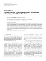
For illustrative purposes Fig. 4 shows the percentage of
improvement of each spread solution when using a very
low fixed threshold. Considering that at the beginning of
the execution the improvements in the local solutions will
be notably larger than at the end, an adaptive procedure
that allows to start with a large threshold and decrease
it with the search progress will improve the efficiency
of the cooperation scheme. The suggested threshold to
begin with is a 10%, that is, incoming solutions that
improve the best known solution in the master process
by at least 10% are spread to the islands as cooperative
solutions. Once the search progresses and most of the

incoming solutions are below this threshold of improvement, the master reduces the threshold to a half. This

procedure is repeated, so that the threshold is reduced,
driven by the incoming solutions (i.e., the search progress
in the islands). Note that if a excessively high threshold is
selected, it will rapidly decrease to an adequate value for
the problem at hand, when the master process ascertains
that there are insufficient incoming solutions below this
threshold.
Second, the master process is used as a scoreboard
intended to dynamically tune the settings of the eSS in
the different islands. As commented above, each island in
the proposed scheme performs a different eSS. An aggressive island performs frequent local searches, trying to
refine the solution very quickly and keeps a small reference set of solutions. It will perform well in problems
with parameter spaces that have a smooth shape. On the
other hand, conservative islands have a large reference set
and perform local searches only sporadically. They spend
more time combining parameter vectors and exploring
the different regions of the parameter space. Thus, they
are more appropriate for problems with rugged parameter spaces. Since the exact nature of the problem at hand
is always unknown, it is recommended to choose, at the
beginning of the scheme, a range of settings that yields
conservative, aggressive, and intermediate islands. However, a procedure that adaptively changes the settings in
the islands during the execution, favoring those settings
that exhibit the highest success, will further improve the
efficiency of the evolutionary search.
There are several configurable settings that determine
the strategy (conservative/aggressive) used by the sequential eSS algorithm, and whose selection may have a great

Percentage of improvement


100

80

60

40

20

0
0

10

20

30

40

50

60

Number of cooperation
Fig. 4 Improvement as a function of cooperation. Percentage of improvement of a new best solution with respect to the previous best known
solution, as a function of the number of cooperation events. Results obtained from benchmark B4, as reported in the Results section



Penas et al. BMC Bioinformatics (2017) 18:52

impact in the algorithm performance. Namely, these settings are:
• Number of elements in the reference set (dimRefSet,
defined in line 1 in Algorithm 1).
• Minimum number of iterations of the eSS algorithm
between two local searches (local.n2, line 11 in
Algorithm 2).
• Balance between intensification and diversification in
the selection of initial points for the local searches
(balance, line 15 in Algorithm 2).
All these settings have qualitatively the same influence
on the algorithm’s behavior: large setting values lead to
conservative executions, while small values lead to aggressive executions.
Designing a self-adaptive procedure that identifies those
islands that are becoming failures and those that are successful is not an easy task. To decide the most promising
islands, the master process serves as a scoreboard where
the islands are ranked according to their potential. In the
rating of the islands, two facts have to be considered: (1)
the number of total communications received in the master from each islands, to identify promising islands among
those that intensively cooperates with new good solutions;
and (2) for each island, the moment when its last solution has been received, to prioritize those islands that
have more recently cooperated. A good balance between
these two factors will produce a more accurate scoreboard. To better illustrate this problem Fig. 5(a) shows,
as an example, a Gantt diagram where the communications are colored in red. Process 1 is the master process,
while process 2-11 are the slaves (islands). At a time of
t = 2000, process 5 has a large number of communications performed, however, all these communications were
performed a considerable time ago. On the other hand,
process 2 has just communicated a new solution, but

presents a smaller number of total communications performed. To accurately update the scoreboard, the rate of
each island is calculated in the master as the product of
the number of communications performed and the time
elapsed from the beginning of the execution until the last
reception from that island. In the example above, process 6 achieves a higher rate because it presents a better
balance between the number of communications and the
time elapsed since the last reception.
Identifying the worst islands is also cumbersome. Those
processes at the bottom of the scoreboard are there
because they do not communicate sufficient solutions or
because a considerable amount of time has passed since
their last communication. However, they can be either
non-cooperating (less promising) islands or more aggressive ones. An aggressive thread often calls the local solver,
performing longer iterations, and thus being unable to

Page 10 of 24

communicate results as often as conservative islands can
do so. To better illustrate this problem, Fig. 5(b) shows a
new Gantt diagram. At a time of t = 60, process 4 will
be at the top of the scoreboard because it often obtains
promising solutions. This is a conservative island. Process 3 will be at the bottom of the scoreboard because
at that time it has not yet communicated a significant
result. The reason is that process 3 is an aggressive slave
that is still performing its first local search. To accurately identify the non-cooperating islands, the master
process would need additional information from islands
that would imply extra messages in each iteration of the
eSS. The solution implemented is that each island decides
by itself whether it is evolving in a promising mode or not.
If an island detects that it is receiving cooperative solutions from the master but it cannot improve its results, it

will send the master a reconfiguration request. The master, will then communicate to this island the settings of the
island on the top of the scoreboard.
Comprehensive overview of the saCeSS algorithm

The pseudocode for the master process is shown in
Algorithm 4, while the basic pseudocode for each slave is
shown in Algorithm 5.
At the beginning of the algorithm, a local variable
present in the master and in each slave is declared to keep
track of the best solution shared in the cooperation step.
The master process sets the initial threshold, initiates the
scoreboard to keep track of the cooperation rate of each
slave, and begins to listen to the requests and cooperations
arriving from the slaves. Each time the master receives
from a slave a solution that significantly improves the current best known solution (BestKnownSol), it increments
the score of this slave on the board.
Each slave creates its own population matrix of ndiverse solutions. Then an initial RefSet is generated for
each process with dimRefSet solutions with the best elements and random elements. Again, different dimRefSet
are possible for different processes. The rest of the operations are performed within each RefSet in each process,
in the same way as in the serial eSS implementation.
Every external iteration of the algorithm, a cooperation
phase is performed to exchange information with the rest
of the processes in the parallel application. Whenever a
process reaches the cooperation phase, it checks if any
message with a new best solution from the master has
arrived at its reception memory buffer. If a new solution
has arrived, the process checks whether this new solution
improves the BestKnownSol or not. If the new solution
improves the current one, the new solution promotes to
be the BestKnownSol. The loop to check the reception of

new solutions must be repeated until there are no more
shared solutions to attend. This is because the execution
time of one external iteration may be very different from


Penas et al. BMC Bioinformatics (2017) 18:52

Page 11 of 24

Fig. 5 Gantt diagrams representing the tasks and cooperation between islands against execution time. Process 1 is the master, and processes 2-11
are slaves (islands). Red dots represent asynchronous communications between master and slaves. Light blue marks represent global search steps,
while green marks represent local search steps. These figures correspond to two different examples, intended to illustrate the design decisions,
described in the text, taken in the self-adaptive procedure to identify successful and failure islands. a Gantt diagram 1 and b Gantt diagram 2

one process to another, due to the diversification strategy explained before. Thus, while a process has completed
only one external iteration, their neighbors may have completed more and several messages from the master may be
waiting in the reception buffer. Then, the BestKnownSol
has to replace the cooperation entry in the process RefSet.

After the reception step, the slave process checks
whether its best solution improves in, at least, an the
BestKnownSol. If this is the case, it updates BestKnownSol
with its best solution and sends it to the master. Note that
the used in the slaves is not the same as the used in
the master process. The slaves use a rather small so that


Penas et al. BMC Bioinformatics (2017) 18:52

Algorithm 4: Self-adaptive Cooperative enhanced

Scatter Search algorithm - saCeSS. Pseudocode for
the master process
1

BestKnownSol = DBL_MAX;

2
3
4

! Initial threshold
=0.1;
nRefuse=0;

5

! Scoreboard information
slaveComm(:)=0;
slaveScore(:)=0;
for i=1 to nslaves do
scoreBoard(i)=i;
end
repeat
! Cooperation step
recvflag=true;
sendflag=false;
while recvflag do
Non_Blocking_Recv(RecvSol,slave,recvflag);
if ((BestKnownSol − RecvSol)/BestKnownSol) <
then

BestKnownSol=RecvSol;
sendflag=true;
! Score slave
slaveComm(slave)++;
slaveScore(slave)=slaveComm(slave)*elapsed
Time();
else
nRefuse++;
end
end
if sendflag then
Non_Blocking_Send(BestKnownSol,slaves);
end

6
7
8
9
10
11
12
13
14
15
16
17
18
19
20
21

22
23
24
25
26
27
28
29
30
31
32
33
34
35
36
37
38
39
40
41
42

! Adapt threshold considering refused solutions
if nRefuse > nslaves then
= /2 ;
nRefuse=0;
end
! Adapt slaves’ settings using scoreboard
recvflag=true;
while recvflag do

Non_Blocking_Recv(Request,slave,recvflag);
Sort(scoreBoard);
Non_Blocking_Send(NewSettings[scoreBoard(0)],
slave);
end
until stopping criterion;

many good solutions will be sent to the master. The master,
in turn, is in charge of selecting those incoming solutions
that are qualified to be spread, thus, its begins with quite
a large value that decreases when the number of refused
solutions increases and no incoming solution overcomes
the current .
Finally, before the end of the iteration, the adaptive
phase is performed. Each slave decides if it is progressing
in the search by checking if:

Page 12 of 24

Algorithm 5: Self-adaptive Cooperative enhanced
Scatter Search algorithm - saCeSS. Pseudocode for
the slave processes
1
2
3
4
5
6
7
8


9
10
11
12
13
14
15
16
17
18
19
20
21
22
23
24
25
26
27
28
29
30
31
32
33
34

35
36

37
38

BestKnownSol = DBL_MAX;
recvSolutions=0;
iter_solver=0;
Neval =0;
Create_Population(ndiverse);
Generate_RefSet(RefSet, dimRefSet);
repeat
! Serial eSS: (1) RefSet order and duplicity check,
(2) Solution combination, (3) RefSet update, (4)
Extra mechanisms and (5) Improvement method
(see Algorithms 1 and 2).
! Cooperation step
sendflag=false;
recvflag=true;
replaceflag=false;
while recvflag do
Non_Blocking_Recv(RecvSol,master,recvflag);
if RecvSol < BestKnownSol then
BestKnownSol=RecvSol;
recvSolutions++;
replaceflag=true;
end
end
if replaceflag then
Replace_Solution(BestKnownSol);
end
if ((BestKnownSol − bestSol)/bestSol) < then

BestKnownSol=bestSol;
sendflag=true;
end
if sendflag then
Non_Blocking_Send(BestKnownSol,master);
Neval =0;
recvSolutions=0;
end
! Adaptive step
if
recvSolutions > (10 × sendSolutions) + 20 && Neval
> (Npar × 5000) then
Non_Blocking_Send(Request,master);
end
Non_Blocking_Recv(NewSettings,master,recvflag);
until stopping criterion;

Neval > Npar × 5000
where Neval is the number of evaluations performed by
this process since its last cooperation with the master
and Npar is the number of parameters of the problem.
Thus, the reconfiguration condition depends on the problem at hand. Besides, if the number of received solutions
is greater than the number of solutions sent, that is, if
other processes are cooperating much more than itself,
the reconfiguration condition is also met. Summarizing,
if a process detects that it is not improving while it is
receiving solutions from the master, it sends a request for
reconfiguration to the master process. The master listens



Penas et al. BMC Bioinformatics (2017) 18:52

to these requests and sends to those slaves the settings of
the most promising ones, i.e., those that are on the top of
the scoreboard.
Finally, the saCeSS algorithm repeats the external loop
until the stopping criterion is met. The current version
can consider three different stopping criteria (or any combination among them): maximum number of evaluations,
maximum execution time and a value-to-reach (VTR).
While the VTR is usually known in benchmark problems
(such as those used below), for a new problem, the VTR
will be, in general, unknown. Thus, in such more realistic
cases, the recommended practice in metaheuristics is to
perform some trial runs and then analyze the convergence
curves in order to find sensible values for the maximum
number of evaluations and/or execution time.
For illustrative purposes, Fig. 6 graphically shows
the self-adaptive Cooperative enhanced Scatter Search
(saCeSS) proposed. Note that different processes (islands)
are executing a different eSS. Since they run asynchronously, they might be in different stages at every
time moment. Thus, cooperation between these different
searches should also be performed in an asynchronous
fashion, avoiding stalls if any of the islands is involved
in a time consuming phase, such as the execution of the
local solver (see process ID 6 in the figure), while other
islands (processes ID 1, ID 3 and ID 5 in the figure) are
in the cooperation phase. When an island cannot attend
to a cooperation reception, the message will be stored in

Page 13 of 24


the process as a pending cooperation, avoiding the blocking of the sender process (see processes ID 3 or ID 5 in
the figure, attending pending cooperations). The master
process (ID 0 in the figure) is in charge of the cooperation between parallel searches and their long-term
behavior. It maintains a scoreboard to guide the adaptive procedure that tunes the settings of the eSS in the
different islands. When an island detects that it is not progressing in its search (see process ID 7 in the figure), it
sends the master a reconfiguration request. The master
communicates, to those islands that request a reconfiguration, the settings of the most promising searches
according to its scoreboard (see process ID 4 in the
figure).

Results and discussion
The proposed self-adaptive cooperative algorithm
(saCeSS) has been applied to a set of benchmarks from
the BioPreDyn-bench suite [66], with the goal of assessing its efficiency in challenging parameter estimation
problems in computational system biology:
• Problem B1 : genome-wide kinetic model of S.
cerevisiae. It contains 276 dynamic states, 44
observed states and 1759 parameters.
• Problem B2 : dynamic model of the central carbon
metabolism of E. coli. It consists of 18 dynamic states,
9 observed states and 116 estimable parameters.

Fig. 6 saCeSS: self-adaptive Cooperative enhanced Scatter Search. An example representation of the different mechanisms of communication and
adaptation proposed in saCeSS


Penas et al. BMC Bioinformatics (2017) 18:52

• Problem B3 : dynamic model of enzymatic and

transcriptional regulation of the central carbon
metabolism of E. coli. It contains 47 dynamic states
(fully observed) and 178 parameters to be estimated.
• Problem B4 : kinetic metabolic model of Chinese
Hamster Ovary (CHO) cells, with 34 dynamic states,
13 observed states and 117 parameters.
• Problem B5 : signal transduction logic model, with 26
dynamic states, 6 observed states and 86 parameters.
• Problem B6 : dynamic model describing the gap gene
regulatory network of the vinegar fly, Drosophila
melanogaster. It consists of three processes
formalized with 108-212 ODEs, and resulting in a
model with 37 unknown parameters.
Different experiments have been conducted using the
saCeSS method, and its performance has been compared
with two different parallel versions of the eSS, namely:
an embarrassingly-parallel non-cooperative enhanced
Scatter Search (np-eSS), and a previous cooperative synchronous version (CeSS) [51]. The np-eSS algorithm consists of np independent eSS runs (being np the number of
available processors) performed in parallel without cooperation between them and reporting the best execution
time of the np runs. Diversity is introduced in these np eSS
runs, alike in the cooperative methods, that is, each one
executes a separate eSS using different strategies.
It should be noted that the eSS [57] and CeSS [51] methods have been originally implemented in Matlab. Both
algorithms have been now coded in F90 to perform an
honest comparison with the proposed saCeSS method.
For the same reason, the CeSS method has been re-written
using the MPI library for the communications between
master and slaves, since its original reported implementation used jPar [67].
The experiments reported here have been performed
in a multicore cluster with 16 nodes powered by two

octa-core Intel Xeon E5-2660 CPUs with 64 GB of RAM.
The cluster nodes were connected through an InfiniBand
FDR network. For problem B3 this cluster could not be
used because the execution of B3 exceeds the maximum
allowed job length. Thus, another multicore heterogeneous cluster was used for this problem that consists of 4
nodes powered by two quadcore Intel Xeon E5420 CPUs
with 16 GB of RAM and 8 nodes powered by two quadcore
Intel Xeon E5520 CPUs with 24 GB of RAM, connected
through a Gigabit Ethernet network.
The computational results shown in this paper were
analyzed from a horizontal view [68], that is, assessing
the performance by measuring the time needed to reach
a given target value. To evaluate the efficiency of the
proposal, experiments with a stopping criteria based on
a value-to-reach (VTR) were performed. The VTR used
was the optimal fitness value reported in [66]. Also, since

Page 14 of 24

comparing different metaheuristic is not an easy task, due
to the substantial dispersion of computational results due
to the stochastic nature of these methods, each experiment reported in this section was performed 20 times and
a statistical study was carried out.
Performance evaluation of the coarse-grained
parallelization and the self-adaptive mechanism

The cooperation between processes in the coarse-grained
parallelization can change the systemic properties of the
eSS algorithm and therefore its macroscopic behavior.
The same happens with the self-adaptive mechanism proposed. Thus, the first set of experiments shown in this

section disables the fine-grained parallelization, since it
does not alter the convergence properties of the algorithm, to evaluate solely the impact of the coarse-grained
parallelization, as well as the self-adaptive mechanism.
Table 1 displays, for each benchmark and each method,
the number of external iterations performed (line 7 in
Algorithm 1), the average number of evaluations needed
to achieve the VTR, the mean and standard deviation
execution time of all the runs in the experiment and
the speedup achieved versus the non-cooperative case
(10-eSS). In these experiments, the computational load
is not shared among processors. Therefore, the total
speedup achieved over the np-eSS method depends on the
impact that the cooperation among processes produces
on achieving a good result, performing less evaluations
and, hence, providing a better performance. We compare the CeSS method, that exchanges the information
based on a time elapsed, and where the information to
be exchanged is the complete RefSet, and the proposed
saCeSS method, that exchanges the information driven
by the quality of the solutions through a star topology
using asynchronous communications and, thus, avoiding
communication delays. Additionally, to better evaluate the
efficiency of the self-adaptive procedure proposed, Table 1
also displays results for two different experiments with the
saCeSS method: experiments where the self-adaptive procedure was disabled, labeled as saCeSS(non-adaptive) in
the table, that is, the settings of the eSS in the different
islands were not dynamically tuned during the execution; and, experiments where this procedure was enabled,
allowing for the adaptive reconfiguration of the islands,
labeled as saCeSS in the table.
The results of the saCeSS (non-adaptive) show that
the cooperation mechanisms and the asynchronous communication protocol proposed in the saCeSS method

improve the results obtained by 10-eSS and CeSS, both
in terms of number of evaluations and execution time.
As regards the CeSS method, the results can be explained
both because the synchronization slows down the processes, since it implies more processes’ stalls while waiting for data, and because of the effectiveness of the


Penas et al. BMC Bioinformatics (2017) 18:52

Page 15 of 24

Table 1 Performance of the coarse-grained parallelization and the self-adaptive scheme proposed
P

B1

B2

B3

B4

B5

B6

Method

Mean iter±std

Mean evals±std


Mean time±std(s)

Speedup

10-eSS

80±30

199214±44836

5378 ± 1070

-

CeSS (τ = 700s)

109±49

188131±82834

6487 ± 3226

0.83

CeSS (τ = 1400s)

122±41

175331±98255


5018 ± 1477

1.07

saCeSS( non-adaptive)

92±35

143145±61828

3759 ± 976

1.43

saCeSS

62±21

92122±35058

2753 ± 955

1.95

10-eSS

450±167

1504503±541257


1914 ± 714

-

CeSS ( τ = 400s)

452±278

1637125±1016688

2459 ± 2705

0.78

CeSS ( τ = 800s)

508±205

1802917±690613

1911 ± 1103

1.00

saCeSS( non-adaptive)

440±192

1528793±647677


1918 ± 833

1.00

saCeSS

846±982

1247699±1222378

1694 ± 1677

1.13

10-eSS

10062±2528

66915128±15623835

511166 ± 135988

-

CeSS(τ = 50000s)

7288±5551

52592578±35513874


332721 ± 245829

1.53

saCeSS( non-adaptive)

4323±3251

32604331±23357322

251305 ± 209082

2.03

saCeSS

4113±3130

27647470±21488783

229888 ± 238970

2.22

10-eSS

99±121

2230089±2068300


750 ± 692

-

CeSS (τ = 100s)

140±386

1665954±2921838

817 ± 1909

0.92

CeSS (τ = 200s)

119±87

1649723±1024833

518 ± 428

1.45

saCeSS( non-adaptive)

39±30

1163458±927751


402 ± 303

1.86

saCeSS

35±24

1017956±728328

343 ± 240

2.18

10-eSS

16±4

69448±14570

901 ± 197

-

CeSS (τ = 200s)

11±4

108481±36190


1481 ± 634

0.61

CeSS (τ = 400s)

14±3

94963±20172

996 ± 264

0.90

saCeSS( non-adaptive)

10±2

49622±9530

637 ± 131

1.42

saCeSS

10±3

51076±12696


658 ± 174

1.37

10-eSS

4659±3742

9783720±8755231

8217 ± 7536

-

CeSS ( τ = 1000s)

5919±5079

10475485±8978383

8109 ± 7441

1.01

CeSS ( τ = 2000s)

6108±6850

10778260±12157617


7878 ± 9400

1.04

saCeSS( non-adaptive)

2501±1517

4394243±2689489

3638 ± 2302

2.26

saCeSS

1500±1265

2594741±2214235

2177 ± 1933

3.77

Execution time and speedup results using 10 processors. Stopping criteria: VTRB1 = 1.3753 × 104 , VTRB2 = 2.50 × 102 , VTRB3 = 3.7 × 10−1 , VTRB4 = 55, VTRB5 = 4.2 × 103 ,
VTRB6 = 1.0833 × 105

information exchanged. The results of the saCeSS show
that the self-adaptive approach improves the previous

results even more. The main goal of this approach
is to reduce the impact that the initial choice of the
configurable settings may have in the evolution of the
method. For instance, one issue of the CeSS algorithm
is the selection of the migration time (τ ), that is, the
time between information sharing. On the one hand,
this time has to be long enough to allow each of the
threads to exploit the eSS capabilities. On the other hand,
if the time is too long, cooperation will happen only

sporadically, reducing its efficiency. On the contrary, in
the saCeSS method proposed, the initial selection of the
threshold to spread a cooperative solution, as well as
the selection of the other configurable settings of the
eSS method, will change adaptively during the execution
progress.
When dealing with stochastic optimization solvers, it
is important to evaluate the dispersion of the computational results. Figure 7 illustrates how the proposed
saCeSS reduces the variability of execution time in the
non-cooperative 10-eSS method. This is an important


Penas et al. BMC Bioinformatics (2017) 18:52

Page 16 of 24

Fig. 7 Hybrid violin/Box plots of the execution times using 10 processes. Results for experiments reported in Table 1.The green asterisks correspond
to the mean and light blue boxes illustrate the distribution of the results. Each box with a strong blue contour represents a typical boxplot: the
central red line is the median, the edges of the box are the 25th and 75th percentiles, and outliers are plotted with red crosses. (a) B1, (b) B2, (c) B3,
(d) B4, (e) B5 and (f) B6


feature of the saCeSS, because it reduces the average
execution time for each benchmark. For instance, even
in the B2 problem, where the mean execution time is

similar in the non-cooperative and the cooperative executions, the dispersion of the results is reduced in the
cooperative case.


Penas et al. BMC Bioinformatics (2017) 18:52

Page 17 of 24

Finally, to prove the significance of the results, a nonparametric statistical analysis has been applied to the
final runtimes of the experiments over each test problem.
Recent studies show that the most appropriate methods to
compare the performance of different metaheuristics are
the nonparametric procedures [69]. In this work we have
applied the Kruskal-Wallis test [70] followed by Dunn’s
test [71], that reports the results among multiple pairwise
comparisons after the Kruskall-Wallis test. The objective is to explain if the observed differences among final
runtimes for each problem are due to the optimization
method used (i.e., np-eSS, CeSS and saCeSS) or to pure
randomness. Table 2 shows, for each problem, the pvalues of Dunn’s test for every pair comparison after the
Kruskall-Wallis test application. Table 3 shows, for each
problem, the classification of methods in groups at 95%
confidence level according to the p-values shown above.
As shown in Tables 2 and 3, the statistical results reveal
that saCeSS shows better performance than the other two
methods in the problems considered. It is clear for problems B1, B3, B5 and B6. For problems B2 and especially B4,

the differences are not as significant as in the other problems. For B2, the reason is the outlier in one of the runs
with saCeSS in problem B2, which damages the results
since it is the worst value among all runs and methods for
this problem. For B4, the reason is the high dispersion of
the results, together with the fact that many experiments
achieved the convergence in the first iterations of the algorithm (note the swelling at the bottom of the violin/box
plots in Fig. 7), before the cooperation turned into effective, or the self-adaptive procedure became operational,
thus, reducing the difference among the three algorithms.
The CeSS method presents an important issue related
to its scalability, since the cooperation among islands is
carried through a synchronous communication step. To
assess the scalability of the coarse-grained parallelization proposed in saCeSS, experiments were carried out
using 1 (that is a single eSS), 10, 20 and 40 processors. The convergence curves for B2 benchmark (see
Additional file 1 for the others problems) are shown in
Fig. 8. This curves represent the logarithm of the objective function value against the execution time for those
experiments that fall in the median values of the results
distribution. Similar results are obtained for the rest of the
benchmarks, and they are reported in the supplementary

Table 2 p-values of the pairwise comparisons provided by the
Dunn’s test
B1

B2

B3

B4

B5


B6

saCeSS vs CeSS

0.0000

0.0630

0.0380

0.1924

0.0000

0.0000

saCeSS vs 10-eSS

0.0000

0.0115

0.0000

0.0324

0.0001

0.0000


CeSS vs 10-eSS

0.1850

0.2289

0.0006

0.1641

0.2128

0.3964

Table 3 Group classification of the optimization methods at 95%
confidence level
B2a

B1
saCeSS

A

B3

A

CeSS


B

10-eSS

B

A

B4

A
B
B

B5

A
B

A
C

B6

A

A

B


B

B

B

B

B

a For problem B2, the classification at 90% confidence interval is:

saCeSS(A), CeSS(B), np-eSS(B)

information. As it can be observed, when the number of
processors grows, the saCeSS method keeps on improving the convergence results. This is due to the proposed
asynchronous communication protocol. However, as the
number of cooperative processes increases, the improvement in the algorithm performance is restrained. This is
readily justified, because the self-adaptive mechanism will
drive the different processes from different initial parameters to those settings that obtain successful results, which,
in the long term, means that having a larger number of
processes does not aim to a larger diversity and better
results. Thus, the hybrid MPI+OpenMP proposal aims
to improve the performance results when the number
of processors increases, by combining the MPI stimulation on diversification in the search with the OpenMP
intensification.
Performance evaluation of the hybrid MPI+OpenMP
proposal

The goal of the fine-grained parallelization proposed in

this paper is to perform the evaluation of the obtained
solutions in parallel threads, thus, accelerating the execution without altering the properties of the algorithm. As
already commented in previous sections, the scalability of
the fine-grained parallelization is limited in the eSS algorithm, due to the small dimRefSet. Also, the workload is
uneven, since different evaluations lead some threads to
be busy for longer times. Thus, the dynamic schedule used
allows the threads with small workloads to go after other
chunks of work, and hopefully, balance the work between
threads. But it introduces a large overhead at runtime, as
work has to be taken off of a queue.
Table 4 shows the performance and scalability of the
hybrid MPI+OpenMP implementation proposed in this
work. Benchmarks B3 and B6 were excluded of these
evaluations: B3 due to our lack of available resources
to run such long executions, and B6 since its currently
available implementation could not be parallelized using
the OpenMP library. Note that the np-eSS algorithm
was executed also using 10, 20 and 40 processes (noncooperative), to perform a fair comparison with saCeSS
using 10, 20 and 40 processors respectively. The speedup
was calculated accordingly. In most of the cases, the
hybrid configurations obtain better performance than


Penas et al. BMC Bioinformatics (2017) 18:52

Page 18 of 24

2000
eSS (1 proc)
saCeSS (10 proc_MPI)

saCeSS (20 proc_MPI)
saCeSS (40 proc_MPI)

f(x)

1000

250
50

100

1000

5000

10000

Wall-time (s)

Fig. 8 Scalability of self-adaptive Cooperative enhanced Scatter Search (saCeSS) using 1, 10, 20 and 40 processors in problem B2. Note that the
saCeSS method using 1 MPI process is equivalent to the eSS method using 1 processor. For each method, the convergence curves that are closer to
the median of the results distribution are shown in the figure. Detailed distributions for all the benchmarks can be found in Additional file 1

other configurations that only use MPI processes. In general, results show that, for the same number of processors,
those hybrid configurations that achieve a good balance
between intensification and diversification perform more
effectively. For instance, the configuration of 5 MPI processes with 4 OpenMP threads each, achieves, in general,
better speedup than the configuration with 10 MPI processes with 2 OpenMP threads each, while both use 20
processors. The exception is benchmark B4, whose performance is heavily affected by the number of different

processes cooperating. That is, benchmark B4 greatly benefits from the diversity introduced with the scalability in
the number of MPI processes versus the intensification
of the OpenMP search. Thus, for benchmark B4, configurations using all the available processors to run MPI
cooperative processes perform better.
Figure 9 shows, for B2 benchmark (see Additional file 1
for the others problems), the convergence curves for those
experiments that fall in the median values of the results
distribution. Similar results are obtained for the rest of
the benchmarks, and they are reported in the supplementary information. The performance of 40 individual, non
cooperative processes, is compared to the performance of
saCeSS method with different hybrid configurations using
40 processors in all of them. As it has already been pointed
out, when the number of available processors increases,
hybrid MPI+OpenMP configurations will improve the

performance versus a solely coarse-grained parallelization
(see Fig. 9). This is an important result because it allows
us to predict a good performance of this method on HPC
systems, built as clusters of multicore nodes, where MPI
processes would be located in different nodes, improving diversification, while, within each node, the OpenMP
threads would intensify the search.
Finally, Fig. 10 compares the results obtained by the
proposed saCeSS method and the results reported in
the BioPreDyn-bench suite [66]. Note that, although
these figures correspond to a partially different language
implementation of eSS (Matlab and C, as reported in
[66]), the cost functions and the associated dynamics were
computed using the same C code in both cases. It can
be observed that the parallel cooperative scheme significantly reduces the execution time in the very complex
problems as B1 (1 week vs 1 hour) or B3 problem (10

days vs less than 46 hours). These figures can be especially illustrative for those interested in the potential of
HPC in general, and the saCeSS method in particular, in
the solution of parameter estimation problems.
Comparison with other parallel metaheuristics

In order to properly evaluate the novel parallel method
presented here, we now compare it with a parallel version of another state of the art metaheuristic, Differential
Evolution (DE [72]). Previous works in the literature have


Penas et al. BMC Bioinformatics (2017) 18:52

Page 19 of 24

Table 4 Performance of the hybrid MPI+OpenMP saCeSS and scalability analysis when the number of processors grows
P

Method

# proc. config.

Mean iter±std

Mean evals±std

Mean time±std(s)

Speedup

# (MPI x OpenMP)

B1

B2

B4

10-eSS

10

80±30

199214±44836

5378 ± 1070

-

saCeSS

10 (10 x 1)

62±21

92122±35058

2753 ± 955

1.95


saCeSS

10 (5 x 2)

76±40

88186±46200

2762 ± 1273

1.95

20-eSS

20

106±34

304972±88870

4524 ± 942

-

saCeSS

20 (20 x 1)

79±38


218871±107769

3125 ± 1349

1.45

saCeSS

20 (10 x 2)

86±43

147268±75752

2299 ± 1199

1.97

saCeSS

20 (5 x 4)

54±19

68907±27132

1288 ± 380

3.51


40-eSS

40

79±21

455091±121875

3662 ± 718

-

saCeSS

40 (40 x 1)

51±19

274628±115644

2070 ± 650

1.77

saCeSS

40 (20 x 2)

64±27


205766±93753

1743 ± 759

2.10

saCeSS

40 (10 x 4)

58±30

111804±61212

1130 ± 535

3.24

saCeSS

40 (5 x 8)

57±29

82414±38357

1078 ± 494

3.39


10-eSS

10

450±167

1504503±541257

1914 ± 714

-

saCeSS

10 (10 x 1)

846±982

1247699±1222378

1694 ± 1677

1.13

saCeSS

10 (5 x 2)

630±275


916166±357665

1298 ± 700

1.47

20-eSS

20

355±130

2306298±851619

1465 ± 546

-

saCeSS

20 (20 x 1)

649±287

1901601±747379

1345 ± 619

1.09


saCeSS

20 (10 x 2)

904±646

1388211±854461

962 ± 616

1.52

saCeSS

20 (5 x 4)

609±244

925076±353594

734 ± 320

2.00

40-eSS

40

297±108


3878818±1478105

1223 ± 447

-

saCeSS

40 (40 x 1)

571±542

3286363±2593258

1326 ± 1764

0.92

saCeSS

40 (20 x 2)

766±863

2185567±2228163

951 ± 1468

1.29


saCeSS

40 (10 x 4)

756±243

1309744±446419

506 ± 180

2.42

saCeSS

40 (5 x 8)

522±290

801661±380553

353 ± 162

3.46

10-eSS

10

99±121


2230089±2068300

750 ± 692

-

saCeSS

10 (10 x 1)

35±24

1017956±728328

343 ± 240

2.18

saCeSS

10 (5 x 2)

177±269

1854102±2331070

916 ± 1210

0.82


20-eSS

20

18±22

1206948±1177645

176 ± 203

-

saCeSS

20 (20 x 1)

11±8

819845±548341

111 ± 93

1.58

saCeSS

20 (10 x 2)

30±23


898459±657350

215 ± 169

0.82

saCeSS

20 (5 x 4)

294±692

2090044±3980316

736 ± 1453

0.24

40-eSS

40

12±13

1811454±1608998

121 ± 141

-


saCeSS

40 (40 x 1)

9±5

1254545±603925

78 ± 51

1.55

saCeSS

40 (20 x 2)

26±26

1523817±1267964

159 ± 160

0.76

saCeSS

40 (10 x 4)

37±50


878008±1178953

168 ± 238

0.72

saCeSS

40 (5 x 8)

159±692

1666511±3980316

490 ± 446

0.25


Penas et al. BMC Bioinformatics (2017) 18:52

Page 20 of 24

Table 4 Performance of the hybrid MPI+OpenMP saCeSS and scalability analysis when the number of processors grows (Continued)
B5

10-eSS

10


16±4

69448±14570

901 ± 197

-

saCeSS

10 (10 x 1)

10±3

51076±12696

658 ± 174

1.37

saCeSS

10 (5 x 2)

11±3

36090±8761

520 ± 136


1.73

20-eSS

20

11±2

106051±17602

685 ± 127

-

saCeSS

20 (20 x 1)

10±2

99995±21070

654 ± 151

1.05

saCeSS

20 (10 x 2)


9±2

52419±12040

368 ± 92

1.86

saCeSS

20 (5 x 4)

10±3

38427±10523

331 ± 97

2.07

40-eSS

40

10±2

192192±29082

618 ± 102


-

saCeSS

40 (40 x 1)

8±2

161687±40392

514 ± 138

1.20

saCeSS

40 (20 x 2)

9±2

100315±17758

350 ± 68

1.76

saCeSS

40 (10 x 4)


11±2

64594±13173

280 ± 61

2.21

saCeSS

40 (5 x 8)

11±3

45854±11607

248 ± 67

2.48

Execution time and speedup results. Stopping criteria: VTRB1 = 1.3753 × 104 , VTRB2 = 2.50 × 102 , VTRB3 = 3.7 × 10−1 , VTRB4 = 55, VTRB5 = 4.2 × 103 , VTRB6 = 1.0833 × 105

already pointed out that, for sequential implementations,
eSS performs better than DE in those problems where
local searches are instrumental in refining the solution
[51]. Thus, to ensure a more fair comparison here, we
chose a parallel DE implementation (asynPDE [43]) that

performs a global search through an asynchronous parallel implementation based on a cooperative island-model,
and that also improves the local search phase by means of

several heuristics also used in the eSS (i.e. an efficient local
solver, a tabu list and a logarithmic space search).

Fig. 9 Comparative between non-cooperative enhanced Scatter Search (eSS) and self-adaptive Cooperative enhanced Scatter Search (saCeSS)
using 40 processors in problem B2. The performance of 40 individual, non-cooperative eSS is compared with different hybrid configurations of the
saCeSS method using 40 processors. For each method, the convergence curves that are closer to the median of the results distribution are shown in
the figure. Detailed distributions for all the benchmarks can be found in Additional file 1


Penas et al. BMC Bioinformatics (2017) 18:52

Page 21 of 24

Fig. 10 Performance acceleration of saCeSS versus eSS (as reported in [66]). Bars show wall-clock times for each solver and benchmark problem,
with the numbers over saCeSS bars indicating the overall acceleration obtained. Computations with saCeSS were carried out with 10 processors
while computations with eSS were carried out with 1 processor

2000
saCeSS (10 proc_MPI)
saCeSS (5 proc_MPI x 2 th_openMP)
asynPDE (10 proc_MPI)

f(x)

1000

250
20

100


1000

5000

Wall-time (s)
Fig. 11 Comparison of the convergence curves of asynchronous parallel Differential Evolution (asynPDE) and self-adaptive Cooperative enhanced
Scatter Search (saCeSS) using 10 processors in problem B2. For each method, the convergence curves that are closer to the median of the results
distribution are shown in the figure. Detailed distributions for all the benchmarks can be found in Additional file 1


Penas et al. BMC Bioinformatics (2017) 18:52

Page 22 of 24

The convergence curves, considering problem B2 (see
Additional file 1 for the others problems), of the asynPDE and the saCeSS algorithms for 10 and 20 processors
are shown in Figs. 11 and 12 respectively. These figures
represent the convergence curves for those experiments
that fall in the median values of the results distribution.
Although the best configuration for the saCeSS method is
a hybrid MPI+OpenMP one, since the asynPDE method
only performs a coarse-grained parallelization, for comparison purposes the convergence curves of saCeSS using
only MPI processes are shown. As can be seen, in all
cases asynPDE is significantly outperformed by saCeSS.
Results for the other benchmarks can be found in the
supplementary information.

Conclusions
In this contribution we present a novel parallel method for

global optimization in computational systems biology: a
self-adaptive parallel cooperative enhanced scatter search
algorithm (saCeSS). A hybrid MPI+OpenMP implementation is proposed combining a coarse-grained parallelization, focused on stimulating the diversification in the
search and the cooperation between different processes,

with a fine-grained parallelization, aimed at accelerating the computation by performing separate evaluations
in parallel. This novel approach results in a much more
effective way of cooperation between different processes
running different configurations of the scatter search algorithm.
The new proposed approach has four main features: (i) a
coarse-grained parallelization using a centralized masterslave approach, where the master is in charge of the control of the communications between slaves (islands) and
serves as a scoreboard to dynamically tune the settings of
the islands based on its individual progress; (ii) a cooperation between processes driven by the quality of the
solution obtained during the execution progress, instead
of by time elapsed; (iii) an asynchronous communication
protocol that minimizes processes’ halts, thus improving
the efficiency in a computational unbalanced scenario;
and (iv) a fine-grained parallelization is included in each
process to perform separate cost-function evaluations in
parallel and, thus, accelerate the global search.
The proposed saCeSS method was evaluated considering a suite of very challenging benchmark problems
from the domain of computational systems biology. The

2000
saCeSS (20 proc_MPI)
saCeSS (5 proc_MPI x 4 th_openMP)
asynPDE (20 proc_MPI)

f(x)


1000

250
20

100

1000

5000

Wall-time (s)
Fig. 12 Comparison of the convergence curves of asynchronous parallel Differential Evolution (asynPDE) and self-adaptive Cooperative enhanced
Scatter Search (saCeSS) using 20 processors in problem B2. For each method, the convergence curves that are closer to the median of the results
distribution are shown in the figure. Detailed distributions for all the benchmarks can be found in Additional file 1


Penas et al. BMC Bioinformatics (2017) 18:52

computational results show that saCeSS attains a very
significant reduction in the convergence time through
cooperation of the parallel islands (from days to minutes in several cases, using a small number of processors). A nonparametric statistical analysis shows that the
saCeSS method significantly outperforms other parallel
eSS approaches, such as an embarrassingly-parallel noncooperative eSS algorithm, and a previous synchronous
cooperative proposal.
These results indicate that parameter estimation in
large-scale dynamic models of biological systems can
be feasible even when using small and low-cost parallel machines, thus opening new perspectives towards the
development and calibration of whole-cell models [73].


Additional file
Additional file 1: Supplementary info document. This document is a
complete report for all experiments performed for this work. (PDF 9 305 kb)
Abbreviations
SS: Scatter search; eSS: enhanced scatter search; CeSS: Cooperative enhanced
scatter search; saCeSS: Self-Adaptive cooperative enhanced scatter search;
MPI: Message passing interface; openMP: Open multi-processing; NLP:
NonLinear programming; DAE: Differential algebraic equations; HPC: High
performance computing; F90: Fortran 90; DE: Differential evolution; asynPDE:
asynchronous parallel differential evolution; VTR: Value to reach
Acknowledgements
The authors acknowledge financial support from the Spanish Ministerio de
Economía y Competitividad and from the Galician Government. They
acknowledge support of the publication fee by the CSIC Open Access
Publication Support Initiative through its Unit of Information Resources for
Research (URICI). DRP acknowledges financial support from the MICINN-FPI
programme.
Funding
This research received financial support from the Spanish Ministerio de
Economía y Competitividad (and the FEDER) through the “MultiScales” project
(subprojects DPI2011-28112-C04-03, DPI2011-28112-C04-04),
“SYNBIOFACTORY” (DPI2014-55276-C5-2-R), TIN2013-42148-P and TIN201675845-P, and from the Galician Government under the Consolidation Program
of Competitive Research Units (Networks ref. R2014/041 and ref. R2016/045,
and competitive reference groups GRC2013/055). DRP acknowledges financial
support from the MICINN-FPI programme. We acknowledge support of the
publication fee by the CSIC Open Access Publication Support Initiative
through its Unit of Information Resources for Research (URICI).
Availability of data and materials
The datasets supporting the conclusions of this article are included within the
article and its additional files. The souce code of saCeSS is available at https://

bitbucket.org/DavidPenas/sacess-library/.
Authors’ contributions
JRB, PG and RD conceived the study. PG, JRB and RD coordinated the study.
DRP and PG implemented the methods with help from JAE and carried out all
the computations. DRP, PG, JAE and JRB analyzed the results. PG and DRP
drafted the initial manuscript. All authors contributed to writing the final
manuscript, reading and approving the submitted version.
Competing interests
The authors declare that they have no competing interests.
Consent for publication
Not applicable.

Page 23 of 24

Ethics approval and consent to participate
Not applicable.
Author details
1 BioProcess Engineering Group, IIM-CSIC, Eduardo Cabello 6, 36208 Vigo,

Spain. 2 Computer Architecture Group, Universidade da Coruña, Campus de
Elviña s/n, 15071 A Coruña, Spain. 3 Department of Applied Mathematics and
Statistics, Universidad Politécnica de Cartagena, c/ Dr. Fleming s/n, 30202
Cartagena, Spain.
Received: 24 February 2016 Accepted: 24 December 2016

References
1. Gadkar KG, Gunawan R, Doyle FJ. Iterative approach to model
identification of biological networks. BMC bioinformatics. 2005;6(1):1.
2. Doyle FJ, Stelling J. Systems interface biology. J Royal Soc Interface.
2006;3(10):603–16.

3. Kremling A, Saez-Rodriguez J. Systems biology–an engineering
perspective. J biotechnol. 2007;129(2):329–51.
4. Hasenauer J, Waldherr S, Wagner K, Allgower F. Parameter identification,
experimental design and model falsification for biological network
models using semidefinite programming. Syst Biol IET. 2010;4(2):119–30.
5. Jaeger J, Monk NA. Reverse engineering of gene regulatory networks.
Learn infer comput syst biol. 20109–34.
6. Kiparissides A, Koutinas M, Kontoravdi C, Mantalaris A, Pistikopoulos EN.
’closing the loop’ in biological systems modeling - from the in silico to the
in vitro. Automatica. 2011;47(6):1147–1155.
7. Menolascina F, Siciliano V, Di Bernardo D. Engineering and control of
biological systems: a new way to tackle complex diseases. FEBS letters.
2012;586(15):2122–128.
8. Villaverde AF, Banga JR. Reverse engineering and identification in
systems biology: strategies, perspectives and challenges. J Royal Soc
Interface. 2014;11(91):20130505.
9. Sunnåker M, Stelling J. Model Extension and Model Selection In: Geris L,
Gomez-Cabrero D, editors. Uncertainty in Biology: A Computational
Modeling Approach. Cham: Springer; 2016. p. 213–41.
10. Kaltenbach HM, Dimopoulos S, Stelling J. Systems analysis of cellular
networks under uncertainty. FEBS letters. 2009;583(24):3923–930.
11. Schaber J, Liebermeister W, Klipp E. Nested uncertainties in biochemical
models. Systems Biology, IET. 2009;3(1):1–9.
12. Vanlier J, Tiemann C, Hilbers P, van Riel N. Parameter uncertainty in
biochemical models described by ordinary differential equations. Math
Biosci. 2013;246(2):305–14.
13. Kirk P, Babtie A, Stumpf M. Systems biology (un) certainties. Science.
2015;350(6259):386–8.
14. Kirk P, Silk D, Stumpf MPH. Reverse Engineering Under Uncertainty In:
Geris L, Gomez-Cabrero D, editors. Uncertainty in Biology: A

Computational Modeling Approach. Cham: Springer; 2016. p. 15–32.
15. Ballarini P, Guido R, Mazza T, Prandi D. Taming the complexity of
biological pathways through parallel computing. Brief Bioinform.
2009;10(3):278–88.
16. Dematté L, Prandi D. GPU computing for systems biology. Brief
Bioinform. 2010;11(3):323–33.
17. Zhou Y, Liepe J, Sheng X, Stumpf MP, Barnes C. GPU accelerated
biochemical network simulation. Bioinformatics. 2011;27(6):874–6.
18. Kent E, Hoops S, Mendes P. Condor-copasi: high-throughput computing
for biochemical networks. BMC systems biology. 2012;6(1):91.
19. Smallbone K, Mendes P. Large-scale metabolic models: From
reconstruction to differential equations. Ind Biotechnol. 2013;9(4):179–84.
20. Stanford NJ, Lubitz T, Smallbone K, Klipp E, Mendes P, Liebermeister W.
Systematic construction of kinetic models from genome-scale metabolic
networks. PloS ONE. 2013;8(11):79195.
21. Almquist J, Cvijovic M, Hatzimanikatis V, Nielsen J, Jirstrand M. Kinetic
models in industrial biotechnology - Improving cell factory performance.
Metab Eng. 2014;24:1–22.
22. Link H, Christodoulou D, Sauer U. Advancing metabolic models with
kinetic information. Curr Opin Biotechnol. 2014;29:8–14.
23. Miskovic L, Tokic M, Fengos G, Hatzimanikatis V. Rites of passage:
requirements and standards for building kinetic models of metabolic
phenotypes. Curr Opin Biotechnol. 2015;36:146–53.


Penas et al. BMC Bioinformatics (2017) 18:52

24. Cvijovic M, Almquist J, Hagmar J, Hohmann S, Kaltenbach HM, Klipp E,
Krantz M, Mendes P, Nelander S, Nielsen J, et al. Bridging the gaps in
systems biology. Mol Gen Genomics. 2014;289(5):727–34.

25. Le Novère N. Quantitative and logic modelling of molecular and gene
networks. Nat Rev Genet. 2015;16(3):146–58.
26. Karr JR, Sanghvi JC, Macklin DN, Gutschow MV, Jacobs JM, Bolival B,
Assad-Garcia N, Glass JI, Covert MW. A whole-cell computational model
predicts phenotype from genotype. Cell. 2012;150(2):389–401.
27. Macklin DN, Ruggero NA, Covert MW. The future of whole-cell modeling.
Curr Opin Biotechnol. 2014;28:111–5.
28. Liu Y, Gunawan R. Parameter estimation of dynamic biological network
models using integrated fluxes. BMC Syst Biol. 2014;8(1):1.
29. Meyer P, Cokelaer T, Chandran D, Kim KH, Loh PR, Tucker G, Lipson M,
Berger B, Kreutz C, Raue A, et al. Network topology and parameter
estimation: from experimental design methods to gene regulatory
network kinetics using a community based approach. BMC Syst Biol.
2014;8(1):13.
30. Cedersund G, Samuelsson O, Ball G, Tegnér J, Gomez-Cabrero D.
Optimization in Biology Parameter Estimation and the Associated
Optimization Problem In: Geris L, Gomez-Cabrero D, editors. Uncertainty
in Biology: A Computational Modeling Approach. Cham: Springer; 2016.
p. 177–97.
31. Mendes P, Kell D. Non-linear optimization of biochemical pathways:
applications to metabolic engineering and parameter estimation.
Bioinformatics. 1998;14(10):869–83.
32. Banga J, Balsa-Canto E. Parameter estimation and optimal experimental
design. Essays Biochem. 2008;45:195–210.
33. Ashyraliyev M, Fomekong-Nanfack Y, Kaandorp JA, Blom JG. Systems
biology: parameter estimation for biochemical models. Febs J.
2009;276(4):886–902.
34. Sun J, Garibaldi JM, Hodgman C. Parameter estimation using
metaheuristics in systems biology: a comprehensive review. Comput Biol
Bioinforma IEEE/ACM Trans. 2012;9(1):185–202.

35. Gábor A, Banga JR. Robust and efficient parameter estimation in dynamic
models of biological systems. BMC Syst Biol. 2015;9(1):74.
36. Perkins TJ, Jaeger J, Reinitz J, Glass L. Reverse engineering the gap gene
network of drosophila melanogaster. PLOS Comput Biol. 2006;2(5):51.
37. Ji X, Xu Y. libsres: a c library for stochastic ranking evolution strategy for
parameter estimation. Bioinformatics. 2006;22(1):124–6.
38. Jostins L, Jaeger J. Reverse engineering a gene network using an
asynchronous parallel evolution strategy. BMC Syst Biol. 2010;4(1):17.
39. Zi Z. Sbml-pet-mpi: a parallel parameter estimation tool for systems
biology markup language based models. Bioinformatics. 2011;27(7):
1028–1029.
40. Fomekong-Nanfack Y, Kaandorp JA, Blom J. Efficient parameter
estimation for spatio-temporal models of pattern formation: case study of
drosophila melanogaster. Bioinformatics. 2007;23(24):3356–363.
41. Adams R, Clark A, Yamaguchi A, Hanlon N, Tsorman N, Ali S, Lebedeva
G, Goltsov A, Sorokin A, Akman OE, et al. Sbsi: an extensible distributed
software infrastructure for parameter estimation in systems biology.
Bioinformatics. 2013;29(5):664–5.
42. Lee WP, Hsiao YT, Hwang WC. Designing a parallel evolutionary
algorithm for inferring gene networks on the cloud computing
environment. BMC Syst Biol. 2014;8(1):5.
43. Penas D, Banga J, González P, Doallo R. Enhanced parallel differential
evolution algorithm for problems in computational systems biology. Appl
Soft Comput. 2015;33:86–99.
44. Rodriguez-Fernandez M, Egea JA, Banga JR. Novel metaheuristic for
parameter estimation in nonlinear dynamic biological systems. BMC
bioinforma. 2006;7(1):483.
45. Egea JA, Martí R, Banga JR. An evolutionary method for complex-process
optimization. Comput Oper Res. 2010;37(2):315–24.
46. Jia G, Stephanopoulos G, Gunawan R. Incremental parameter estimation

of kinetic metabolic network models. BMC Syst. Biol. 2012;6(1):1.
47. Becker K, Balsa-Canto E, Cicin-Sain D, Hoermann A, Janssens H, Banga
JR, Jaeger J. Reverse-engineering post-transcriptional regulation of gap
genes in drosophila melanogaster. PLoS Comput Biol. 2013;9(10):1003281.
48. de Hijas-Liste GM, Klipp E, Balsa-Canto E, Banga JR. Global dynamic
optimization approach to predict activation ins metabolic pathways. BMC
Syst Biol. 2014;8(1):1.
49. Henriques D, Rocha M, Saez-Rodriguez J, Banga JR. Reverse engineering
of logic-based differential equation models using a mixed-integer
dynamic optimization approach. Bioinformatics. 2015;31(18):2999–3007.

Page 24 of 24

50. Fan M, Kuwahara H, Wang X, Wang S, Gao X. Parameter estimation
methods for gene circuit modeling from time-series mrna data: a
comparative study. Brief Bioinform. 2015;16(6):987–99.
51. Villaverde AF, Egea JA, Banga JR. A cooperative strategy for parameter
estimation in large scale systems biology models. BMC Syst Biol.
2012;6(1):75.
52. Esposito WR, Floudas CA. Global optimization for the parameter
estimation of differential-algebraic systems. Ind Eng Chem Res.
2000;39(5):1291–1310.
53. Moles CG, Mendes P, Banga JR. Parameter estimation in biochemical
pathways: a comparison of global optimization methods. Genome Res.
2003;13(11):2467–474.
54. Polisetty PK, Voit EO, Gatzke EP. Identification of metabolic system
parameters using global optimization methods. Theor Biol Med Model.
2006;3(1):4.
55. Glover F, Laguna M, Martí R. Fundamentals of scatter search and path
relinking. Control Cybern. 2000;29(3):652–84.

56. Glover F. A template for scatter search and path relinking. In: Selected
Papers from the Third European Conference on Artificial Evolution. AE ’97.
London: Springer; 1998. p. 3–54.
57. Egea JA, Balsa-Canto E, García M-SG, Banga JR. Dynamic optimization of
nonlinear processes with an enhanced scatter search method. Ind Eng
Chem Res. 2009;48(9):4388–401.
58. Beyer HG, Schwefel HP. Evolution strategies – a comprehensive
introduction. Nat Comput. 2002;1(1):3–52.
59. Crainic TG, Toulouse M. Parallel Strategies for Meta-heuristics. Montréal,
Québec: Springer; 2003.
60. Alba E. Parallel Metaheuristics: A New Class of Algorithms. NJ:
Wiley-Interscience; 2005.
61. Alba E, Luque G, Nesmachnow S. Parallel metaheuristics: recent
advances and new trends. Int Trans Oper Res. 2013;20(1):1–48.
62. Jin H, Jespersen D, Mehrotra P, Biswas R, Huang L, Chapman B. High
performance computing using mpi and openmp on multi-core parallel
systems. Parallel Comput. 2011;37(9):562–75.
63. Toulouse M, Crainic T, Gendreau M. Communication issues in designing
cooperative multi-thread parallel searches In: Osman I, Kelly J, editors.
Meta-Heuristics. Montréal, Québec: Springer; 1996. p. 503–22.
64. Toulouse M, Crainic TG, Thulasiraman K. Global optimization properties
of parallel cooperative search algorithms: a simulation study. Parallel
Comput. 2000;26(1):91–112.
65. Toulouse M, Crainic TG, Sansó B. Systemic behavior of cooperative
search algorithms. Parallel Comput. 2004;30(1):57–79.
66. Villaverde AF, Henriques D, Smallbone K, Bongard S, Schmid J, CicinSain D, Crombach A, Saez-Rodriguez J, Mauch K, Balsa-Canto E, Mendes
P, Jaeger J, Banga JR. Biopredyn-bench: a suite of benchmark problems
for dynamic modelling in systems biology. BMC Syst Biol. 2015;9(1):8.
67. Karbowski A, Majchrowski M, Trojanek P. jPar-a simple, free and
lightweight tool for parallelizing Matlab calculations on multicores and in

clusters. In: 9th International Workshop on State-of-the-Art in Scientific
and Parallel Computing (PARA 2008); 2008. p. 13–16.
68. Hansen N, Auger A, Finck S, Ros R. Real-parameter black-box
optimization benchmarking 2009: Experimental setup. Technical Report
RR-6828, INRIA. 2009.
69. Derrac J, García S, Molina D, Herrera F. A practical tutorial on the use of
nonparametric statistical tests as a methodology for comparing
evolutionary and swarm intelligence algorithms. Swarm Evol Comput.
2011;1(1):3–18.
70. Kruskal WH, Wallis WA. Use of ranks in one-criterion variance analysis.
J Am Stat Assoc. 1952;47(260):583–621.
71. Dunn OJ. Multiple comparisons using rank sums. Technometrics. 1964;6:
241–52.
72. Storn R, Price K. Differential evolution – a simple and efficient heuristic for
global optimization over continuous spaces. J Global Optim. 1997;11(4):
341–59.
73. Karr JR, Williams AH, Zucker JD, Raue A, Steiert B, Timmer J, Kreutz C,
Wilkinson S, Allgood BA, Bot BM, Hoff BR, Kellen MR, Covert MW,
Stolovitzky GA, Meyer P, Consortium DPEC. Summary of the dream8
parameter estimation challenge: Toward parameter identification for
whole-cell models. PLoS Comput Biol. 2015;11(5):1–21.