finite time boundedness analysis for a class of switched linear systems with time varying delay
Bạn đang xem bản rút gọn của tài liệu. Xem và tải ngay bản đầy đủ của tài liệu tại đây (357.63 KB, 10 trang )
Hindawi Publishing Corporation
Abstract and Applied Analysis
Volume 2014, Article ID 982414, 9 pages
/>
Research Article
Finite-Time Boundedness Analysis for a Class of Switched
Linear Systems with Time-Varying Delay
Yanke Zhong and Tefang Chen
School of Information Science and Engineering, Central South University, Changsha 410075, China
Correspondence should be addressed to Yanke Zhong;
Received 21 October 2013; Accepted 1 January 2014; Published 13 February 2014
Academic Editor: Valery Y. Glizer
Copyright © 2014 Y. Zhong and T. Chen. This is an open access article distributed under the Creative Commons Attribution
License, which permits unrestricted use, distribution, and reproduction in any medium, provided the original work is properly
cited.
The problem of finite-time boundedness for a class of switched linear systems with time-varying delay and external disturbance is
investigated. First of all, the multiply Lyapunov function of the system is constructed. Then, based on the Jensen inequality approach
and the average dwell time method, the sufficient conditions which guarantee the system is finite-time bounded are given. Finally,
an example is employed to verify the validity of the proposed method.
1. Introduction
The switched system is a special kind of hybrid dynamic
system, composed of a family of subsystems and a switching law specifying the switches between subsystems [1, 2].
The fact that the structure and working mechanism of the
switched system are more complex than general systems leads
to that the switched system possesses much richer dynamic
characteristics. The switched systems are widely applied in
engineering practice, such as power system control, robot
control, network control, and so forth [3–9].
In practice, switched systems are commonly subjected to
time-delay and external disturbance. Due to their significant
impact on the performances of switched systems, many
scholars have been attracted to investigate the problem.
Sun et al. analyzed the asymptotic stability of the switched
linear system with time-delay perturbation by using common
Lyapunov function and multiple Lyapunov function [3].
Lu and Zhao also investigated the asymptotic stability for
switched linear systems with time-delay and proposed an
effective method which can direct researchers to choose
an appropriate switching law to make sure the system is
asymptotic stable [10]. Zhao and Zhang studied the stability
of the switched system with time-varying delays based on the
average dwell time and time-delay decomposition approaches
[11]. For switched systems with time-varying delay, Lian et al.
utilized the Lyapunov-Krasovskii function method to design
H infinity filter [12]. For switched systems affected by the
nonlinear impact and disturbance, Sun used transfer matrix
estimation and Gronwall inequality methods to design a
feedback law stabilizing system [13]. For the switched system
with fixed time-delay and norm bounded disturbance, Lin
et al. proposed the finite-time boundedness concept and a
method to judge whether the system is finite-time bounded
[14].
Up to now, to the best of the authors’ knowledge, there
are a few papers concerning the finite-time boundedness
problem of switched system. For switched systems with timevarying delay and external disturbance, the problem has not
yet been discussed by any literature. However, in practical
engineering, the time-delays are generally changeable over
time, not fixed. In addition, many practical systems are just
required that their state trajectories are bounded over a fixed
interval. In other words, those systems may be unstable. On
the contrary, although some systems are asymptotically stable, they cannot meet the application requirements because
of their large transient state amplitudes. Considering the wide
application of switched systems with time-varying delay and
the requirements for transient behaviors in engineering fields,
it is a significant task to investigate finite-time boundedness
for switched linear systems with time-varying delay and
external disturbance. The main contributions in this paper are
2
Abstract and Applied Analysis
listed as follows. (1) For the convenience of processing, a concise definition on the finite-time boundedness is proposed for
the switched system. (2) Sufficient conditions of finite-time
boundedness for switched linear systems with time-varying
delay and external disturbance are given.
in a limited time interval which implies that the frequency of
switching signal is not infinite.
Definition 4 (see [15]). For 𝑇 ≥ 𝑡 ≥ 0, let 𝑁𝜎 (𝑡, 𝑇) denote the
switching number of 𝜎(𝑡) over (𝑡, 𝑇]. If
𝑁𝜎 (𝑡, 𝑇) ≤ 𝑁0 +
2. Preliminaries and Problem Formulation
Consider the following switched linear system with timevarying delay and external disturbance:
𝑥̇ (𝑡) = 𝐴 𝜎(𝑡) 𝑥 (𝑡) + 𝐵𝜎(𝑡) 𝑥 (𝑡 − ℎ (𝑡))
+ 𝐺𝜎(𝑡) 𝑤 (𝑡) ,
𝑥 (𝑡) = 𝜑 (𝑡) ,
ℎ (t) ≥ 0, 𝑡 ≥ 0,
̇
max 𝜑 (𝑡) ≤ 𝜌, 𝜌 ≥ 0,
𝑡 ∈ [−𝑑, 0) , 𝑑 ≥ ℎ (0) ,
(1)
0
𝑤𝑇 (𝑡) 𝑤 (𝑡) 𝑑𝑡 ≤ 𝛾,
𝛾 ≥ 0, ∀𝑡 > 0.
(2)
Assumption 2. For the time-varying delay, the following
inequalities hold:
ℎ (𝑡) ≥ 0,
ℎ̇ (𝑡) ≤ 𝑘,
𝑘 < 1,
ℎ (𝑡) ≤ ℎmax ,
holds for 𝜏𝑎 ≥ 0 and an integer 𝑁0 ≥ 0, then 𝜏𝑎 is called
average dwell time.
𝑥𝑇 (𝑡0 ) 𝑥 (𝑡0 ) ≤ 𝑐1 ⇒ 𝑥𝑇 (𝑡) 𝑥 (𝑡) < 𝑐2 ,
𝑐1 < 𝑐2 , ∀𝑡 ∈ [0, 𝑇𝑓 ] ,
Assumption 1 (see [14]). The value of external disturbance
changes over time, but it satisfies
+∞
(4)
Definition 5. For a given four positive constants 𝑐1 , 𝑐2 , 𝑇𝑓 , 𝛾,
and a switching signal 𝜎(𝑡), if
where 𝑥(𝑡) is state variable and 𝜎(𝑡) is the switching law
which is a piecewise continuous function with 𝜎(𝑡) ∈ 𝑀 =
[1, 2, . . . , 𝑚] which means the switched system is consisted of
𝑚 subsystems. The 𝑖th subsystem is activated when 𝜎(𝑡) =
𝑖 ⋅ 𝐴 𝜎(𝑡) , 𝐵𝜎(𝑡) , and 𝐺𝜎(𝑡) are constant matrices. ℎ(𝑡) represents
time-varying delay. 𝑤(𝑡) stands for external disturbance.
𝜑(𝑡) is the continuous vector-valued initial function on
̇ denotes the derivative of 𝜑(𝑡) ⋅ 𝜌 is a positive
𝑡 ∈ [−𝑑, 0) ⋅ 𝜑(𝑡)
constant.
For the convenience of subsequent processing, assume
that the system (1) satisfies the following assumptions.
∫
𝑇−𝑡
𝜏𝑎
(5)
𝑇𝑓
∀𝑤 (𝑡) : ∫ 𝑤𝑇 (𝑠) 𝑤 (𝑠) 𝑑𝑡 ≤ 𝛾,
0
then the system (1) is said to be finite-time bounded. Where
𝑥𝑇 (𝑡0 )𝑥(𝑡0 ) = sup−𝑑≤𝑡≤0 {𝑥𝑇 (𝑡)𝑥(𝑡)}, without loss of generality,
specify 𝑐1 = sup−𝑑≤𝑡≤0 {𝑥𝑇 (𝑡)𝑥(𝑡)}.
Remark 6. Definition 5 implies that if the system (1) is finitetime bounded, the state remains within the prescribed bound
in the fixed interval. Notice that finite-time boundedness
is different from asymptotic stability. The system which is
finite-time bounded may not be asymptotically stable while
a system is asymptotically stable does not mean it is finitetime bounded either. In a word, there is no necessary relation
between them.
Remark 7. The definition of finite-time boundedness in this
paper is much more concise than that in [14]. However, they
are consistent in essence. By using the definition in this paper,
some complex matrix transformations can be avoided in the
subsequent mathematical processing.
(3)
where 𝑘 and ℎmax are positive constants.
Assumption 3. The system state variable does not “jump”
at switching instant, that is to say the state trajectory is
continuous. In addition, the switching number of 𝜎(𝑡) is finite
3. Main Result
Theorem 8. For system (1), for all 𝑖 ∈ 𝑀 and for all
𝑡 ∈ [0, 𝑇𝑓 ], assume there exists symmetric positive matrixes
𝑃𝑖 , 𝑅𝑖1 , 𝑅𝑖2 , 𝑄𝑖 , 𝑍𝑖1 , 𝑍𝑖2 , and 𝐻 and positive constants 𝛼, 𝛽 ≥ 1
such that
2 𝛼𝑑/2
𝑑
𝑑
𝑃𝑖 𝐵𝑖 + 𝐴𝑇𝑖 𝑍𝑖 𝐵𝑖
0
𝑃𝑖 𝐺𝑖 + 𝐴𝑇𝑖 𝑍𝑖 𝐺𝑖
𝑒 𝑍𝑖,1
𝜉
[ 11
]
2
𝑑
2
[
]
𝑑 𝑇
[ ∗ 𝑑 𝐵𝑇 𝑍 𝐵 − − 𝑘) 𝑄
]
0
0
𝑍
𝐺
𝐵
(1
[
]
[
]
2 𝑖 𝑖 𝑖
2 𝑖 𝑖 𝑖
[
]
2 𝛼𝑑
2 𝛼𝑑/2
𝛼𝑑/2
[∗
] < 0.
∗
𝑒
𝑅
−
𝑍
𝑍
0
𝑒
𝑒
𝑖
𝑖
𝑖,2
[
]
𝑑
𝑑
[
]
[
]
2 𝛼𝑑
𝛼𝑑
[∗
]
0
∗
∗
−𝑒 𝑅𝑖,2 − 𝑒 𝑍𝑖,2
[
]
𝑑
[
]
𝑑 𝑇
∗
∗
∗
∗
(𝐺𝑖 𝑍𝑖 𝐺𝑖 − 𝐻)
[
]
2
(6)
Abstract and Applied Analysis
3
If the average dwell time satisfies
𝜏𝑎 <
𝑉𝑖,3 (𝑡) = ∫
𝑡−ℎ(𝑡)
𝑇𝑓 ln 𝛽
ln 𝐶1 + ln 𝜆 8 − ln (𝜂1 𝐶1 + 𝜂2 ) − 𝛼𝑇𝑓
,
(7)
𝑉𝑖,4 (𝑡) = ∫
0
𝑡
−𝑑/2 𝑡+𝜃
+∫
𝜉11 = 𝐴𝑇𝑖 𝑃𝑖 + 𝑃𝑖 𝐴 𝑖 + 𝑅𝑖,1 + 𝑄𝑖
−𝑑
𝑑
2
+ 𝐴𝑇𝑖 (𝑍𝑖,1 + 𝑍𝑖,2 ) 𝐴 𝑖 − 𝑒𝛼𝑑/2 − 𝛼𝑃𝑖 ,
2
𝑑
𝑅𝑖 = 𝑅𝑖,1 + 𝑅𝑖,2 ,
𝑅𝑖,1 ≤ 𝛽𝑅𝑗,1 ,
𝑍𝑖,1 ≤ 𝛽𝑍𝑗,1 ,
𝑅𝑖,2 ≤ 𝛽𝑅𝑗,2 ,
𝑍𝑖,2 ≤ 𝛽𝑍𝑗,2 ,
𝜆 1 = max {𝜆 max (𝑃𝑖 )} ,
𝑃𝑖 ≤ 𝛽𝑃𝑗 ,
𝜆 4 = max {𝜆 max (𝑄𝑖 )} ,
𝜆 5 = max {𝜆 max (𝑍𝑖,1 )} ,
𝜆 6 = max {𝜆 max (𝑍𝑖,2 )} ,
𝜂1 = 𝜆 1 +
(10)
Furthermore, it follows that
𝑖∈𝑀
̇ (𝑡) − 𝛼𝑉𝑖,1 = 𝑥𝑇 (𝑡) [𝐴𝑇 𝑃𝑖 + 𝑃𝑖 𝐴 𝑖 ] 𝑥 (𝑡)
𝑉𝑖,1
𝑖
𝜆 8 = min {𝜆 min (𝑃𝑖 )} ,
𝑖∈𝑀
+ 𝑥𝑇 (𝑡 − ℎ (𝑡)) 𝐵𝑖𝑇 𝑃𝑖 𝑥 (𝑡) + 𝑤𝑇 (𝑡) 𝐺𝑖𝑇 𝑃𝑖 𝑥 (𝑡)
+ 𝑥𝑇 (𝑡) 𝑃𝑖 𝐵𝑖 𝑥 (𝑡 − ℎ (𝑡)) + 𝑥𝑇 (𝑡) 𝑃𝑖 𝐺𝑖 𝑤 (𝑡)
𝑑2
𝑑2
𝑑
𝜂2 = 𝜌2 𝜆 5 𝑒𝛼𝑑/2 + 𝜌2 𝜆 6 𝑒𝛼𝑑 + 𝜆 7 𝛾,
4
2
2
− 𝛼𝑥𝑇 (𝑡) 𝑃𝑖 𝑥 (𝑡) ,
𝑇
𝐶1 = sup {𝑥 (𝑡0 ) 𝑥 (𝑡0 )} ,
−𝑑≤𝑡0 ≤0
+ 𝑥𝑇 (𝑡 −
𝑑2 2 𝛼𝑑/2 𝑑2 2 𝛼𝑑
+ 𝜌 𝜆6𝑒
𝜌 𝜆5𝑒
4
2
The left of inequality (6) is a symmetric matrix. Thus, the
symmetric terms are denoted by “∗”. 𝜆 max (𝑃𝑖 ) represents the
maximum eigenvalue of 𝑃𝑖 .
Proof. Construct the multiply Lyapunov function as follows:
𝑉𝑖,1 (𝑡) = 𝑥𝑇 (𝑡) 𝑃𝑖 𝑥 (𝑡) ,
𝑉𝑖,2 (𝑡) = ∫
𝑡−(𝑑/2)
+∫
𝑥 (𝑠) 𝑒
𝑡−(𝑑/2)
𝑡−𝑑
−𝛼(𝑠−𝑡)
𝑅𝑖,1 𝑥 (𝑠) 𝑑𝑠
𝑥𝑇 (𝑠) 𝑒−𝛼(𝑠−𝑡) 𝑅𝑖,2 𝑥 (𝑠) 𝑑𝑠,
(12)
̇ (𝑡) = 𝛼𝑉𝑖,3 (𝑡) + 𝑥𝑇 (𝑡) 𝑄𝑖 𝑥 (𝑡)
𝑉𝑖,3
(8)
𝑉 (𝑡) = 𝑉𝑖 (𝑡) = 𝑉𝑖,1 (𝑡) + 𝑉𝑖,2 (𝑡) + 𝑉𝑖,3 (𝑡) + 𝑉𝑖,4 (𝑡) ,
𝑑 𝛼𝑑/2
𝑑
[𝑅𝑖,2 − 𝑅𝑖,1 ] 𝑥 (𝑡 − )
)𝑒
2
2
− 𝑥𝑇 (𝑡 − 𝑑) 𝑒𝛼𝑑 𝑅𝑖,2 𝑥 (𝑡 − 𝑑) ,
𝑑
−1
+ 𝑒𝛼𝑇𝑓 𝜆 7 𝛾)) (𝜆 8 ) .
2
𝑇
(11)
̇ (𝑡) = 𝛼𝑉𝑖,2 (𝑡) + 𝑥𝑇 (𝑡) 𝑅𝑖,1 𝑥 (𝑡)
𝑉𝑖,2
𝐶2 = (𝛽𝑁𝑒𝛼𝑇𝑓 𝜂1 𝐶1 + 𝛽𝑁𝑒𝛼𝑇𝑓
𝑡
(9)
+ 𝑥𝑇 (𝑡) 𝑃𝑖 𝐵𝑖 𝑥 (𝑡 − ℎ (𝑡)) + 𝑥𝑇 (𝑡) 𝑃𝑖 𝐺𝑖 𝑤 (𝑡) .
𝑑 𝛼𝑑/2
𝑑
𝑒 𝜆 2 + 𝑒𝛼𝑑 𝜆 3 + ℎmax 𝑒𝛼ℎmax 𝜆 4 ,
2
2
×(
𝑥̇𝑇 (𝑠) 𝑒−𝛼(𝑠−𝑡) 𝑍𝑖,2 𝑥̇ (𝑠) 𝑑𝑠 𝑑𝜃.
𝑖∈𝑀
𝑖∈𝑀
𝜆 7 = 𝜆 max (𝐻) ,
𝑡+𝜃
+ 𝑥𝑇 (𝑡 − ℎ (𝑡)) 𝐵𝑖𝑇 𝑃𝑖 𝑥 (𝑡) + 𝑤𝑇 (𝑡) 𝐺𝑖𝑇 𝑃𝑖 𝑥 (𝑡)
𝑖, 𝑗 ∈ [1, 2, . . . , 𝑚] ,
𝑖∈𝑀
𝑖∈𝑀
𝑡
̇ (𝑡) = 𝑥𝑇 (𝑡) [𝐴𝑇 𝑃𝑖 + 𝑃𝑖 𝐴 𝑖 ] 𝑥 (𝑡)
𝑉𝑖,1
𝑖
𝑄𝑖 ≤ 𝛽𝑄𝑗
𝜆 3 = max {𝜆 max (𝑅𝑖,2 )} ,
∫
Calculate the derivatives of 𝑉𝑖,1 (𝑡), 𝑉𝑖,2 (𝑡), 𝑉𝑖,3 (𝑡), and
𝑉𝑖,4 (𝑡) as
𝜆 2 = max {𝜆 max (𝑅𝑖,1 )} ,
𝑖∈𝑀
−𝑑/2
𝑥𝑇 (𝑠) 𝑒−𝛼(𝑠−𝑡) 𝑄𝑖 𝑥 (𝑠) 𝑑𝑠,
𝑥̇𝑇 (𝑠) 𝑒−𝛼(𝑠−𝑡) 𝑍𝑖,1 𝑥̇ (𝑠) 𝑑𝑠 𝑑𝜃
∫
then system (1) is finite-time bounded, where
𝑍𝑖 = 𝑍𝑖,1 + 𝑍𝑖,2 ,
𝑡
− 𝑥𝑇 (𝑡 − ℎ (𝑡)) (1 − ℎ̇ (𝑡))
× 𝑒𝛼ℎ(𝑡) 𝑄𝑖 𝑥 (𝑡 − ℎ (𝑡))
≤ 𝛼𝑉𝑖,3 (𝑡) + 𝑥𝑇 (𝑡) 𝑄𝑖 𝑥 (𝑡)
− 𝑥𝑇 (𝑡 − ℎ (𝑡)) (1 − 𝑘) 𝑒𝛼ℎ(𝑡) 𝑄𝑖 𝑥 (𝑡 − ℎ (𝑡))
≤ 𝛼𝑉𝑖,3 (𝑡) + 𝑥𝑇 (𝑡) 𝑄𝑖 𝑥 (𝑡)
− 𝑥𝑇 (𝑡 − ℎ (𝑡)) (1 − 𝑘) 𝑄𝑖 𝑥 (𝑡 − ℎ (𝑡)) ,
(13)
̇ (𝑡) = 𝛼𝑉𝑖,4 (𝑡) + 𝑑 𝑥̇𝑇 (𝑡) [𝑍𝑖,1 + 𝑍𝑖,2 ] 𝑥̇ (𝑡)
𝑉𝑖,4
2
−∫
𝑡
𝑡−(𝑑/2)
𝑥̇𝑇 (𝑠) 𝑒−𝛼(𝑠−𝑡) 𝑍𝑖,1 𝑥̇ (𝑠) 𝑑𝑠
4
Abstract and Applied Analysis
𝑡−(𝑑/2)
𝑥𝑇 (𝑠) 𝑒−𝛼(𝑠−𝑡) 𝑍𝑖,2 𝑥 (𝑠) 𝑑𝑠
−∫
𝑡−𝑑
= 𝛼𝑉𝑖,4 (𝑡) +
≥
𝑑
[𝐴 𝑥 (𝑡) + 𝐵𝑖 𝑥
2 𝑖
𝑇
𝑑
2
[𝑥 (𝑡 − ) − 𝑥 (𝑡 − 𝑑)]
𝑑
2
× 𝑒𝛼𝑑 𝑍𝑖,2 [𝑥 (𝑡 −
× (𝑡 − ℎ (𝑡)) + 𝐺𝑖 𝑤 (𝑡)]
𝑑
) − 𝑥 (𝑡 − 𝑑)] .
2
𝑇
× [𝑍𝑖,1 + 𝑍𝑖,2 ]
(15)
By (14) and (15), we obtain
× [𝐴 𝑖 𝑥 (𝑡) + 𝐵𝑖 𝑥 (𝑡 − ℎ (𝑡)) + 𝐺𝑖 𝑤 (𝑡)]
𝑡
−∫
𝑡−(𝑑/2)
𝑡−(𝑑/2)
−∫
𝑡−𝑑
𝑇
−𝛼(𝑠−𝑡)
𝑥 (𝑠) 𝑒
𝑡
𝑡−(𝑑/2)
≥
(14)
𝑡−(𝑑/2)
𝑡−𝑑
−
−
𝑑 𝑇
2
[𝑥 (𝑡) − 𝑥 (𝑡 − )]
𝑑
2
𝑑
)] ,
2
𝑥𝑇 (𝑠) 𝑒−𝛼(𝑠−𝑡) 𝑍𝑖,2 𝑥 (𝑠) 𝑑𝑠
𝑥 (𝑡)
[𝑥 (𝑡 − ℎ (𝑡))]
]
[
]
[
𝑑
]
[
𝑉𝑖̇ (𝑡) − 𝛼𝑉𝑖 (𝑡) ≤ [ 𝑥 (𝑡 − ) ]
[
2 ]
]
[
[ 𝑥 (𝑡 − 𝑑) ]
[ 𝑤 (𝑡) ]
2
𝑑 𝑇
[𝑥 (𝑡) − 𝑥 (𝑡 − )]
𝑑
2
× 𝑒𝛼𝑑/2 𝑍𝑖,1 [𝑥 (𝑡) − 𝑥 (𝑡 −
𝑥̇𝑇 (𝑠) 𝑒−𝛼(𝑠−𝑡) 𝑍𝑖,1 𝑥̇ (𝑠) 𝑑𝑠
× 𝑒𝛼𝑑/2 𝑍𝑖,1 [𝑥 (𝑡) − 𝑥 (𝑡 −
∫
× [𝑍𝑖,1 + 𝑍𝑖,2 ] [𝐴 𝑖 𝑥 (𝑡) + 𝐵𝑖 𝑥 (𝑡 − ℎ (𝑡)) + 𝐺𝑖 𝑤 (𝑡)]
𝑍𝑖,2 𝑥 (𝑠) 𝑑𝑠.
Due to the Jensen inequality, inequality (15) holds
∫
̇ (𝑡) ≤ 𝛼𝑉𝑖,4 (𝑡) + 𝑑 [𝐴 𝑖 𝑥 (𝑡) + 𝐵𝑖 𝑥 (𝑡 − ℎ (𝑡)) + 𝐺𝑖 𝑤 (𝑡)]𝑇
𝑉𝑖,4
2
𝑥̇𝑇 (𝑠) 𝑒−𝛼(𝑠−𝑡) 𝑍𝑖,1 𝑥̇ (𝑠) 𝑑𝑠
𝑑
)]
2
𝑇
𝑑
2
[𝑥 (𝑡 − ) − 𝑥 (𝑡 − 𝑑)]
𝑑
2
× 𝑒𝛼𝑑 𝑍𝑖,2 [𝑥 (𝑡 −
𝑑
) − 𝑥 (𝑡 − 𝑑)] .
2
(16)
From (11), (12), (13), and (16), it is easy to get
𝑇
2 𝛼𝑑/2
𝑑
𝑑
𝑃𝑖 𝐵𝑖 + 𝐴𝑇𝑖 𝑍𝑖 𝐵𝑖
0
𝑃𝑖 𝐺𝑖 + 𝐴𝑇𝑖 𝑍𝑖 𝐺𝑖
𝑒 𝑍𝑖,1
𝜉
[ 11
]
2
𝑑
2
[
]
𝑑 𝑇
[ ∗ 𝑑 𝐵𝑇 𝑍 𝐵 − (1 − 𝑘) 𝑄
0
0
𝐵𝑖 𝑍𝑖 𝐺𝑖 ]
[
]
𝑖 𝑖 𝑖
2
2
[
]
2 𝛼𝑑
2 𝛼𝑑/2
[
]
𝛼𝑑/2
×[∗
]
∗
𝑒 𝑅𝑖 − 𝑒 𝑍𝑖
0
𝑒 𝑍𝑖,2
[
]
𝑑
𝑑
[
]
2
𝛼𝑑
𝛼𝑑
[∗
]
𝑅
−
𝑍
0
∗
∗
−𝑒
𝑒
𝑖,2
𝑖,2
[
]
𝑑
[
]
𝑑 𝑇
𝑍
𝐺
∗
∗
∗
∗
𝐺
[
2 𝑖 𝑖 𝑖 ]
𝑥 (𝑡)
[𝑥 (𝑡 − ℎ (𝑡))]
]
[
[
𝑑 ]
]
[
× [ 𝑥 (𝑡 − ) ] .
[
2 ]
]
[
[ 𝑥 (𝑡 − 𝑑) ]
[ 𝑤 (𝑡) ]
(17)
Abstract and Applied Analysis
5
According to the definition of finite-time boundedness, the
rest of the proof will be divided into two steps. Under the
given conditions, we need to prove that 𝑥𝑇 (𝑡)𝑥(𝑡) < 𝑐2 and
𝑐1 < 𝑐2 , respectively.
(i) We will prove that 𝑥𝑇 (𝑡)𝑥(𝑡) < 𝐶2 holds for all 𝑡 on
[0, 𝑇𝑓 ].
By (6) and (17), inequality (18) holds
Assume the switching number of 𝜎(𝑡) over [0, 𝑇𝑓 ] is 𝑁.
(24) is obtained via the iterative calculation
𝑉𝑖 (𝑡) < 𝛽𝑁𝑒𝛼𝑡 𝑉𝑖 (0) +
𝑑 𝑁 𝛼(𝑡−𝑡1 )
𝛽 𝑒
2
𝑡1
× ∫ 𝑤𝑇 (𝑠) 𝑒𝛼(𝑡−𝑠) 𝐻𝑤 (𝑠) 𝑑𝑠 + ⋅ ⋅ ⋅
𝑡0
𝑑
𝑉𝑖̇ (𝑡) − 𝛼𝑉𝑖 (𝑡) < 𝑤𝑇 (𝑡) 𝐻𝑤 (𝑡) .
2
(18)
+
𝑑 𝛼(𝑡−𝑡𝑘 ) 𝑡𝑘 𝑇
𝛽𝑒
∫ 𝑤 (𝑠) 𝑒𝛼(𝑡−𝑠) 𝐻𝑤 (𝑠) 𝑑𝑠
2
𝑡𝑘−1
Since (𝑑/𝑑𝑡)(𝑒−𝛼𝑡 𝑉𝑖 (𝑡)) = 𝑒−𝛼𝑡 [𝑉𝑖̇ (𝑡) − 𝛼𝑉𝑖 (𝑡)], inequality
(18) can be transformed into
+
𝑑 𝑇𝑓 𝑇
∫ 𝑤 (𝑠) 𝑒𝛼(𝑡−𝑠) 𝐻𝑤 (𝑠) 𝑑𝑠,
2 𝑡𝑘
(24)
𝑒𝛼𝑇𝑓 ≥ 𝑒𝛼𝑡 ,
𝑑
𝑑 −𝛼𝑡
(𝑒 𝑉𝑖 (𝑡)) < 𝑒−𝛼𝑡 𝑤𝑇 (𝑡) 𝐻𝑤 (𝑡) .
𝑑𝑡
2
(19)
Let 𝑡𝑘 stand for the instant of the 𝐾th switching.
Integrating from 𝑡𝑘 to 𝑡 on both sides of (19), it follows
that
𝑉𝑖 (𝑡) < 𝑒𝛼(𝑡−𝑡𝑘 ) 𝑉𝑖 (𝑡𝑘 ) +
𝑑 𝑡 𝑇
∫ 𝑤 (𝑠) 𝑒𝛼(𝑡−𝑠) 𝐻𝑤 (𝑠) 𝑑𝑠.
2 𝑡𝑘
𝑒𝛼𝑇𝑓 > 𝑒𝛼(𝑇𝑓 −𝑡1 ) > 𝑒𝛼(𝑇𝑓 −𝑡2 ) > ⋅ ⋅ ⋅ > 𝑒𝛼(𝑇𝑓 −𝑡𝑘 ) > 1
for 𝑡 ∈ [0, 𝑇𝑓 ] , 𝛽𝑁 ≥ 𝛽𝑁−1 ≥ ⋅ ⋅ ⋅ ≥ 𝛽 ≥ 1.
Thus, it follows that
𝑉𝑖 (𝑡) < 𝛽𝑁𝑒𝛼𝑇𝑓 𝑉𝑖 (0) +
(20)
𝑑 𝑁 𝛼𝑇𝑓
𝛽 𝑒
2
𝑡1
× ∫ 𝑤𝑇 (𝑠) 𝑒𝛼(𝑡−𝑠) 𝐻𝑤 (𝑠) 𝑑𝑠 + ⋅ ⋅ ⋅
𝑡0
Notice that 𝑃𝑖 ≤ 𝛽𝑃𝑗 , 𝑅𝑖,1 ≤ 𝛽𝑅𝑗,1 , 𝑅𝑖,2 ≤ 𝛽𝑅𝑗,2 , 𝑄𝑖 ≤ 𝛽𝑄𝑗 ,
𝑍𝑖,1 ≤ 𝛽𝑍𝑗,1 , 𝑍𝑖,2 ≤ 𝛽𝑍𝑗,2 , 𝑖, and 𝑗 ∈ [1, 2, . . . , 𝑚] and the
continuity of 𝑥(𝑡), hence (21) holds
𝑉𝑖 (𝑡) < 𝛽𝑒𝛼(𝑡−𝑡𝑘 ) 𝑉𝑖 (𝑡𝑘− ) +
𝑑 𝑡 𝑇
∫ 𝑤 (𝑠) 𝑒𝛼(𝑡−𝑠) 𝐻𝑤 (𝑠) 𝑑𝑠,
2 𝑡𝑘
(21)
where 𝑡𝑘− denotes the instant just before 𝑡𝑘 .
It is easy to see
𝑉𝑖 (𝑡𝑘− ) < 𝑒𝛼(𝑡𝑘 −𝑡𝑘−1 ) 𝑉𝑖 (𝑡𝑘−1 ) +
Then (23) is obtained
𝑉𝑖 (𝑡) < 𝛽2 𝑒𝛼(𝑡−𝑡𝑘−1 ) 𝑉𝑖 (𝑡(𝑘−1)− )
𝑑 𝛼(𝑡−𝑡𝑘 ) 𝑡𝑘 𝑇
𝛽𝑒
∫ 𝑤 (𝑠) 𝑒𝛼(𝑡−𝑠) 𝐻𝑤 (𝑠) 𝑑𝑠
2
𝑡𝑘−1
+
𝑑 𝑡 𝑇
∫ 𝑤 (𝑠) 𝑒𝛼(𝑡−𝑠) 𝐻𝑤 (𝑠) 𝑑𝑠.
2 𝑡𝑘
𝑡𝑘
𝑑
+ 𝛽𝑁𝑒𝛼𝑇𝑓 ∫ 𝑤𝑇 (𝑠) 𝑒𝛼(𝑡−𝑠) 𝐻𝑤 (𝑠) 𝑑𝑠
2
𝑡𝑘−1
+
(26)
𝑑 𝛼𝑇𝑓 𝑁 𝑡 𝑇
𝑒 𝛽 ∫ 𝑤 (𝑠) 𝑒𝛼(𝑡−𝑠) 𝐻𝑤 (𝑠) 𝑑𝑠,
2
𝑡𝑘
𝑉𝑖 (𝑡) < 𝛽𝑁𝑒𝛼𝑇𝑓 𝑉𝑖 (0) +
𝑑 𝛼𝑇𝑓 𝑁 𝑡 𝑇
𝑒 𝛽 ∫ 𝑤 (𝑠) 𝑒𝛼(𝑡−𝑠) 𝐻𝑤 (𝑠) 𝑑𝑠.
2
0
(27)
On the other hand, since 1 ≤ 𝑒𝛼(𝑡−𝑠) ≤ 𝑒𝛼𝑡 ≤ 𝑒𝛼𝑇𝑓 and
𝐻 ≤ 𝜆 max (𝐻), we have
𝑑 𝑡𝑘 𝑇
∫ 𝑤 (𝑠) 𝑒𝛼(𝑡−𝑠) 𝐻𝑤 (𝑠) 𝑑𝑠.
2 𝑡𝑘−1
(22)
+
(25)
(23)
𝑑 𝛼𝑇𝑓 𝑁 𝑡 𝑇
𝑒 𝛽 ∫ 𝑤 (𝑠) 𝑒𝛼(𝑡−𝑠) 𝐻𝑤 (𝑠) 𝑑𝑠
2
0
≤
𝑡
𝑑 2𝛼𝑇𝑓 𝑁
𝛽 𝜆 max (𝐻) ∫ 𝑤𝑇 (𝑠) 𝑤 (𝑠) 𝑑𝑠
𝑒
2
0
≤
𝑑 2𝛼𝑡 𝑁
𝑒 𝛽 𝜆 max (𝐻) 𝛾.
2
(28)
Applying the above inequality to (27), we get
𝑉𝑖 (𝑡) < 𝛽𝑁𝑒𝛼𝑇𝑓 𝑉𝑖 (0) +
𝑑 2𝛼𝑇𝑓 𝑁
𝛽 𝜆 max (𝐻) 𝛾.
𝑒
2
(29)
6
Abstract and Applied Analysis
With respect to 𝑉𝑖 (0) in (29), it is processed as follows:
𝑉𝑖 (0) = 𝑥𝑇 (0) 𝑃𝑖 𝑥 (0) + ∫
0
−𝑑/2
+∫
−𝑑/2
−𝑑
+∫
0
−ℎ(0)
+∫
0
𝑇
−𝛼𝑠
𝑥 (𝑠) 𝑒
𝑥𝑇 (𝑠) 𝑒−𝛼𝑠 𝑅𝑖,1 𝑥 (𝑠) 𝑑𝑠
+∫
−𝑑
𝑉𝑖 (𝑡) < 𝛽𝑁𝑒𝛼𝑇𝑓
× (𝜆 1 +
𝑅𝑖,2 𝑥 (𝑠) 𝑑𝑠
𝑑 𝛼𝑑/2
𝑑
𝑒 𝜆 2 + 𝑒𝛼𝑑 𝜆 3 + ℎmax 𝑒𝛼ℎmax 𝜆 4 ) 𝐶1
2
2
+ 𝛽𝑁𝑒𝛼𝑇𝑓 (
𝑥𝑇 (𝑠) 𝑒−𝛼𝑠 𝑄𝑖 𝑥 (𝑠) 𝑑𝑠
0
𝑇
−𝛼𝑠
∫ 𝑥̇ (𝑠) 𝑒
𝜃
𝑍𝑖,2 𝑥̇ (𝑠) 𝑑𝑠 𝑑𝜃
𝑑2 2 𝛼𝑑/2 𝑑2 2 𝛼𝑑
+ 𝜌 𝜆6𝑒
𝜌 𝜆5𝑒
4
2
+
0
∫ 𝑥̇𝑇 (𝑠) 𝑒−𝛼𝑠 𝑍𝑖,1 𝑥̇ (𝑠) 𝑑𝑠 𝑑𝜃
−𝑑/2 𝜃
−𝑑/2
Inequality (32) is obtained via (29) and (31) as
𝑑 𝛼𝑇𝑓
𝑒 𝜆 7 𝛾)
2
= 𝛽𝑁𝑒𝛼𝑇𝑓 𝜂1 𝐶1 + 𝛽𝑁𝑒𝛼𝑇𝑓
×(
< 𝜆 max (𝑃𝑖 ) sup {𝑥𝑇 (𝑡0 ) 𝑥 (𝑡0 )}
𝑑2 2 𝛼𝑑/2 𝑑2 2 𝛼𝑑 𝑑 𝛼𝑇𝑓
+ 𝜌 𝜆 6 𝑒 + 𝑒 𝜆 7 𝛾) .
𝜌 𝜆5𝑒
4
2
2
(32)
−𝑑≤𝑡≤0
+
𝑑 𝛼𝑑/2
𝑒 𝜆 max (𝑅𝑖,1 ) sup {𝑥𝑇 (𝑡0 ) 𝑥 (𝑡0 )}
2
−𝑑≤𝑡≤0
+
𝑑 𝛼𝑑
𝑒 𝜆 max (𝑅𝑖,2 ) sup {𝑥𝑇 (𝑡0 ) 𝑥 (𝑡0 )}
2
−𝑑≤𝑡≤0
According to the definition of 𝑉𝑖 (𝑡), inequality (33) holds
𝑉𝑖 (𝑡) > 𝑥𝑇 (𝑡) 𝑃𝑖 𝑥 (𝑡) ≥ 𝜆 min (𝑃𝑖 ) 𝑥𝑇 (𝑡) 𝑥 (𝑡)
+ ℎmax 𝑒𝛼ℎmax 𝜆 max (𝑄𝑖 ) sup {𝑥𝑇 (𝑡0 ) 𝑥 (𝑡0 )}
≥ min {𝜆 min (𝑃𝑖 )} 𝑥𝑇 (𝑡) 𝑥 (𝑡) .
−𝑑≤𝑡≤0
+∫
0
−𝑑/2
+∫
−𝑑/2
−𝑑
−𝜃𝜌2 𝜆 max (𝑍𝑖,1 ) 𝑒−𝛼𝜃 𝑑𝜃
𝑖∈𝑀
Then the following holds based on (32) and (33):
−𝜃𝜌2 𝜆 max (𝑍𝑖,2 ) 𝑒−𝛼𝜃 𝑑𝜃
< 𝜆 max (𝑃𝑖 ) sup {𝑥𝑇 (𝑡0 ) 𝑥 (𝑡0 )}
𝑥𝑇 (𝑡) 𝑥 (𝑡) < (𝛽𝑁𝑒𝛼𝑇𝑓 𝜂1 𝐶1 + 𝛽𝑁𝑒𝛼𝑇𝑓
−𝑑≤𝑡≤0
×(
𝑑
+ 𝑒𝛼𝑑/2 𝜆 max (𝑅𝑖,1 ) sup {𝑥𝑇 (𝑡0 ) 𝑥 (𝑡0 )}
2
−𝑑≤𝑡≤0
+
(33)
𝑑 𝛼𝑑
𝑒 𝜆 max (𝑅𝑖,2 ) sup {𝑥𝑇 (𝑡0 ) 𝑥 (𝑡0 )}
2
−𝑑≤𝑡≤0
𝑑2 2 𝛼𝑑/2 𝑑2 2 𝛼𝑑
+ 𝜌 𝜆6𝑒
𝜌 𝜆5𝑒
4
2
+
(34)
𝑑 𝛼𝑇𝑓
−1
𝑒 𝜆 7 𝛾)) (𝜆 8 )
2
= 𝐶2 .
+ ℎmax 𝑒𝛼ℎmax 𝜆 max (𝑄𝑖 ) sup {𝑥𝑇 (𝑡0 𝑡) 𝑥 (𝑡0 )}
−𝑑≤𝑡≤0
+
𝑑 𝑑 2
𝑑
⋅ 𝜌 𝜆 max (𝑍𝑖,1 ) 𝑒𝛼𝑑/2 + ⋅ 𝑑𝜌2 𝜆 max (𝑍𝑖,2 ) 𝑒𝛼𝑑 .
2 2
2
(30)
(ii) Next, 𝐶1 < 𝐶2 will be demonstrated.
By (7), we have
𝑇𝑓
Applying known mathematical relationships to (30), (31)
can be obtained as
𝑑
𝑑
𝑉𝑖 (0) < 𝜆 1 𝐶1 + 𝑒𝛼𝑑/2 𝜆 2 𝐶1 + 𝑒𝛼𝑑 𝜆 3 𝐶1
2
2
𝛼ℎmax
+ ℎmax 𝑒
𝑑2
𝑑2
𝜆 4 𝐶1 + 𝜌2 𝜆 5 𝑒𝛼𝑑/2 + 𝜌2 𝜆 6 𝑒𝛼𝑑 .
4
2
(31)
𝜏𝑎
𝑁>
𝑇𝑓
𝜏𝑎
>
>
ln 𝐶1 + ln 𝜆 8 − ln (𝜂1 𝐶1 + 𝜂2 ) − 𝛼𝑇𝑓
ln 𝛽
ln 𝐶1 + ln 𝜆 8 − ln (𝜂1 𝐶1 + 𝜂2 ) − 𝛼𝑇𝑓
ln 𝛽
ln (𝜂1 𝐶1 + 𝜂2 ) − ln 𝜆 8 > ln 𝐶1 − 𝑁 ln 𝛽 − 𝛼𝑇𝑓 ,
𝜂1 𝐶1 + 𝜂2 𝛼𝑇𝑓 𝑁
𝑒 𝛽 > 𝐶1 .
𝜆8
,
(35)
,
(36)
(37)
(38)
Abstract and Applied Analysis
7
On the other hand, due to 𝑒𝛼𝑇𝑓 ≥ 1, there exist the
following mathematical relations:
𝑁 𝛼𝑇𝑓
𝐶2 = (𝛽 𝑒
×(
𝜂1 𝐶1 + 𝛽 𝑒
𝑑2 2 𝛼𝑑/2 𝑑2 2 𝛼𝑑
+ 𝜌 𝜆6𝑒
𝜌 𝜆5𝑒
4
2
≥ (𝛽𝑁𝑒𝛼𝑇𝑓 𝜂1 𝐶1 + 𝛽𝑁𝑒𝛼𝑇𝑓
ℎ̇ (𝑡) ≤ 𝑘 = 0.5,
𝐶1 = 0.26.
𝑇
0.5 ∗ 10 = 5 and ∫0 𝑓 𝑤𝑇 (𝑠)𝑤(𝑠)𝑑𝑡 ≤ 𝛾 ≈ 0.022.
Solving (6) leads to feasible solutions that
(39)
2
𝑑 2 𝛼𝑑/2 𝑑 2 𝛼𝑑
+ 𝜌 𝜆6𝑒
𝜌 𝜆5𝑒
4
2
0.8983 −0.0167 0.1555
𝑃1 = [−0.0167 1.0898 −0.3930] ,
[ 0.1555 −0.3930 0.9754 ]
0.6101 0.1828 −0.1480
𝑃2 = [ 0.1828 0.8908 −0.3026] ,
[−0.1480 −0.3026 0.8153 ]
𝜂1 𝐶1 + 𝜂2 𝛼𝑇𝑓 𝑁
𝑒 𝛽 .
𝜆8
0.7188 −0.1052 0.0283
𝑅1,1 = [−0.1052 0.7458 −0.1300] ,
[ 0.0283 −0.1300 0.7114 ]
Combining (38) and (39), we get 𝑐2 > 𝑐1 .
By (i) and (ii), the system (1) satisfies the definition
of finite-time boundedness under given conditions. This
completes the proof of Theorem 8.
Remark 9. Notice that (6) is not a linear matrix inequality.
Thus, it cannot be directly solved via LMI toolbox. Before
solving (6), the inequality can be transformed to a linear
matrix inequality by specifying the value of 𝛼.
4. A Numerical Example
An example is presented to illustrate Theorem 8. Consider
𝑥̇ (𝑡) = 𝐴 𝜎(𝑡) 𝑥 (𝑡) + 𝐵𝜎(𝑡) 𝑥 (𝑡 − ℎ (𝑡)) + 𝐺𝜎(𝑡) 𝑤 (𝑡) ,
𝑥 (𝑡) = 𝜑 (𝑡) ,
∀𝑡 ∈ [−0.2, 0] ,
Let 𝛼 = 0.02, 𝛽 = 1.1, and 𝑇𝑓 = 10, then ℎ(𝑡) ≤ ℎmax =
𝑑
−1
+ 𝜆 7 𝛾)) (𝜆 8 )
2
=
𝑑 = 0.2,
(40)
𝑑
−1
+ 𝑒𝛼𝑇𝑓 𝜆 7 𝛾)) (𝜆 8 )
2
×(
𝑇
𝜑 (𝑡) ≡ [0.5 0.1 0] ,
max 𝜑̇ (𝑡) ≤ 𝜌 = 0,
𝑁 𝛼𝑇𝑓
2
ℎ (𝑡) = 0.5𝑡,
𝑡 ≥ 0,
𝑡 ∈ [−𝑑, 0) ,
1.3854 −0.1336 0.0209
𝑅1,2 = [−0.1336 1.3613 −0.1532] ,
[ 0.0209 −0.1532 1.3368 ]
0.5289 0.0089 −0.0566
𝑅2,1 = [ 0.0089 0.6200 −0.0083] ,
[−0.0566 −0.0083 0.6743 ]
1.1615 0.0282 −0.0465
𝑅2,2 = [ 0.0282 1.2555 −0.0175] ,
[−0.0465 −0.0175 1.3518 ]
4.2184 −0.5908 −0.1106
𝑄1 = [−0.5908 4.4575 −0.3066] ,
[−0.1106 −0.3066 4.0548 ]
3.8150 0.0518 0.0675
𝑄2 = [0.0518 3.7399 0.0356] ,
[0.0675 0.0356 4.2709]
−1.7 1.7 0
𝐴 1 = [ 1.3 −1 0.7 ] ,
[ 0.7 1 −0.6]
1 −1 0
𝐴 2 = [0.7 0 −0.6] ,
[1.7 0 −1.7]
0.3150 −0.0492 −0.0003
𝑍1,1 = [−0.0492 0.2950 −0.0639] ,
[−0.0003 −0.0639 0.3082 ]
1.5 −1.7 0.1
𝐵1 = [−1.3 1 −0.3] ,
0.6 ]
[−0.7 1
−1 −0.3 0.1
𝐵2 = [1.3 −0.1 0.6] ,
[1.5 0.1 1.8]
0.4060 0.0002 0.0006
𝑍1,2 = [0.0002 0.4036 0.0013] ,
[0.0006 0.0013 0.3934]
1 0 0
𝐺1 = 𝐺2 = [0 1 0] ,
[0 0 1]
0.2124 0.0176 −0.0190
𝑍2,1 = [ 0.0176 0.2812 −0.0034] ,
[−0.0190 −0.0034 0.3118 ]
0.03 sin (𝑡)
],
0.02 cos (2𝑡)
𝑤 (𝑡) = [
[0.015 (sin (𝑡 + 1) + cos (𝑡 − 2))]
0.3934 0.0070 0.0039
𝑍2,2 = [0.0070 0.3920 −0.0131] ,
[0.0039 −0.0131 0.3961 ]
8
Abstract and Applied Analysis
System mode
The figure of switching law
100
2.5
50
x(t)
3
2
The figure of x(t)
0
−50
1.5
−100
0
2
4
6
8
10
8
10
Time (s)
1
(a)
0.5
The figure of xT (t)x(t)
8000
0
1
2
3
4
5
6
Time (s)
7
8
9
10
xT (t)x(t)
0
Figure 1: The diagram of switching law.
6000
4000
2000
0
12.5148 0.6115 0.1387
𝐻 = [ 0.6115 13.0302 −0.5248] ,
[ 0.1387 −0.5248 12.4327 ]
𝜆 1 = 1.4539,
𝜆 2 = 0.9114,
𝜆 3 = 1.5749,
𝜆 4 = 4.9735,
𝜆 5 = 0.2449,
𝜆 6 = 0.1192,
𝜆 7 = 13.5367,
0
2
4
6
Time (s)
(b)
Figure 2: The diagrams of 𝑥(𝑡) and 𝑥𝑇 (𝑡)𝑥(𝑡).
Acknowledgment
𝜆 8 = 0.5200.
(41)
Further, we get that 𝐶2 = 2000.6421 > 𝐶1 and
𝜏𝑎 < 1.8263. The simulation of the numerical example is
performed and its results are shown in Figures 1 and 2. From
Figure 1, one can get that 𝜏𝑎 < 1.8263 holds. From Figure 2, it
is easily found that the value of 𝑥𝑇 (𝑡)𝑥(𝑡) remains within 𝐶2
for 𝑡 ∈ [0, 𝑇𝑓 ]. So, the system is indeed finite-time bounded
over [0, 𝑇𝑓 ].
5. Conclusion
(1) For the switched linear system, a new definition on
finite-time boundedness is proposed which can reduce some
complex matrix calculations.
(2) Under given conditions, the sufficient conditions
which guarantee the system is finite-time bounded are given
for the switched linear system with time-varying delay and
external disturbance.
(3) In the future study, a challenging research topic is
how to ensure the switched system with time-varying delay
remains finite-time bounded for any switching signal.
Conflict of Interests
The authors (Yanke Zhong and Tefang Chen) declare that
there is no conflict of interests regarding the publication of
this paper.
This work was supported by the National Natural Science
Foundation of China under Grant no. 61273158.
References
[1] Y. Sun, “Delay-independent stability of switched linear systems
with unbounded time-varying delays,” Abstract and Applied
Analysis, vol. 2012, Article ID 560897, 11 pages, 2012.
[2] D. Liberzon, Switching in Systems and Control, Birkhăauser,
Boston, Mass, USA, 2003.
[3] H. F. Sun, J. Zhao, and X. D. Gao, “Stability of switched linear
systems with delayed perturbation,” Control and Decision, vol.
17, no. 4, pp. 431–434, 2002.
[4] Z. Li, Y. Soh, and C. Wen, Switched and Impulsive Systems:
Analysis, Design, and Applications, vol. 313, Springer, Berlin,
Germany, 2005.
[5] R. Goebel, R. G. Sanfelice, and A. R. Teel, “Hybrid dynamical
systems: robust stability and control for systems that combine
continuous-time and discrete-time dynamics,” IEEE Control
Systems Magazine, vol. 29, no. 2, pp. 28–93, 2009.
[6] M. Margaliot and J. P. Hespanha, “Root-mean-square gains of
switched linear systems: a variational approach,” Automatica,
vol. 44, no. 9, pp. 2398–2402, 2008.
[7] R. Shorten, F. Wirth, O. Mason, K. Wulff, and C. King, “Stability
criteria for switched and hybrid systems,” SIAM Review, vol. 49,
no. 4, pp. 545–592, 2007.
[8] J.-W. Lee and P. P. Khargonekar, “Optimal output regulation
for discrete-time switched and Markovian jump linear systems,”
SIAM Journal on Control and Optimization, vol. 47, no. 1, pp. 40–
72, 2008.
[9] M. S. Branicky, V. S. Borkar, and S. K. Mitter, “A unified
framework for hybrid control: model and optimal control
Abstract and Applied Analysis
[10]
[11]
[12]
[13]
[14]
[15]
theory,” IEEE Transactions on Automatic Control, vol. 43, no. 1,
pp. 31–45, 1998.
J. N. Lu and G. Y. Zhao, “Stability analysis based on LMI for
switched systems with time delay,” Journal of Southern Yangtze
University, vol. 5, no. 2, pp. 171–173, 2006.
L. Y. Zhao and Z. Q. Zhang, “Stability analysis of a class of
switched systems with time delay,” Control and Decision, vol. 26,
no. 7, pp. 1113–1116, 2011.
J. Lian, C. Mu, and P. Shi, “Asynchronous H-infinity Filtering
for switched stochastic systems with time-varying delay,” Information Sciences, pp. 200–212, 2013.
Y. Sun, “Stabilization of switched systems with nonlinear
impulse effects and disturbances,” IEEE Transactions on Automatic Control, vol. 56, no. 11, pp. 2739–2743, 2011.
X. Lin, H. Du, and S. Li, “Finite-time boundedness and L2gain analysis for switched delay systems with norm-bounded
disturbance,” Applied Mathematics and Computation, pp. 5982–
5993, 2011.
J. P. Hespanha and A. S. Morse, “Stability of switched systems
with average dwell-time,” in Proceedings of the IEEE Conference
on Decision and Control, pp. 2655–2660, 1999.
9
Copyright of Abstract & Applied Analysis is the property of Hindawi Publishing Corporation
and its content may not be copied or emailed to multiple sites or posted to a listserv without
the copyright holder's express written permission. However, users may print, download, or
email articles for individual use.