fast total variation image deconvolution with adaptive parameter estimation via split bregman method
Bạn đang xem bản rút gọn của tài liệu. Xem và tải ngay bản đầy đủ của tài liệu tại đây (883.41 KB, 10 trang )
Hindawi Publishing Corporation
Mathematical Problems in Engineering
Volume 2014, Article ID 617026, 9 pages
/>
Research Article
Fast Total-Variation Image Deconvolution with Adaptive
Parameter Estimation via Split Bregman Method
Chuan He,1 Changhua Hu,1 Wei Zhang,2 Biao Shi,1 and Xiaoxiang Hu1
1
2
Unit 302, Xi’an Institute of High-tech, Xi’an 710025, China
Unit 403, Xi’an Institute of High-tech, Xi’an 710025, China
Correspondence should be addressed to Chuan He;
Received 16 August 2013; Accepted 27 December 2013; Published 17 February 2014
Academic Editor: Yi-Hung Liu
Copyright © 2014 Chuan He et al. This is an open access article distributed under the Creative Commons Attribution License,
which permits unrestricted use, distribution, and reproduction in any medium, provided the original work is properly cited.
The total-variation (TV) regularization has been widely used in image restoration domain, due to its attractive edge preservation
ability. However, the estimation of the regularization parameter, which balances the TV regularization term and the data-fidelity
term, is a difficult problem. In this paper, based on the classical split Bregman method, a new fast algorithm is derived to
simultaneously estimate the regularization parameter and to restore the blurred image. In each iteration, the regularization
parameter is refreshed conveniently in a closed form according to Morozov’s discrepancy principle. Numerical experiments in
image deconvolution show that the proposed algorithm outperforms some state-of-the-art methods both in accuracy and in speed.
1. Introduction
Digital image restoration, which aims at recovering an estimate of the original scene from the degraded observation,
is a recurrent task with many real-world applications, for
example, remote sensing, astronomy, and medical imaging.
During acquisition, the observed images are often degraded
by relative motion between the camera and the original scene,
defocusing of the lens system, atmospheric turbulence, and
so forth. In most cases, the degradation can be modeled as
a spatially linear shift invariant system, where the original
image is convolved by a spatially invariant point spread
function (PSF) and contaminated with Gaussian white noise
[1].
Without loss of generality, we assume that the digital grayscale images used throughout this paper have an 𝑚×𝑛 domain
and are represented by 𝑚𝑛 vectors formed by stacking up
the image matrix rows. So the (𝑖, 𝑗)th pixel becomes the
((𝑖 − 1)𝑛 + 𝑗)th entry of the vector. Then, in general, the
degradation process can be modeled as the following discrete
linear inverse problem:
f = Huclean + n,
(1)
where f and uclean are the observed image and the original
image, respectively, both expressed in vectorial form, H is
the convolution operator in accordance with the spatially
invariant PSF, which is assumed to be known, and n is a
vector of zero mean Gaussian white noise of variance 𝜎2 . In
most cases, H is ill-conditioned so that directly estimating
uclean from f is of no possibility. The solution of (1) is highly
sensitive to noise in the observed image and it becomes a
well-known ill-posed linear inverse problem (IPLIP). The
inverse filtering in a least square form, which tries to solve
this problem directly, usually results in an estimation of no
usability.
If we get some prior knowledge such as prior distribution
or sparse quality about the original image, we can incorporate
such information into the restoration process via some sort
of regularization [2]. This makes the solution of IPLIP
possible. A large class of regularization approaches leads to
the following minimization problem:
{Φ (u) +
min
u
𝜆
‖Hu − f‖22 } ,
2
(2)
where u is the estimate of uclean and 𝜆 is the so-called
regularization parameter. The first term of (2) represents the
regularization term, whereas the second represents the datafidelity term. The regularization has the quality of numerical
stabilizing and encourages the result to have some desirable
2
Mathematical Problems in Engineering
properties. The positive regularization parameter 𝜆 plays the
role of balancing the relative weight of the two terms.
Among the various regularization methods, the totalvariation (TV) regularization is famed for its attractive edge
preservation ability. It was introduced into image restoration
by Rudin et al. [3] in 1992. From then on, the TV regularization has been arousing significant attention [4–7], and, so
far, it has resulted in several variants [8–10]. The objective
functional of the TV restoration problem is given by
𝜆
{∑D𝑖 u2 + ‖Hu − f‖22 } ,
min
u
2
𝑖
(3)
where the first term is the so-called TV seminorm of u and
D𝑖 u (its detailed definition is in Section 2) is the discrete
gradient of u at pixel 𝑖. In minimization functional (3), the
TV is either isotropic if ‖ ⋅ ‖ is 2-norm or anisotropic if it is
1-norm. We emphasize here that our method is applicable to
both isotropic and anisotropic cases. However, we will only
treat the isotropic one for simplicity, since the treatment for
the other one is completely analogous. Despite the advantage
of edge preservation, the minimization of functional (3) is
troublesome and it has no closed form solution at all. Various
methods have been proposed to minimize (3), including
time-marching schemes [3], primal-dual based methods
[11–13], fixed point iteration approaches [14], and variable
splitting algorithms [15–17]. In particular, the split Bregman
method adopted in this paper is an instance of the variable
splitting based algorithms.
Another critical issue in TV regularization is the selection
of the regularization parameter 𝜆, since it plays a very
important role. If 𝜆 is too large, the regularized solution will
be undersmoothed, and, on the contrary, if 𝜆 is too small,
the regularized solution will not fit the observation properly.
Most works in the literature only consider a fixed 𝜆 and,
when applying these methods to image restoration problems,
one should adjust 𝜆 manually to get a satisfying solution. So
far, a few strategies are proposed for the adaptive estimation
of parameter 𝜆, for example, the L-curve method [18], the
variational Bayesian approach [19], the generalized crossvalidation (GCV) method [20], and Morozov’s discrepancy
principle [21].
If the noise level is available or can be estimated first,
Morozov’s discrepancy principle is a good choice for the
selection of 𝜆. According to this rule, the TV image restoration problem can be described as
∑D𝑖 u2
min
u
𝑖
s.t. u ∈ S,
(4)
where S := {u : ‖Hu − f‖22 ≤ 𝑐} with 𝑐 = 𝜏𝑚𝑛𝜎2 is the feasible
set in accordance with the discrepancy principle. Although
it is much easier to solve the unconstrained problem (3)
than the constrained problem (4), formulation (4) has a clear
physics meaning (𝑐 is proportional to the noise variance)
and this makes the estimation of 𝜆 easier. In fact, referring
to the theory of Lagrangian methods, if u is a solution of
constrained problem (4), it will also be a solution of (3) for a
particular choice of 𝜆 ≥ 0, which is the Lagrangian multiplier
corresponding to the constraint in (4). To minimize (4), we
have either u ∈ S for 𝜆 = 0 or
‖Hu − f‖22 = 𝑐
(5)
for 𝜆 > 0. In fact, if 𝜆 = 0, minimizing (3) is equivalent
to minimizing ∑𝑖 ‖D𝑖 u‖2 , which means that the solution
is a constant image. Obviously, this will not happen to a
nature image. Therefore, only 𝜆 > 0 will happen in practical
applications.
There exists no closed form solution of functional (3)
or (4), and, up to now, several papers pay attention to
the numerical solving of problem (4). In [22], the authors
provided a modular solver to update 𝜆 for making use of
existing methods for the unconstrained problems. Afonso
et al. [17] proposed an alternating direction method of
multipliers (ADMM) based approach and suggested using
Chambolle’s dual method [23] to adaptively restore the
degraded image. In [13], Wen and Chan proposed a primaldual based method to solve the constrained problem (4).
The minimization problem was transformed into a saddle
point problem of the primal-dual model of (4), and then the
proximal point method [24] was applied to find the saddle
point. When dealing with the updating of 𝜆, they resorted
to a Newton’s inner iteration. All these methods mentioned
above have the same limitation: in order to adaptively update
𝜆, an inner iteration is introduced, and this results in extra
computing cost.
In this paper, based on the split Bregman scheme,
we propose a fast algorithm to solve the constrained TV
restoration problem (4). When referring to the variable
splitting technique, we introduce two auxiliary variables to
represent Du and the TV norm, respectively, and therefore
the constrained problem (4) can be solved efficiently with
a separable structure without any inner iteration. Differing
from the previous works focusing on the adaptive regularization parameter estimation in TV restoration problems, our
method involves no inner iteration and adjusts the regularization parameter in a closed form in each iteration. Thus, fast
computation speed is achieved. The simulation results in TV
restoration problems indicate that our method outperforms
some famous methods in accuracy and especially in speed.
According to the equivalence of split Bregman method,
ADMM, and Douglas-Rachford splitting algorithm under the
assumption of linear constraints [25–27], our algorithm can
also be seen as an instance of ADMM or Douglas-Rachford
splitting algorithm.
In the rest of this paper, the basic notation is presented
in Section 2. Section 3 gives the derivation leading to the
proposed algorithm and some practical parameter setting
strategies. In Section 4, several experiments are reported
to demonstrate the effectiveness of our algorithm. Finally,
Section 5 draws a short conclusion of this paper.
2. Basic Notation
Let us describe the notation that we will be using throughout
this paper. Euclidean space 𝑅𝑚𝑛 is denoted as P, whereas
Euclidean space 𝑅𝑚𝑛×𝑚𝑛 is denoted as T := P × P. The 𝑖th
Mathematical Problems in Engineering
3
components of x ∈ P and y ∈ T are denoted as 𝑥𝑖 ∈ 𝑅 and
𝑇
(𝑦𝑖(1) , 𝑦𝑖(2) )
2
y𝑖 =
∈ 𝑅 , respectively. Define inner products
⟨x, x⟩P = ∑𝑖 𝑥𝑖 𝑥𝑖 , ⟨y, y⟩T = ∑𝑖 ∑2𝑘=1 𝑦𝑖(𝑘) 𝑦𝑖(𝑘) , and norm
‖x‖2 = √⟨x, x⟩P , ‖y‖2 = √⟨y, y⟩T . For each u ∈ P, we define
𝑇
D𝑖 u := [(D(1) u)𝑖 , (D(2) u)𝑖 ] , with
𝑢 − 𝑢𝑖 ,
(D u)𝑖 := { 𝑖+𝑛
𝑢 mod (𝑖,𝑛) − 𝑢𝑖 .
(p𝑘u ,p𝑘x ,p𝑘y )
u,x,y
(6)
𝑢 − 𝑢𝑖 ,
if mod (𝑖, 𝑛) ≠ 0,
(D(2) u)𝑖 := { 𝑖+1
𝑢𝑖−𝑛+1 − 𝑢𝑖 . otherwise,
(7)
where D(1) , D(2) ∈ 𝑅𝑚𝑛×𝑚𝑛 are 𝑚𝑛 × 𝑚𝑛 matrices in the
vertical and horizontal directions, and obviously it holds that
D(1) u ∈ P and D(2) u ∈ P. D𝑖 ∈ 𝑅2×𝑚𝑛 is a tow-row matrix
formed by stacking the 𝑖th rows of D(1) and D(2) together.
Define the global first-order finite difference operator as D :=
𝑇
(u𝑘+1 , x𝑘+1 , y𝑘+1 )
= arg min {𝐷𝐽
if 1 ≤ 𝑖 ≤ 𝑛 (𝑚 − 1) ,
otherwise,
(1)
According to the split Bregman method [16, 29], we obtain
the following iterative scheme:
+
𝜕𝐽 (z1 ) := {q ∈ P : ⟨q, z − z1 ⟩ ≤ 𝐽 (z) − 𝐽 (z1 ) , ∀z ∈ P} .
(8)
And the Bregman distance between z and z1 is defined as
(z )
𝐷𝐽 1 = 𝐽 (z) − 𝐽 (z1 ) − ⟨q, z − z1 ⟩ .
(13)
𝛽1
𝛽
2
‖x − Hu‖22 + 2 y − Du2 } ,
2
2
= p𝑘u + 𝛽1 H𝑇 (x𝑘+1 − Hu𝑘+1 ) + 𝛽2 D𝑇 (y𝑘+1 − Du𝑘+1 ) ,
p𝑘+1
u
(14)
p𝑘+1
= p𝑘x + 𝛽1 (Hu𝑘+1 − x𝑘+1 ) ,
x
(15)
p𝑘+1
y
(16)
=
p𝑘y
𝑘+1
+ 𝛽2 (Du
−y
𝑘+1
),
if we define that
𝑇 𝑇
[(D(1) ) , (D(2) ) ] ∈ 𝑅2𝑚𝑛×𝑚𝑛 and we consider Du ∈ T. From
(6) and (7), we see that the periodic boundary condition is
assumed here.
Given a convex functional 𝐽(z), the subdifferential 𝜕𝐽(z1 )
of 𝐽(z) at z1 is defined as
(u, x, y; u𝑘 , x𝑘 , y𝑘 )
p0u := −𝛽1 H𝑇 b0 − 𝛽2 D𝑇 d0
p0x := 𝛽1 b0
p0y
(17)
0
:= 𝛽2 d ,
for any elements b0 ∈ P and d0 ∈ T, and then, according to
(14)–(16), it holds that
p𝑘u = −𝛽1 H𝑇 b𝑘 − 𝛽2 D𝑇 d𝑘
p𝑘x = 𝛽1 b𝑘
(9)
p𝑘y = 𝛽2 d𝑘
𝑘 = 0, 1, . . .
From the definition of Bregman distance, we learn that it is
positive all the time.
and we obtain the following iterative scheme:
3. Methodology
3.1. Deduction of the Proposed Algorithm. We refer to the
variable splitting technique [28] for liberating the discrete
operator D𝑖 u out from nondifferentiability and simplifying
the regularization parameter’s updating. An auxiliary variable
x ∈ P is introduced for Hu, and another auxiliary variable
y ∈ T is introduced to represent Du (or y𝑖 ∈ 𝑅2 for D𝑖 u,
resp.). Therefore, functional (3) is equivalent to
𝜆
min
{∑y𝑖 2 + ‖x − f‖22 }
u,x,y
2
𝑖
Define Bregman functional
𝜆
𝐽 (u, x, y) = {∑y𝑖 2 + ‖x − f‖22 } .
2
𝑖
(11)
Then the Bregman distance of 𝐽(u, x, y) is
(p𝑘u ,p𝑘x ,p𝑘y )
(u𝑘+1 , x𝑘+1 , y𝑘+1 )
𝛽
𝜆
2
= argmin { ‖x − f‖22 + 1 x − Hu − b𝑘 2
2
2
u,x,y
𝛽
2
+∑y𝑖 2 + 2 y − Du − d𝑘 2 } ,
2
𝑖
d𝑘+1 = d𝑘 + Du𝑘+1 − y𝑘+1 .
In iterative scheme (19), the problem yielding (u𝑘+1 ,
x𝑘+1 , y𝑘+1 ) exactly is difficult, since it needs an inner iterative
scheme. Here, we adopt the alternating direction method
(ADM) to approximately calculate u𝑘+1 , x𝑘+1 , and y𝑘+1
in each iteration and this leads to the following iterative
framework:
u𝑘+1 = arg min {
(u, x, y; u𝑘 , x𝑘 , y𝑘 ) = 𝐽 (u, x, y) − 𝐽 (u𝑘 , x𝑘 , y𝑘 )
− ⟨p𝑘u , u − u𝑘 ⟩−⟨p𝑘x , x − x𝑘 ⟩
− ⟨p𝑘y , y − y𝑘 ⟩ .
(12)
(19)
b𝑘+1 = b𝑘 + Hu𝑘+1 − x𝑘+1 ,
(10)
subject to Hu = x, y𝑖 = D𝑖 u, 𝑖 = 1, 2, . . . , 𝑚𝑛.
𝐷𝐽
(18)
u
𝛽1 𝑘
2 𝛽
2
x − Hu − b𝑘 + 2 y𝑘 − Du − d𝑘 } ,
2
2
2
2
(20)
𝛽
2
y𝑘+1 = arg min {∑y𝑖 2 + 2 y − Du − d𝑘 2 } ,
2
y
𝑖
(21)
4
Mathematical Problems in Engineering
𝛽
𝜆𝑘+1
2
‖x − f‖22 + 1 x − Hu𝑘+1 − b𝑘 2 } ,
2
2
(22)
x𝑘+1 = arg min {
x
𝑘+1
b
d
𝑘+1
𝑘
𝑘+1
𝑘
𝑘+1
= b + Hu
= d + Du
−x
𝑘+1
,
(23)
−y
𝑘+1
.
(24)
In the following, we will discuss how to solve problems (20)–
(22) efficiently.
The minimization subproblem with respect to u is in the
form of least square. From functional (20), we obtain
𝛽
𝛽
( 1 H𝑇 H + D𝑇 D) u = 1 H𝑇 (x𝑘 − b𝑘 ) + D𝑇 (y𝑘 − d𝑘 ) .
𝛽2
𝛽2
(25)
(1)
Under the periodic boundary condition, matrices H, D ,
and D(2) are block-circulant, so they can be diagonalized
by a Discrete Fourier Transforms (DFTs) matrix. Using the
convolution theorem of Fourier Transforms, we obtain
u𝑘+1 = F−1 (( (
(1)
𝑘 (1)
+ F (D ) F ((y )
(2)
+F∗ (D(2) ) F ((y𝑘 )
∘ ((
𝑘 (1)
− (d ) )
(2)
− (d𝑘 ) ) )
𝛽1
) F∗ (H) ∘ F (H) + F∗ (D(1) )
𝛽2
−1
∘F (D(1) ) + F∗ (D(2) ) ∘ F (D(2) ) ) ) ,
(26)
where F denotes the DFT, “∗” denotes complex conjugate, and “∘” represents componentwise multiplication. The
reciprocal notation is also componentwise here. Therefore,
problem (20) can be solved by two Fast Fourier Transforms
(FFTs) and one inverse FFT in 𝑂(𝑚𝑛 log(𝑚𝑛)) operations.
Functional (21) is a proximal minimization problem
and it can be solved componentwise by a two-dimension
shrinkage as follows:
D u𝑘+1 + d𝑘𝑖
1
.
y𝑖𝑘+1 = max {D𝑖 u𝑘+1 + d𝑘𝑖 2 − , 0} 𝑖 𝑘+1
D𝑖 u + d𝑘
𝛽2
𝑖 2
(27)
During the calculation, we employ the convention 0 × (0/0) =
0 to avoid getting results of no meaning.
When dealing with problem (22), we assume that w𝑘+1 =
𝑘+1
Hu + b𝑘 first. It is obvious that x is 𝜆 related and it plays the
role of Hu. Therefore, in each iteration, we should examine
whether ‖x − f‖22 ≤ 𝑐 holds true, that is, whether x meets the
discrepancy principle.
The solutions of 𝜆 and x fall into two cases according to
the range of w𝑘+1 .
(1) If
𝑘+1 2
w − f ≤ 𝑐
2
2
(2) If ‖w𝑘+1 − f‖2 > 𝑐, according to the discrepancy
principle, we should solve equation
𝑘+1 2
w − f = 𝑐.
2
(29)
Since the minimization problem (22) with respect to x is
quadratic, it has a closed form solution
x𝑘+1 =
(𝜆𝑘+1 f + 𝛽1 w𝑘+1 )
(𝜆𝑘+1 + 𝛽1 )
.
(30)
Substituting x𝑘+1 in (29) with (30), we obtain
𝑘+1
𝜆
=
𝛽1 f − w𝑘+1 2
√𝑐
− 𝛽1 .
(31)
The above discussion can be summed up by Algorithm 1.
𝛽1
) F∗ (H) ∘ F (x𝑘 − b𝑘 )
𝛽2
∗
holds true, we set 𝜆𝑘+1 = 0 and x𝑘+1 = w𝑘+1 . Obviously this x𝑘+1 satisfies the discrepancy principle.
(28)
In algorithm APE-SBA, by introducing the auxiliary
variable x, Hu is liberated out from the constraint of the
discrepancy principle, and consequently a closed form to
update 𝜆 is obtained without any inner iteration. This is the
major difference between APE-SBA and the methods in [13]
and [17]. Since the procedure of solving (26) corresponding
to the u subproblem consumes the most, the calculation cost
of our algorithm is about 𝑂(𝑚𝑛 log(𝑚𝑛)) FFT operations. In
fact, our algorithm is an instance of the classical split Bregman
method, so the convergence of it is guaranteed by the theorem
proposed by Eckstein and Bertsekas [30]. We summarize the
convergence of our algorithm as follows.
Theorem 1. For 𝛽1 , 𝛽2 > 0, the sequence {u𝑘 , x𝑘 , y𝑘 , b𝑘 , d𝑘 , 𝜆𝑘 }
generated by Algorithm APE-SBA from any initial point
(u0 , x0 , b0 , d0 ) converges to (u∗ , x∗ , y∗ , b∗ , d∗ , 𝜆∗ ), where
(u∗ , x∗ , y∗ ) is a solution of the functional (10). In particular,
u∗ is the minimizer of functional (4), and 𝜆∗ is the Lagrange
multiplier corresponding to constraint u ∈ S according to the
unconstrained problem (3).
3.2. Parameter Setting. In this paper, the noise level is denoted
by the following defined blurred signal-to-noise ratio (BSNR)
2
f − f
2 ) ,
BSNR = 10 log10 (
𝑚𝑛𝜎2
(32)
where f denotes the mean of f.
In minimization problem (4), the noise dependent upper
bound 𝑐 is very important, since a good choice of it can
constrain the error between the restored image and the
original image to a reasonable level. To our best knowledge,
the choice of this parameter is an open problem which has
not been solved theoretically. One approach to choose 𝑐 is
referring to the equivalent degrees of freedom (DF), but the
calculation of DF is a difficult problem and we can only get
Mathematical Problems in Engineering
5
Input: f, H, 𝑐.
(1) Initialize u0 , x0 , b0 , d0 . Set 𝑘 = 0 and 𝛽1 > 0 and 𝛽2 > 0
(2) while stopping criterion is not satisfied, do
(3)
Compute u𝑘+1 according to (26);
(4)
Compute y𝑘+1 according to (27);
(5) if (28) holds, then
(6)
𝜆𝑘+1 = 0, and x𝑘+1 = w𝑘+1 ;
(7) else
(8)
Update 𝜆𝑘+1 and x𝑘+1 according to (31) and (30);
(9) end if
(10) Update b𝑘+1 and d𝑘+1 according to (23) and (24);
(11) 𝑘 = 𝑘 + 1;
(12) end while
(13) return 𝜆𝑘+1 and u𝑘+1 .
Algorithm 1: APE-SBA: Adaptive Parameter Estimation Split Bregman Algorithm.
Figure 1: Test images: Cameraman, Lena, Shepp-Logan phantom, and Abdomen of size 256 × 256.
an estimate of it. A simple strategy of choosing 𝑐 is to employ
a curve approximating the relation between the noise level
and 𝜏. By fitting experimental data with a straight line, in this
paper, we suggest setting
During the experiments, the four images shown in Figure 1
were used; they are named Cameraman, Lena, Shepp-Logan
phantom, and Abdomen all of size 256 × 256.
𝜏 = − 0.006 × BSNR + 1.09.
4.1. Experiment 1. In this experiment, we examine whether
the regularization parameter is well estimated by the prosed
algorithm. We compare APE-SBA with some famous TVbased methods in the literature and they are denoted by BFO
[5], BMK [19], and LLN [20]. We make use of MATLAB
commands “fspecial (“average”, 9)” and “fspecial (“Gaussian”,
[9 9], 3)” to blur the Lena, Cameraman, and Shepp-Logan
phantom images first, and then the images are contaminated with Gaussian noises such that the BSNRs of the
observed images are 20 dB, 30 dB, and 40 dB. We adopt
2
2
‖u𝑘+1 − u𝑘 ‖2 /‖u𝑘 ‖2 ≤ 10−6 as the stopping criteria for our
algorithm, where u𝑘 is the restored image in the 𝑘th iteration.
Table 1 presents the ISNRs of the restoration results of
different methods. Symbol “—” means that the results are not
presented in the original reference, and bold type numbers
represent the best results among the four methods. From
Table 1, we see that our algorithm is more competitive than
the other three and only in one case our result is worse than
but close to the best. This also indicates that the regularization
parameter obtained by our method is good.
(33)
Besides the setting of 𝜏, the choice of 𝛽1 and 𝛽2 is essential
to our algorithm. We suggest setting 𝛽1 = 10(BSNR/10−1) × 𝛽2 ,
where 𝛽2 = 1. This parameter setting is obtained by large
numbers of experiments. Actually, 𝛽1 , 𝛽2 > 0 is sufficient for
the convergence of the proposed algorithm, but why 𝛽1 and
𝛽2 play different important role when the BSNR varies? The
reason is that, when the BSNR becomes higher, the distance
between Hu and f is nearer. From minimization problem (10),
we learn that auxiliary variable x plays the role of Hu and a
higher BSNR means a larger 𝛽1 .
4. Numerical Results
In this section, two experiments are presented to demonstrate the effectiveness of the proposed method. They were
performed under MATLAB v7.8.0 and Windows 7 on a PC
with Intel Core (TM) i5 CUP (3.20 GHz) and 8 GB of RAM.
The improved signal-to-noise ratio (ISNR) is used to measure
the quality of the restoration results. It is defined as
2
f − uclean 2
).
ISNR = 10 log10 (
u − uclean 2
2
(34)
4.2. Experiment 2. In this subsection, we compare our algorithm with the other two state-of-the-art algorithms: the
primal-dual based method in [13], named AutoRegSel, and
the ADMM based method in [17], named C-SALSA. The
6
Mathematical Problems in Engineering
Table 1: ISNRs obtained by different methods.
BSNR
Lena
ISNR (dB)
9 × 9 uniform blur
4.05
3.72
3.15
4.09
5.43
5.89
4.43
5.97
6.22
8.42
6.92
8.11
9 × 9 Gaussian blur
2.99
2.87
Method
BFO [5]
BMK [19]
LLN [20]
APE-SBA
BFO [5]
BMK [19]
LLN [20]
APE-SBA
BFO [5]
BMK [19]
LLN [20]
APE-SBA
20
30
40
BFO [5]
BMK [19]
20
30
40
Cameraman
ISNR (dB)
Shepp-Logan
ISNR (dB)
3.27
2.42
2.88
3.88
5.69
5.41
5.57
5.87
8.46
8.57
7.86
8.60
6.25
3.01
—
7.60
10.49
7.77
—
11.56
16.39
13.69
—
17.80
2.21
1.72
4.24
1.85
LLN [20]
2.57
1.82
—
APE-SBA
3.10
2.61
5.92
BFO [5]
3.82
3.59
7.21
BMK [19]
3.87
2.63
4.31
LLN [20]
4.17
3.43
—
APE-SBA
4.20
4.17
8.87
BFO [5]
4.41
5.78
10.27
BMK [19]
4.78
3.39
6.69
LLN [20]
5.44
5.02
—
APE-SBA
5.97
6.38
11.08
Table 2: Comparison between different methods in terms of ISNR, iterations, and runtime.
Problem
Prob. 1
Prob. 2
Prob. 3
Method
APE-SBA
AutoRegSel [13]
C-SALSA [17]
APE-SBA
AutoRegSel [13]
C-SALSA [17]
APE-SBA
AutoRegSel [13]
C-SALSA [17]
ISNR (dB)
9.63
9.41
9.14
5.54
5.24
5.00
8.87
8.54
8.20
Abdomen 256 × 256
Iterations
Runtime (s)
261
2.31
435
6.53
773
20.44
551
4.90
855
12.92
533
14.03
263
2.34
414
6.26
422
11.08
2
2
stopping criterion of all methods is ‖u𝑘+1 − u𝑘 ‖2 /‖u𝑘 ‖2 ≤
10−6 or the number of iterations is larger than 1000. We
consider the three image restoration problems adopted in
[17]. In the first problem, the PSF is a 9 × 9 uniform blur with
noise variance 0.562 (Prob. 1); in the second problem, the PSF
is a 9 × 9 Gaussian blur with noise variance 2 (Prob. 2); in the
third problem, the PSF is given by ℎ𝑖,𝑗 = 1/(1 + 𝑖2 + 𝑗2 ) with
noise variance 2 (Prob. 3), where 𝑖, 𝑗 = −7, . . . , 7.
The plots of ISNR (in dB) versus runtime (in second)
are shown in Figure 2. Table 2 presents the ISNR values,
the number of iterations, and the total runtime to reach
ISNR (dB)
7.44
7.39
6.98
4.08
3.96
3.66
6.78
6.65
6.20
Lena 256 × 256
Iterations
201
392
658
421
1000
492
197
404
507
Runtime (s)
1.78
5.94
17.42
3.75
15.52
12.89
1.75
6.11
13.29
convergence. We again use the bold type numbers to represent the best results. From the results, we see that APE-SBA
produces the best ISNRs compared with the other methods
within the least runtime. Besides, in most cases, APE-SBA
obtains the best ISNR within the least iterations. Only when
dealing with the Abdomen image under Prob. 2, APE-SBA
takes more iterations but less runtime to reach convergence
than C-SALSA, and the total iteration number for these
two is close to each other. For achieving the adaptive image
restoration, both C-SALSA and AutoRegSel introduce in
an inner iterative scheme, whereas APE-SBA contains no
Mathematical Problems in Engineering
7
10
8
8
6
ISNR (dB)
ISNR (dB)
6
4
2
2
0
4
0
5
10
15
0
20
0
5
10
Runtime (s)
Runtime (s)
(a)
15
20
(b)
6
4
ISNR (dB)
ISNR (dB)
4
3
2
2
1
0
0
5
10
0
15
0
5
Runtime (s)
10
15
Runtime (s)
(c)
(d)
10
6
ISNR (dB)
ISNR (dB)
8
6
4
4
2
2
0
0
2
4
6
Runtime (s)
8
10
12
0
0
2
4
6
8
Runtime (s)
10
12
14
AutoRegSel
C-SALSA
APE-SBA
AutoRegSel
C-SALSA
APE-SBA
(e)
(f)
Figure 2: ISNR versus runtime for the (left) Abdomen image and (right) Lena image, which are blurred by a 9 × 9 uniform blur with noise
variance 0.562 (first row), by a 9 × 9 Gaussian blur with noise variance 2 (second row), and by PSF given by ℎ𝑖𝑗 = 1/(1+𝑖2 +𝑗2 ) (𝑖, 𝑗 = −7, . . . , 7.)
with noise variance 2 (third row).
8
Mathematical Problems in Engineering
Observed image, BSNR: 30.871 dB
Restored image by APE-SBA, ISNR: 5.54 dB
(a)
Restored image by AutoRegSel, ISNR: 5.24 dB
(b)
Restored image by C-SALSA, ISNR: 5.00 dB
(c)
(d)
Figure 3: The observed image (a) which is degraded by a 9 × 9 Gaussian blur with noise variance 2, and the restored images by APE-SBA (b),
by AutoRegSel (c), and by C-SALSA (d) of the Abdomen image under Prob. 2.
inner iteration. Obviously, the superiority in speed of our
method will be enlarged when the image size becomes larger.
Figure 3 shows the blurred image and the restored results
by different methods in Prob. 2 of the Abdomen image. Our
algorithm results in the best ISNR, and, for other problems in
Experiment 2, we obtain the similar results.
5. Conclusions
We developed a split Bregman based algorithm to solve the
TV image restoration/deconvolution problem. Unlike some
other methods in the literature, without any inner iteration,
our method achieves the updating of the regularization
parameter and the restoration of the blurred image simultaneously, by referring to the operator splitting technique
and introducing two auxiliary variables for both the datafidelity term and the TV regularization term. Therefore, the
algorithm can run without any manual interference. The
numerical results have indicated that the proposed algorithm
outperforms some state-of-the-art methods in both speed
and accuracy.
Conflict of Interests
The authors declare that there is no conflict of interests
regarding the publication of this paper.
Acknowledgments
This work was supported by the National Natural Science
Foundation of China under Grants 61203189 and 61304001
and the National Science Fund for Distinguished Young
Scholars of China under Grant 61025014.
References
[1] H. Andrew and B. Hunt, Digital Image Restoration, PrenticeHall, Englewood Cliffs, NJ, USA, 1977.
Mathematical Problems in Engineering
[2] C. R. Vogel, Computational Methods for Inverse Problems, vol.
23, Society for Industrial and Applied Mathematics, Philadelphia, Pa, USA, 2002.
[3] L. I. Rudin, S. Osher, and E. Fatemi, “Nonlinear total variation
based noise removal algorithms,” Physica D, vol. 60, no. 1–4, pp.
259–268, 1992.
[4] T. Chan, S. Esedoglu, F. Park, and A. Yip, “Recent developments
in total variation image restoration,” in Mathematical Models of
Computer Vision, Springer, New York, NY, USA, 2005.
[5] J. M. Bioucas-Dias, M. A. T. Figueiredo, and J. P. Oliveira, “Adaptive total variation image deblurring: a majorization-minimization approach,” in Proceedings of the European Signal
Processing Conference (EUSIPCO ’06), Florence, Italy, 2006.
[6] W. K. Allard, “Total variation regularization for image denoising. III. Examples,” SIAM Journal on Imaging Sciences, vol. 2, no.
2, pp. 532–568, 2009.
[7] W. Stefan, R. A. Renaut, and A. Gelb, “Improved total variationtype regularization using higher order edge detectors,” SIAM
Journal on Imaging Sciences, vol. 3, no. 2, pp. 232–251, 2010.
[8] Y. Hu and M. Jacob, “Higher degree total variation (HDTV)
regularization for image recovery,” IEEE Transactions on Image
Processing, vol. 21, no. 5, pp. 2559–2571, 2012.
[9] K. Bredies, K. Kunisch, and T. Pock, “Total generalized variation,” SIAM Journal on Imaging Sciences, vol. 3, no. 3, pp. 492–
526, 2010.
[10] K. Bredies, Y. Dong, and M. Hintermăuller, Spatially dependent
regularization parameter selection in total generalized variation
models for image restoration,” International Journal of Computer Mathematics, vol. 90, no. 1, pp. 109–123, 2013.
[11] T. F. Chan, G. H. Golub, and P. Mulet, “A nonlinear primal-dual
method for total variation-based image restoration,” SIAM Journal on Scientific Computing, vol. 20, no. 6, pp. 1964–1977, 1999.
[12] B. He and X. Yuan, “Convergence analysis of primal-dual algorithms for a saddle-point problem: from contraction perspective,” SIAM Journal on Imaging Sciences, vol. 5, no. 1, pp. 119–149,
2012.
[13] Y.-W. Wen and R. H. Chan, “Parameter selection for total-variation-based image restoration using discrepancy principle,”
IEEE Transactions on Image Processing, vol. 21, no. 4, pp. 1770–
1781, 2012.
[14] C. R. Vogel and M. E. Oman, “Iterative methods for total variation denoising,” SIAM Journal on Scientific Computing, vol. 17,
no. 1, pp. 227–238, 1996.
[15] Y. Wang, J. Yang, W. Yin, and Y. Zhang, “A new alternating minimization algorithm for total variation image reconstruction,”
SIAM Journal on Imaging Sciences, vol. 1, no. 3, pp. 248–272,
2008.
[16] T. Goldstein and S. Osher, “The split Bregman method for L1 regularized problems,” SIAM Journal on Imaging Sciences, vol.
2, no. 2, pp. 323–343, 2009.
[17] M. V. Afonso, J. M. Bioucas-Dias, and M. A. T. Figueiredo, “An
augmented Lagrangian approach to the constrained optimization formulation of imaging inverse problems,” IEEE Transactions on Image Processing, vol. 20, no. 3, pp. 681–695, 2011.
[18] H. W. Engl and W. Grever, “Using the 𝐿-curve for determining
optimal regularization parameters,” Numerische Mathematik,
vol. 69, no. 1, pp. 25–31, 1994.
[19] S. D. Babacan, R. Molina, and A. K. Katsaggelos, “Variational
Bayesian blind deconvolution using a total variation prior,”
IEEE Transactions on Image Processing, vol. 18, no. 1, pp. 12–26,
2009.
9
[20] H. Liao, F. Li, and M. K. Ng, “Selection of regularization parameter in total variation image restoration,” Journal of the Optical Society of America A, vol. 26, no. 11, pp. 2311–2320, 2009.
[21] V. A. Morozov, Methods for Solving Incorrectly Posed Problems,
Springer, New York, NY, USA, 1984, translated from the Russian
by A. B. Aries, translation edited by Z. Nashed.
[22] P. Blomgren and T. F. Chan, “Modular solvers for image restoration problems using the discrepancy principle,” Numerical
Linear Algebra with Applications, vol. 9, no. 5, pp. 347–358, 2002.
[23] A. Chambolle, “An algorithm for total variation minimization
and applications,” Journal of Mathematical Imaging and Vision,
vol. 20, no. 1-2, pp. 89–97, 2004, Special issue on mathematics
and image analysis.
[24] H. H. Bauschke and P. L. Combettes, Convex Analysis and Monotone Operator Theory in Hilbert Spaces, Springer, New York,
NY, USA, 2011.
[25] W. Yin, S. Osher, D. Goldfarb, and J. Darbon, “Bregman iterative algorithms for L1 -minimization with applications to compressed sensing,” SIAM Journal on Imaging Sciences, vol. 1, no.
1, pp. 143–168, 2008.
[26] C. Wu and X.-C. Tai, “Augmented Lagrangian method, dual methods, and split Bregman iteration for ROF, vectorial TV, and
high order models,” SIAM Journal on Imaging Sciences, vol. 3,
no. 3, pp. 300–339, 2010.
[27] S. Setzer, “Operator splittings, Bregman methods and frame shrinkage in image processing,” International Journal of Computer
Vision, vol. 92, no. 3, pp. 265–280, 2011.
[28] R. Glowinski and P. Le Tallec, Augmented Lagrangian and Operator-Splitting Methods in Nonlinear Mechanics, vol. 9 of SIAM
Studies in Applied Mathematics, Society for Industrial and Applied Mathematics, Philadelphia, Pa, USA, 1989.
[29] S. Osher, M. Burger, D. Goldfarb, J. Xu, and W. Yin, “An iterative regularization method for total variation-based image restoration,” Multiscale Modeling & Simulation, vol. 4, no. 2, pp.
460–489, 2005.
[30] J. Eckstein and D. Bertsekas, “On the Douglas Rachford splitting
method and the proximal point algorithm for maximal monotone operators,” Mathematical Programming, vol. 55, no. 1, pp.
293–318, 1992.
Copyright of Mathematical Problems in Engineering is the property of Hindawi Publishing
Corporation and its content may not be copied or emailed to multiple sites or posted to a
listserv without the copyright holder's express written permission. However, users may print,
download, or email articles for individual use.