a new computational decoding complexity measure of convolutional codes
Bạn đang xem bản rút gọn của tài liệu. Xem và tải ngay bản đầy đủ của tài liệu tại đây (478.88 KB, 10 trang )
Benchimol et al. EURASIP Journal on Advances in Signal Processing 2014, 2014:173
/>
RE SE A RCH
Open Access
A new computational decoding complexity
measure of convolutional codes
Isaac B Benchimol1 , Cecilio Pimentel2* , Richard Demo Souza3 and Bartolomeu F Uchôa-Filho4
Abstract
This paper presents a computational complexity measure of convolutional codes well suitable for software
implementations of the Viterbi algorithm (VA) operating with hard decision. We investigate the number of arithmetic
operations performed by the decoding process over the conventional and minimal trellis modules. A relation
between the complexity measure defined in this work and the one defined by McEliece and Lin is investigated. We
also conduct a refined computer search for good convolutional codes (in terms of distance spectrum) with respect to
two minimal trellis complexity measures. Finally, the computational cost of implementation of each arithmetic
operation is determined in terms of machine cycles taken by its execution using a typical digital signal processor
widely used for low-power telecommunications applications.
Keywords: Convolutional codes; Computational complexity; Decoding complexity; Distance spectrum; Trellis
module; Viterbi algorithm
1 Introduction
Convolutional codes are widely adopted due to their
capacity to increase the reliability of digital communication systems with manageable encoding/decoding complexity [1]. A convolutional code can be represented by a
regular (or conventional) trellis which allows an efficient
implementation of the maximum-likelihood decoding
algorithm, known as the Viterbi algorithm (VA). In [2],
the authors analyze different receiver implementations for
the wireless network IEEE 802.11 standard [3], showing
that the VA contributes with 35% of the overall power
consumption. This consumption is strongly related with
the decoding complexity which in turn is known to be
highly dependent on the trellis representing the code.
Therefore, the search for less complex trellis alternatives
is essential to some applications, especially for those with
severe power limitation.
A trellis consists of repeated copies of what is called
a trellis module [4-6]. McEliece and Lin [4] defined a
decoding complexity measure of a trellis module as the
total number of edge symbols in the module (normalized by the number of information bits), called the trellis
*Correspondence:
2 Federal University of Pernambuco (UFPE), Av. Prof. Morais Rego, 1235, Recife,
Pernambuco 50670-901, Brazil
Full list of author information is available at the end of the article
complexity of the module M, denoted by TC(M). In [4], a
method to construct the so-called ‘minimal’ trellis module
is provided. This module, which has an irregular structure
presenting a time-varying number of states, minimizes
various trellis complexity measures. Good convolutional
codes with low-complexity trellis representation are tabulated in [5-13], which indicates a great interest in this
subject. These works establish a performance-complexity
tradeoff for convolutional codes.
The VA operating with hard decision over a trellis
module M performs two arithmetic operations: integer
sums and comparisons [4,13-15]. These operations are
also considered as a complexity measure of other decoding algorithms, as those used by turbo codes [16]. The
number of sums per information bit is equal to TC(M).
Thus, this complexity measure represents the additive
complexity of the trellis module M. On the other hand, the
number of comparisons at a specific state of M is equal to
the total number of edges reaching it minus one [14]. The
total number of comparisons in M represents the merge
complexity. Both trellis and merge complexities govern
the complexity measures of the VA operating over a trellis
module M. Therefore, considering only one of these complexities is not sufficient to determine the effort required
by the decoding operations.
© 2014 Benchimol et al.; licensee Springer. This is an Open Access article distributed under the terms of the Creative Commons
Attribution License ( which permits unrestricted use, distribution, and reproduction
in any medium, provided the original work is properly credited.
Benchimol et al. EURASIP Journal on Advances in Signal Processing 2014, 2014:173
/>
In this work, we propose a complexity measure, called
computational complexity of M, denoted by TCC(M),
that more adequately reflects the computational effort of
decoding a convolutional code using a software implementation of the VA. This measure is defined by considering the total number of sums and comparisons
in M as well as the respective computational cost
(complexity) of the implementation of these arithmetical operations using a given digital signal processor.
More specifically, these costs are measured in terms
of machine cycles consumed by the execution of each
operation.
For illustration purposes, we provide in Section 4 one
example where we compare the conventional and the minimal trellis modules under the new trellis complexity for a
specific architecture. We will see through other examples
that two different convolutional codes having the same
complexity TC(M) defined in [4] may compare differently
under TCC(M). Therefore, interesting codes may have
been overlooked in previous code searches. To remedy
this problem, as another contribution of this work, a code
search is conducted and the best convolutional codes (in
terms of distance spectrum) with respect to TCC(M) are
tabulated. We present a refined list of codes, with increasing values of TCC(M) of the minimal trellis for codes of
rates 2/4, 3/5, 4/7, and 5/7.
The remainder of this paper is organized as follows.
In Section 2, we define the number of arithmetic operations performed by the VA and define the computational
complexity TCC(M). Section 3 presents the results of the
code search. In Section 4, we determine the computational
cost of each arithmetic operation. Comparisons between
TC(M) and TCC(M) are given for codes of different rates
and based on two trellis representations: the conventional
and minimum trellis modules. Finally, in Section 5, we
present the conclusions of this work.
2 Trellis module complexity
Consider a convolutional code C(n, k, ν), where ν, k, and
n are the overall constraint length, the number of input
bits, and the number of output bits, respectively. In general, a trellis module M for a convolutional code C(n, k, ν)
consists of n trellis sections, 2νt states at depth t, 2νt +bt
edges connecting the states from depth t to depth t + 1,
and lt bits labeling each edge from depth t to depth t + 1,
for 0 ≤ t ≤ n − 1 [5]. The decoding operation at each
trellis section using the VA has three components: the
Hamming distance calculation (HDC), the add-compareselect (ACS), and the RAM Traceback. Next, we analyze
the arithmetic operations required by HDC and ACS
over the trellis module M using the VA operating with
hard decision. The RAM Traceback component does not
require arithmetic operations; hence, it is not considered
in this work. In this stage, the decoding is accomplished by
Page 2 of 10
tracing the maximum likelihood path backwards through
the trellis ([1] Chapter 12).
We develop next a complexity metric in terms of arithmetic operations - summations (S), bit comparisons (Cb )
and integer comparisons (Ci ). We define the following notation for the number of operations of a given
complexity measure
s S + c1 Cb + c2 Ci
to denote s summations, c1 bit comparisons, and c2 integer
comparisons.
The HDC consists of calculating the Hamming distance
between the received sequence and the coded sequence
at each edge of a section t of the trellis module M. As
each edge is labeled by lt bits, the same amount of bit
comparison operations is required. The results of the bit
comparisons are added with lt − 1 sum operations. The
total number of edges in this section is given by 2νt +bt ;
therefore, lt 2νt +bt bit comparison operations and (lt −
1)2νt +bt sum operations are required. From the above, we
conclude that the total number of operations required by
HDC at section t, denoted by TtHDC , is given by
TtHDC = (lt − 1) 2νt +bt (S) + lt 2νt +bt (Cb ) .
(1)
The ACS performs the metric update of each state of
the section module. First, each edge metric and the corresponding initial state metric are added together. Therefore, 2νt +bt sum operations are required. In the next step,
all the accumulated edge metrics of the edges that converge to each state at section t + 1 are compared, and
the lowest one is selected. There are 2νt+1 states at section
t +1, and 2νt +bt edges between sections t and t +1. Therefore, 2νt +bt /2νt+1 edges per state are compared requiring
(2νt +bt /2νt+1 ) − 1 comparison operations. Considering
now all the states at section t + 1, a total of 2νt +bt − 2νt+1
integer comparison operations are required [12,13]. We
conclude that the total number of operations required by
ACS at section t, denoted by TtACS , is then given by
TtACS = 2νt +bt (S) + 2νt +bt − 2νt+1 (Ci ) .
(2)
From (1) and (2), the total number of operations per
information bit performed by the VA over a trellis module
M is
T(M) =
=
1
k
1
k
n −1
TtHDC + TtACS
t=0
n −1
lt 2νt +bt [Cb + S] + 2νt + bt − 2νt+1 Ci ,
t=0
(3)
where νn = ν0 . The trellis complexity per information bit
TC(M) over a trellis module M, according to [4] is given
by
Benchimol et al. EURASIP Journal on Advances in Signal Processing 2014, 2014:173
/>
TC(M) =
1
k
n −1
lt 2νt +bt
(4)
t=0
and the merge complexity per information bit, MC(M),
over a trellis module M is [12,13]
MC(M) =
1
k
n −1
2νt +bt − 2νt+1 .
(5)
t=0
We rewrite (3) using (4) and (5) as follows:
T(M) = TC(M) (Cb + S) + MC(M) Ci .
(6)
For the conventional trellis module, Mconv , where lt = n,
n = 1, ν0 = ν1 = ν, and b0 = k, we obtain
n
(7)
TC(Mconv ) = 2k+ν
k
2ν 2k − 1
.
(8)
k
The minimal trellis module consists of an irregular
structure with n sections which can present different
number of states. Each edge is labeled with just one bit
[4]. For this minimal trellis module, Mmin , where n = n,
lt = 1, νt = ν˜ t ∀t, bt = b˜ t ∀t, and νn = ν0 , we obtain
MC(Mconv ) =
TC(Mmin ) =
1
k
MC (Mmin ) =
n −1
1
k
˜
2ν˜t +bt
(9)
t=0
n −1
˜
2ν˜t +bt − 2ν˜t+1 .
(10)
t=0
Example 1. Consider the convolutional code C1 (7, 3, 3)
generated by the generator matrix
⎛
⎞
1+D 1+D 1
1
0
1
1
⎠.
0
1+D 1+D 1
1
0
G1 (D) = ⎝ D
D
D
0
D
1+D 1+D 1+D
(11)
The trellis and merge complexities of the conventional
trellis module for C1 (7, 3, 3) are TC(Mconv ) = 149.33 and
MC(Mconv ) = 18.66. Therefore, we obtain from (6)
T(Mconv ) = 149.33 (S + Cb ) + 18.66 (Ci ).
The single-section conventional trellis module Mconv
has eight states with eight edges leaving each state, each
edge labeled by 7 bits. The minimal trellis module for
C1 (7, 3, 3) is shown in Figure 1. Defining the state and the
edge complexity profiles of Mmin as ν˜ = (ν˜0 , . . . , ν˜ n−1 )
and b˜ = b˜ 0 , . . . , b˜ n−1 , respectively, we obtain ν˜ =
(3, 4, 3, 4, 3, 4, 4) and b˜ = (1, 0, 1, 0, 1, 0, 0) for C1 (7, 3, 3),
resulting in TC(Mmin ) = 37.33 and MC(Mmin ) = 8.
Similarly, we obtain from (6)
T(Mmin ) = 37.33 (S + Cb ) + 8 (Ci ).
Page 3 of 10
In this example, the relative number of operations
required by the minimal trellis module if compared with
the conventional trellis is 25% for S and Cb and 42,8% for
Ci .
Once the number of operations performed by the VA
over a trellis module is determined, we must obtain the
individual cost of the arithmetic operations S, Cb , and Ci
for a more appropriate complexity comparison.
2.1 Computational complexity of VA
Based on (6), we define in this subsection a computational
complexity of a trellis module M, denoted by TCC(M).
For this purpose, let S , Cb , and Ci be the individual
computational cost of the implementation of the arithmetic operations S, Cb , and Ci , respectively, in a particular
architecture. This cost can be measured in terms of the
machine cycles consumed by each operation, the power
consumed by each operation, and many other cost measures. Thus,
TCC(M) = TC(M)(
Cb
+
S)
+ MC(M)
Ci .
(12)
We observe that TCC(M) depends on two complexity measures of the module M: the trellis complexity,
which represents the additive complexity, and the merge
complexity. The relative importance of each complexity
depends on a particular implementation, as will be discussed later. Note, however, that the complexity measure
defined in (12) is general, in the sense that it is valid for
any trellis module and relative operation costs.
In the next section, we conduct a new code search where
TC(Mmin ) and MC(Mmin ) are taken as complexity measures. This refined search allows us to find new codes
that achieve a wide range of error performance-decoding
complexity trade-off.
3 Code search
Code search results for good convolutional codes for various rates can be found in the literature. In general, the
objective of these code searches is to determine the best
spectra for a list of fixed values of the trellis complexity, as
performed in [6]. The search proposed in this paper considers both the trellis and merge complexities of the minimal trellis in order to obtain a list of good codes (in terms
of distance spectrum) with more refined computational
complexity values. We apply the search procedure defined
in [5] for codes of rates 2/4, 3/5, 4/7, and 5/7. The main
idea is to propose a number of templates for the generator
matrix G(D) in trellis-oriented form with fixed TC(Mmin )
and MC(Mmin ) (the detailed procedure is provided in [5]).
This sets the stage for having ensembles of codes with
fixed decoding complexity through which an exhaustive
search can be conducted. It should be mentioned that
since we do not consider all possible templates in our code
Benchimol et al. EURASIP Journal on Advances in Signal Processing 2014, 2014:173
/>
Page 4 of 10
0
States
4
8
12
16
0
1
2
3
4
Sections
5
6
7
Figure 1 Minimal trellis for the C1 (7, 3, 3) convolutional code. Solid edges represent ‘0’ codeword bits, while dashed lines represent ‘1’
codeword bits.
best code found. The generator matrices are in octal form
with the highest power in D in the most significant bit of
the representation, i.e., 1 + D + D2 = 1 + 2 + 4 = 7. The
italicized entries in Tables 1, 2, 3, and 4 indicate codes
presenting same TC(Mmin ) but different MC(Mmin ).
For instance, for the rate 2/4 and TC(Mmin ) = 192 in
Table 1, we obtain MC(Mmin ) = 48 and MC(Mmin ) = 64
with df = 8 and df = 9, respectively. New codes with a
variety of trellis complexities are shown in these tables.
search, it is possible that for some particular examples, a
code with given TC(Mmin ) and MC(Mmin ) better than the
ones we have tabulated herein may be found elsewhere in
the literature. Credit to these references is provided when
applicable.
The results of the search are summarized in Tables 1, 2,
3, and 4. For each TC(Mmin ) and MC(Mmin ) considered,
we list the free distance df , the first six terms of the code
weight spectrum N, and the generator matrix G(D) of the
Table 1 Good convolutional codes of rate 2/4 for various TC(Mmin ) and MC(Mmin ) values
TC
MC
TCCa
df
Number
G(D)
18b
6
186
4
1,3,5,9,17
[1 3 0 1; 2 3 3 0]
24b
6
222
5
2,4,8,16,32
[6 3 2 0; 2 0 3 3]
24b
8
248
6
10,0,26,0,142
[4 2 3 3; 6 6 4 2]
48c
16
496
7
6,10,14,39,92
[7 1 3 2; 4 6 7 3]
56b
16
544
7
4,9,16,38,86
[6 3 1 3; 5 7 7 0]
64d
16
592
7
2,8,18,35,70
[6 4 3 3; 3 3 6 4]
96b
24
888
8
12,0,52,0,260
[12 7 0 7; 6 6 7 4]
96b
32
992
8
4,15,16,36,104
[14 6 1 7; 3 7 7 2]
112b
32
1088
8
4,14,17,36,114
[16 4 2 7; 2 16 15 6]
128d
32
1184
8
2,10,16,31,67
[16 3 7 4; 6 16 14 7]
192b
48
1776
8
1,9,15,33,80
[13 14 13 1; 6 7 3 6]
192b
64
1984
9
4,12,27,46,109
[11 7 2 7; 14 16 15 3]
a Specific measure for the TMS320C55xx DSP. b New code found in this study. c Code with the
d Code with the same TC(M
min ), MC(Mmin ), and distance spectrum
as a code listed in [8].
same TC(Mmin ), MC(Mmin ), and distance spectrum as a code listed in [5].
Benchimol et al. EURASIP Journal on Advances in Signal Processing 2014, 2014:173
/>
Page 5 of 10
Table 2 Good convolutional codes of rate 3/5 for various TC(Mmin ) and MC(Mmin ) values
TC
MC
TCCa
df
Number
G(D)
12b
4
124
4
11,0,52,0,279
[0 1 1 1 1; 2 2 2 0 1; 2 2 0 3 0]
13,33b
4
131,98
4
3,12,24,56,145
[1 0 1 1 1; 2 1 1 1 0; 2 2 2 1 1]
26,66b
8
263,96
4
1,5,13,39,111
[3 1 0 1 0; 0 1 3 2 2; 2 2 2 1 1]
26,66c
9,33
281,25
4
1,12,32,68,173
[1 0 1 1 1; 2 1 1 2 1; 2 2 3 1 0]
32c
10,66
330,58
4
1,0,34,0,211
[1 0 1 1 1; 2 3 3 0 2; 4 2 3 3 0]
37,33c
10,66
362,56
5
6,18,40,103,320
[2 2 3 0 1; 6 0 2 2 3; 6 6 0 1 0]
37,33c
13,33
397,27
5
4,11,29,90,254
[3 3 0 1 0; 2 1 3 2 1; 2 2 2 1 3]
42,66c
13,33
429,25
5
1,16,29,78,217
[1 3 0 1 1; 2 3 3 3 0; 4 0 2 3 3]
16
496
6
18,0,139,0,1202
[1 3 2 1 1; 2 1 3 3 0; 6 2 2 3 3]
53,33d
16
527,98
6
15,0,131,0,1216
[0 3 3 1 1; 2 0 2 3 3; 7 1 0 3 0]
74,66c
21,33
725,25
6
13,0,122,0,1014
[4 0 3 3 2; 2 1 3 2 1; 3 3 0 2 2]
74,66b
26,66
794,54
6
4,18,48,114,374
[3 2 3 2 1; 0 3 1 3 2; 4 4 2 3 3]
32
992
6
2,18„58,132,338
[1 1 1 3 1; 6 4 3 2 1; 0 4 6 3 3]
48c
96c
149,33c
42,66
1450,56
7
19,48,99,319,988
[1 3 3 0 3; 6 3 2 3 0; 6 0 7 4 1]
149,33c
53,33
1589,27
7
9,36,65,236,671
[3 3 0 3 2; 4 4 2 3 3; 4 3 7 5 0]
min ), MC(Mmin ), and distance spectrum
same TC(Mmin ), MC(Mmin ), and distance spectrum as a code listed in [8].
a Specific measure for the
d Code with the
TMS320C55xx DSP. b Code with the same TC(M
The existing codes (with possibly different G(D)) are
also indicated. We call the reader’s attention to the fact
that other codes with TC(Mmin ), MC(Mmin ) or weight
spectrum different from those in Tables 1, 2, 3, and 4 are
documented in the literature (see for example [8] and
[10]), and they could be used to extend the performancecomplexity trade-off analysis performed in this
work.
as a code listed in [5]. c New code found in this study.
It should be remarked that the values of TCC shown in
Tables 1, 2, 3, and 4 are calculated from (12) with the costs
S , Cb , and Ci implemented in the next section (refer
to (13)) using C programming language running on a
TMS320C55xx fixed-point digital signal processor (DSP)
family from Texas Instruments, Inc. (Dallas, TX, USA)
[17]. The cost of each operation, based on the number of
machine cycles consumed by its execution, is substituted
Table 3 Good convolutional codes of rate 4/7 for various TC(Mmin ) and MC(Mmin ) values
TC
MC
TCCa
df
Number
G(D)
20b
5
185
4
6,12,21,58,143
[1 1 1 1 0 1 0; 0 1 1 1 1 0 1;2 2 1 1 0 0 0; 2 0 0 1 1 1 0]
22b
6
210
4
3,7,18,54,125
[0 2 2 2 0 1 1; 2 0 2 0 1 1 0;0 0 0 1 1 1 1; 3 3 1 0 1 0 0]
22c
7
223
4
1,9,21,45,118
[1 1 0 1 1 0 1; 0 1 1 0 1 1 0;2 2 0 1 1 1 0; 0 0 2 2 1 1 1]
26d
8
260
5
7,17,39,96,249
[1 1 0 1 1 1 1; 2 1 1 1 0 0 1;0 2 2 1 1 1 0; 2 2 0 2 0 1]
28e
8
272
5
3,14,29,72,205
[0 1 1 1 1 1 1; 3 1 0 0 1 1 0;2 3 1 0 0 2 3; 2 3 3 1 1 0 0]
40b
12
396
5
3,11,31,70,176
[1 0 1 0 1 1 1; 2 3 1 1 1 1 0;2 0 2 1 0 1 1; 2 2 2 2 1 3 0]
40b
14
422
6
24,0,144,0,1021
[3 1 1 0 1 0 1; 0 0 3 3 0 1 1;2 2 2 0 1 1 1; 0 2 2 2 2 3 0]
44b
14
446
6
23,0,140,0,993
[3 1 0 1 0 1 1; 2 3 1 2 1 1 1; 2 2 2 1 1 1 0; 0 2 2 2 2 1 1]
48b
14
470
6
17,0,133,0,855
[1 1 1 0 1 1 1; 2 1 2 1 3 0 0; 2 2 1 1 1 1 0; 2 0 0 2 2 3 1]
48c
16
496
6
15,0,120,0,795
[3 0 1 0 1 1 1; 0 1 3 2 1 0 1; 2 2 2 1 1 1 0; 2 2 2 2 2 3 1]
56c
16
544
6
7,21,47,132,359
[3 1 1 1 1 1 0; 2 3 0 2 3 1 0;2 2 2 1 1 1 1; 2 0 0 0 2 3 3]
80b
24
792
6
3,18,36,96,291
[1 3 2 1 1 0 1; 2 3 1 2 1 1 1;2 2 0 1 3 1 0; 0 0 2 2 2 3 3]
88b
28
892
6
1,18,35,73,258
[3 3 2 1 0 1 0; 2 1 1 3 1 1 1;0 2 0 3 3 3 0; 2 2 2 2 2 1 3]
88b
32
944
7
18,44,77,234,703
[3 3 1 1 1 0 0; 0 1 3 2 1 1 1; 0 2 0 3 3 3 0; 4 0 2 2 2 3 3]
104d
32
1040
7
15,34,72,231,649
[1 3 2 1 1 1 1; 0 1 1 3 2 3 1; 2 2 0 3 3 1 0; 6 2 2 0 0 3 3]
TMS320C55xx DSP. b New code found in this study. c Code with the same TC(Mmin ) and MC(Mmin ) as a code listed in [5], but with a better
distance spectrum. d Code with the same TC(Mmin ), MC(Mmin ), and distance spectrum as a code listed in [5]. e Code with the same TC(Mmin ), MC(Mmin ), and distance
spectrum as a code listed in [8].
a Specific measure for the
Benchimol et al. EURASIP Journal on Advances in Signal Processing 2014, 2014:173
/>
Page 6 of 10
Table 4 Good convolutional codes of rate 5/7 for various TC(Mmin ) and MC(Mmin ) values
TC
MC
TCCa
df
Number
G(D)
17,6b
7,2
199,2
3
4,23,87,299,1189
[1 0 1 1 0 1 0; 0 1 0 1 0 0 1; 2 0 0 1 1 0 0; 2 2 0 0 0 1 0; 0 2 2 0 0 0 1]
22,4b
8
238,4
4
17,49,205,773,3090
[1 1 0 1 1 0 0; 0 1 1 1 0 1 1; 2 0 0 1 1 1 0; 2 2 2 0 1 0 0; 0 2 0 2 0 1 1]
28,8b
11,2
318,4
4
15,40,174,658,2825
[2 2 2 2 2 0 1; 0 2 0 2 0 1 1; 2 2 2 0 1 0 0; 0 0 0 1 1 1 1; 3 1 0 1 0 1 0]
32c
11,2
337,6
4
10,52,169,712,3060
[0 2 2 0 2 0 1; 2 2 0 2 0 1 0; 2 2 2 0 1 0 0; 0 0 0 1 1 1 1; 1 2 1 0 1 1 0]
32b
12,8
358,4
4
9,43,169,629,2640
[1 1 0 1 0 1 0; 0 0 1 1 1 1 1; 2 2 2 1 0 1 0; 2 0 0 2 1 1 0; 2 0 2 2 2 0 1]
35,2b
12,8
377,6
4
6,40,137,544,2318
[2 2 2 2 2 0 1; 0 0 2 2 0 1 1; 2 2 2 0 1 0 0; 0 0 1 1 1 1 1; 1 2 1 0 1 1 0]
35,2b
14,4
398,4
4
6,36,134,586,2528
[1 1 0 1 1 1 0; 0 1 1 1 0 0 1; 2 2 0 1 1 0 0; 2 0 0 2 1 1 0; 0 2 2 0 2 1 1]
44,8d
16
476,8
4
2,27,109,445,1955
[1 1 0 0 1 1 1; 2 1 1 1 0 1 0; 2 2 2 1 0 0 1; 0 2 0 2 1 1 0; 2 0 0 0 2 1 1]
64b
22,4
675,2
4
1,28,113,434,1902
[3 2 1 0 1 0 1; 2 0 3 1 1 1 0; 2 2 2 2 1 0 0; 2 2 2 0 2 1 0; 0 2 0 2 2 2 1]
64b
25,6
716,8
4
1,21,91,331,1436
[3 0 1 0 1 0 1; 2 3 2 1 0 1 0; 2 2 0 1 1 1 1; 0 2 2 2 2 1 0; 0 2 2 2 0 2 3]
70,4b
28,8
796,8
5
16,88,314,1320,5847
[3 0 1 1 1 0 0; 2 3 1 1 0 1 0; 0 2 2 3 1 0 1; 0 2 2 0 2 1 1; 0 2 0 2 2 2 3]
76,8b
28,8
835,2
5
15,71,274,1179,5196
[1 0 1 1 1 0 1; 0 3 3 1 1 1 0; 2 2 0 3 0 1 0; 2 2 2 2 2 3 1; 2 2 0 0 3 0 1]
76,8b
32
876,8
5
14,59,256,1078,4649
[3 0 1 1 1 1 1; 0 3 1 1 0 1 1; 2 2 2 3 0 1 0; 0 2 0 2 3 1 0; 2 0 2 0 0 3 1]
89,6b
32
953,6
5
9,54,236,987,4502
[3 0 1 1 1 0 1; 2 3 3 1 1 1 1; 0 0 2 3 1 1 0; 2 2 2 2 3 0 1; 0 2 0 2 2 3 2]
153,6b
57,6
1670,4
6
69,0,1239,0,2478
[1 2 3 0 1 0 1; 2 3 1 3 1 0 1; 2 2 2 1 2 1 0; 2 2 2 2 3 0 3; 0 2 2 2 0 3 1]
a Specific measure for the TMS320C55xx DSP. b New code found in this study. c Code with the same TC(M
min ), MC(Mmin ), and distance spectrum
d Code with the same TC(M
min ), MC(Mmin ), and distance spectrum
as a code listed in [10].
as a code listed in [7].
into (12) in order to obtain a computational complexity for this architecture. This allows us to compare the
complexity of several trellis modules.
4 A case study
In this section, we describe the implementation of the
operations S, Cb , and Ci to obtain the respective number of machine cycles based on simulations of the
TMS320C55xx DSP from Texas Instruments. This device
belongs to a family of well-known 16-bit fixed-point lowpower consumption DSPs suited for telecommunication
applications that require low power, low system cost, and
high performance [17]. More details about this processor can be found in [18,19]. We work with the integrated
development environment (IDE) Code Composer Studio
(CCStudio) version 4.1.1.00014 [19]. The simulations are
conducted with the C55xx Rev2.x CPU Accurate Simulator. Once the number of machine cycles of each operation
is obtained, we utilize (12) to have the computational complexity measure for a trellis module for this particular
architecture.
4.1 DSP implementation of the VA operations
Tables 5, 6, and 7 show the implementation details of the
operations S, Cb , and Ci , respectively. In each of these
tables, the operation in C language, the corresponding
C55x assembly language code generated by the compiler,
a short description of the code, and the resulting number
of machine cycles are given in the first, second, third, and
fourth columns, respectively.
4.1.1 Sum operation (S)
Table 5 shows the implementation details of the operation S. As we can observe from the third column, two
storage operations and an S operation, each taking one
machine cycle, are performed. Therefore, the operation S
is performed with three machine cycles.
4.1.2 Bit comparison operation (Cb )
The bit comparison operation Cb is implemented with
a bitwise logical XOR instruction, assuming that each
bit of the received word has been previously stored in
an integer type variable. Table 6 shows the details of
the implementation of this operation. Similarly, three
Table 5 Implementation of the S operation
C implementation
C55x assembly
Description
Cycles
S =code1+code2;
MOV *SP(#01h),AR1
AR1 ← code1
1
ADD *SP(#00h), AR1,AR1
AR1 ← AR1 + code2
1
MOV AR1,*SP(#02h)
S ← AR1
1
Total
3
Benchimol et al. EURASIP Journal on Advances in Signal Processing 2014, 2014:173
/>
Page 7 of 10
Table 6 Implementation of the Cb operation
C implementation
C55x assembly
Description
Cycles
Cb=code1 ^code2;
MOV *SP(#01h), AR1
AR1← code1
1
XOR *SP(#00h),AR1,AR1
AR1← AR1 XOR code2
1
MOV AR1,*SP(#02h)
Cb ← AR1
1
Total
3
machine cycles are necessary to implement the operation
Cb .
4.1.3 Integer comparison operation (Ci )
The operation Ci is implemented with an if-else statement,
which includes the storage of the lowest accumulated edge
metric. Table 7 shows how this operation is implemented.
The if statement is used to compare two accumulated
edge metrics, and the lowest one is stored at the integer type variable minor. In the third column, AR1 and
AR2 are accumulator registers loaded with the accumulated metrics values, represented here by the variables
B and A, respectively. Next, the metrics are compared;
if B < A, then status bit TC1 is set, and the program
flow is deviated to the label specified by @L1, where the
value of B is stored at minor. Following this path, the
code consumes 10 (=1+1 + 1 + 6+1) machine cycles.
Otherwise, if A ≤ B, then the value of A is stored in
minor, and the program flow is deviated to the label specified by @L2, where the next instruction to be executed is
located. The architecture of this processor cannot transfer the value stored at AR2 directly to memory. Instead,
it copies the AR2 value to AR1 and then to the memory. Following this path, the code consumes 16 (= 1 +
1 + 1 + 5 + 1 + 1+6) machine cycles. We consider the
average value consumed by the operation, i.e., 13 machine
cycles.
In summary, the computational cost of the VA operations is shown in Table 8.
4.2 Computational complexity
By substituting the results in Table 8 into (12), a computational complexity of a trellis module M, for this particular
architecture, is
TCC(M) = TC(M)6 + MC(M)13.
(13)
We observe that the weight of the latter is approximately two times the weight of the former. Hereafter, (13),
a particular case of (12), will be referred to as the computational complexity measure even though the complexity
analysis performed in this section is valid for the particular DSP in [17].
For the code C1 (7, 3, 3) of Example 1, we obtain
TCC(Mconv ) = 1138.5 and TCC(Mmin ) = 328. The computational complexity of the minimal trellis is 28.8% of the
computational complexity of the conventional trellis. The
trellis and merge complexities of the minimal trellis are
42.87% and 25% of the conventional trellis, respectively.
In the remainder of this paper, we no longer consider the
conventional trellis. In the next examples, we analyze the
impact of trellis, merge, and computational complexities
over codes of same rate.
Example 2. Consider the convolutional codes C2 (4, 2, 3)
with profiles ν˜ = (3, 2, 3, 4) and b˜ = (0, 1, 1, 0), and
C3 (4, 2, 3) with profiles ν˜ = (3, 3, 3, 3) and b˜ = (1, 0, 1, 0).
The generator matrices G2 (D) and G3 (D) are, respectively,
given by
Table 7 Implementation of the Ci operation
C implementation
C55x assembly
Description
If (A < B) minor = A;
MOV *SP(#01h),AR1
AR1 ← B
1
1
else minor = B;
MOV *SP(#00h),AR2
AR2 ← A
1
1
CMP (AR2>=AR1), TC1
if (AR2>=AR1) TC1=1
1
1
BCC @L1,TC1
if (TC1) go to @L1
6
5
MOV AR2,AR1
AR1 ← AR2
-
1
MOV AR1, *SP(#02h)
minor ← AR1
-
1
B @L2
go to @L2
-
6
@L1: MOV AR1,*SP(#02h)
@L1: minor ← AR1
1
-
@L2: . . . (next instruction)
@L2: . . . (next instruction)
-
-
Total
Cycles
10 or 16
Benchimol et al. EURASIP Journal on Advances in Signal Processing 2014, 2014:173
/>
Table 8 Computational cost of the operations of VA
Operation
Sum S (
Cycles
S)
3
Bit comparison Cb (
Cb )
Integer comparison Ci (
3
Ci )
13
D + D2 1 + D D
0
D
0
1+D 1+D
G2 (D) =
and
D
1+D 1+D
D2
1+D 1+D D
1
G3 (D) =
.
The trellis, merge, and computational complexities of
the minimum trellis module for C2 are, respectively,
TC(Mmin ) = 24, MC(Mmin ) = 6, and TCC(Mmin ) = 222.
For C3 , these values are TC(Mmin ) = 24, MC(Mmin ) = 8,
and TCC(Mmin ) = 248. Although both codes have the
same trellis complexity, this is not true for the merge complexity. As a consequence, the computational complexity
is not the same. Code C3 has a computational complexity
approximately 11.7% higher with respect to C2 . This fact
indicates the importance of adopting the computational
complexity to compare the complexity of convolutional
codes.
Example 3. Consider the convolutional codes C4 (4, 3, 4)
with profiles ν˜ = (4, 4, 4, 4) and b˜ = (0, 1, 1, 1), and
C5 (4, 3, 4) with profiles ν˜ = (4, 5, 4, 4) and b˜ = (1, 0, 1, 1),
and generator matrices G4 (D) and G5 (D), respectively,
given by
⎞
⎛
D D
D
1+D
⎠
1
G4 (D) = ⎝ D 1 + D 1
D D + D2 1 + D + D2 0
and
⎞
1 1
1
1
D + D2 1 ⎠ .
G5 (D) = ⎝ D D2
2
2
D D+D 1+D 0
⎛
Code C4 presents TC(Mmin ) = 37.33, MC(Mmin ) =
16, and TCC(Mmin ) = 432, while code C5 presents
TC(Mmin ) = 42.67, MC(Mmin ) = 16, and TCC(Mmin ) =
464. Both codes have the same merge complexity, but this
is not true for the trellis and computational complexities.
In this case, the computational complexity of C5 is 7.5%
higher than that of C4 .
It is clearly shown by these examples that considering
only the trellis complexity as in [5,10], or the merge complexity, it is not sufficient to obtain a real evaluation of the
Page 8 of 10
decoding complexity of a trellis module. This is the reason we propose the use of the computational complexity
TCC(M).
As a final comment, note from the codes listed in
Tables 1, 2, 3, and 4 that TC(M) is typically p times
MC(M), where 2.4 ≤ p ≤ 4. This is a code behavior, and
it is independent of the specific DSP. On the other hand,
for the TMS320C55xx, MC(M) costs more than twice as
much as TC(M), i.e., Ci = 2.17( Cb + S ). So, MC(M)
has a great impact on the TCC(M) for this particular processor. It is possible, however, that the costs of TC(M) and
MC(M) are totally different in another DSP. As a consequence, it is possible that given two different codes, the
less complex code for one processor may not be the less
complex one for the other processor. In other words, carrying out the computational complexity proposed in this
paper is an essential step for determining the best choice
of codes for a given DSP.
In the following, we provide simulation results of the bit
error rate (BER) over the AWGN channel for some of the
codes that appear in Tables 1, 2, 3, and 4. In particular,
we consider two code rates, 2/4 and 3/5, and plot the BER
versus Eb /N0 for two pairs of codes for each rate. The pairs
of codes are chosen so that the effect of a slight increase
in the distance spectra may become apparent in terms of
error performance.
For the case of rate 2/4, as shown in Figure 2, we consider the two codes with TC(Mmin ) = 96 and the two
codes with TC(Mmin ) = 192 listed in Table 1 in the
manuscript. One of the codes with TC(Mmin ) = 96 has
MC(Mmin ) = 24 while the other has MC(Mmin ) = 32.
Such change in MC(Mmin ), and thus in the overall complexity, is sufficient to slightly improve the distance spectrum (for the same free distance). As shown in Figure 2,
this is sufficient to make the more complex code perform
around 0.2 dB better in terms of required Eb /N0 at a BER
of 10−5 . For the case of TC(Mmin ) = 192, one of the codes
has MC(Mmin ) = 48 while the other has MC(Mmin ) = 64.
In this case, the increase in complexity is sufficient to
increase the free distance of the second code with respect
to the first, resulting in an advantage in terms of required
Eb /N0 at a BER of 10−5 around 0.2 dB as well.
Results for a higher rate, 3/5, are presented in Figure 3.
We investigate the BER of the codes with TC(Mmin ) =
26.66 and TC(Mmin ) = 74.66 listed in Table 2 in the
manuscript. For the case of TC(Mmin ) = 26.66, the
MC(Mmin ) are 8.00 and 9.33, while for TC(Mmin ) =
74.66, the MC(Mmin ) are 21.33 and 26.66. These changes
in MC(Mmin ) for the same TC(Mmin ) are sufficient to
give a slight improvement in the distance spectra of the
more complex codes. As can be seen from Figure 3, such
improvement in distance spectra yields a performance
advantage in terms of required Eb /N0 at a BER of 10−5
around 0.3 dB.
Benchimol et al. EURASIP Journal on Advances in Signal Processing 2014, 2014:173
/>
Page 9 of 10
−1
10
Uncoded
TC=96 MC=24
TC=96 MC=32
TC=192 MC=48
TC=192 MC=64
−2
BER
10
−3
10
−4
10
3
3.5
4
4.5
5
E /N (dB)
b
5.5
6
6.5
7
0
Figure 2 BER versus Eb /N0 for codes with the same TC(Mmin ) and different MC(Mmin ). Rate 2/4 as listed in Table 1.
5 Conclusions
corresponding computational costs of execution based
on a typical DSP used for low-power telecommunications applications. More general analysis related to other
processor architectures is considered for future work.
We calculated the trellis, merge, and computational
complexities of codes of various rates. In considering codes of same rate, those which present the same
trellis complexity can present different computational
In this paper, we have presented a computational decoding complexity measure of convolutional codes to be
decoded by a software implementation of the VA with
hard decision. More precisely, this measure is related
with the number of machine cycles consumed by the
decoding operation. A case study was conducted by determining the number of arithmetic operations and the
−1
10
Uncoded
TC=26.66 MC=8.00
TC=26.66 MC=9.33
TC=74.66 MC=21.33
TC=74.66 MC=26.66
−2
BER
10
−3
10
−4
10
3
4
5
6
E /N (dB)
b
7
8
9
0
Figure 3 BER versus Eb /N0 for codes with the same TC(Mmin ) and different MC(Mmin ). Rate 3/5 as listed in Table 2.
Benchimol et al. EURASIP Journal on Advances in Signal Processing 2014, 2014:173
/>
complexities. Therefore, the computational complexity
proposed in this work is a more adequate measure in
terms of computational effort. A good computational
complexity refinement is obtained from a code search
conducted in this work.
Competing interests
The authors declare that they have no competing interests.
Acknowledgements
This work was supported in part by FAPEAM, FACEPE, and CNPq (Brazil).
Page 10 of 10
17. Inc Texas Instruments, TMS320C55x Technical Overview, Literature no.
SPRU393. (Texas Instruments, Inc., Dallas, 2000)
18. SM Kuo, BH Lee, W Tian, Real-Time Digital Signal Processing:
Implementations and Applications, 2nd edn. (Wiley, New York, 2006)
19. Inc Texas Instruments, TMS320C55x DSP CPU Reference Guide, Literature
no. SPRU371F. (Texas Instruments, Inc., Dallas, 2004)
doi:10.1186/1687-6180-2014-173
Cite this article as: Benchimol et al.: A new computational decoding
complexity measure of convolutional codes. EURASIP Journal on Advances in
Signal Processing 2014 2014:173.
Author details
1 Federal Institute of Amazonas (IFAM), Av. General Rodrigo, Octávio, 6200,
Coroado I, Manaus, Amazonas 69077-000, Brazil. 2 Federal University of
Pernambuco (UFPE), Av. Prof. Morais Rego, 1235, Recife, Pernambuco
50670-901, Brazil. 3 Federal University of Technology - Paraná (UTFPR), Av. Sete
de Setembro, 3165, Rebouỗas, Curitiba, Paranỏ 80230-901, Brazil. 4 Federal
University of Santa Catarina (UFSC), Campus Universitário Reitor João David
Ferreira Lima - Trindade, Florianópolis, Santa Catarina 88040-900, Brazil.
Received: 15 May 2014 Accepted: 15 November 2014
Published: 4 December 2014
References
1. S Lin, DJ Costello, Error Control Coding, 2nd edn. (Prentice Hall, Upper
Saddle River, 2004)
2. B Bougard, S Pollin, G Lenoir, W Eberle, L Van der Perre, F Catthoor, W
Dehaene, in Proceedings of the IEEE Workshop on Signal Processing
Advances in Wireless Communications. Energy-scalability enhancement of
wireless local area network transceivers (Leuven, Belgium, 11–14 July
2004), pp. 449–453
3. IEEE. IEEE Standard 802.11, Wireless LAN Medium Access Control (MAC)
and Physical (PHY) Layer Specifications: High Speed Physical Layer in the
5 GHz band (IEEE, Piscataway, 1999)
4. RJ McEliece, W Lin, The trellis complexity of convolutional codes. IEEE
Trans. Inform. Theory. 42(6), 1855–1864 (1996)
5. BF Uchôa-Filho, RD Souza, C Pimentel, M Jar, Convolutional codes under a
minimal trellis complexity measure. IEEE Trans. Commun. 57(1), 1–5 (2009)
6. HH Tang, MC Lin, On (n,n-1) convolutional codes with low trellis
complexity. IEEE Trans. Commun. 50(1), 37–47 (2002)
7. IE Bocharova, BD Kudryashov, Rational rate punctured convolutional
codes for soft-decision Viterbi decoding. IEEE Trans. Inform. Theory.
43(4), 1305–1313 (1997)
8. E Rosnes, Ø Ytrehus, Maximum length convolutional codes under a trellis
complexity constraint. J. Complexity. 20, 372–408 (2004)
9. BF Uchôa-Filho, RD Souza, C Pimentel, M-C Lin, Generalized punctured
convolutional codes. IEEE Commun. Lett. 9(12), 1070–1072 (2005)
10. A Katsiotis, P Rizomiliotis, N Kalouptsidis, New constructions of
high-performance low-complexity convolutional codes. IEEE Trans.
Commun. 58(7), 1950–1961 (2010)
11. F Hug, I Bocharova, R Johannesson, BD Kudryashov, in Proceedings of the
International Symposium on Information Theory. Searching for high-rate
convolutional codes via binary syndrome trellises (Seoul, Korea,
28 June–3 July 2009), pp. 1358–1362
12. I Benchimol, C Pimentel, RD Souza, in Proceedings of the 35th International
Conference on Telecommunications and Signal Processing (TSP).
Sectionalization of the minimal trellis module for convolutional codes
(Prague, Czech Republic, 3–4 July 2012), pp. 227–232
13. A Katsiotis, P Rizomiliotis, N Kalouptsidis, Flexible convolutional codes:
variable rate and complexity. IEEE Trans. Commun. 60(3), 608–613 (2012)
14. A Vardy, in Handbook of Coding Theory, ed. by V Pless, W Huffman. Trellis
structure of codes (Elsevier, The Netherlands, 1998), pp. 1989–2117
15. RJ McEliece, On the BCJR trellis for linear block codes. IEEE Trans. Inform.
Theory. 42(4), 1072–1092 (1996)
16. GL Moritz, RD Souza, C Pimentel, ME Pellenz, BF Uchôa-Filho, I Benchimol,
Turbo decoding using the sectionalized minimal trellis of the constituent
code: performance-complexity trade-off. IEEE Trans. Commun.
61(9), 3600–3610 (2013)
Submit your manuscript to a
journal and benefit from:
7 Convenient online submission
7 Rigorous peer review
7 Immediate publication on acceptance
7 Open access: articles freely available online
7 High visibility within the field
7 Retaining the copyright to your article
Submit your next manuscript at 7 springeropen.com