an alternative tlm method for steady state convection diffusion
Bạn đang xem bản rút gọn của tài liệu. Xem và tải ngay bản đầy đủ của tài liệu tại đây (258.25 KB, 20 trang )
INTERNATIONAL JOURNAL FOR NUMERICAL METHODS IN ENGINEERING
Int. J. Numer. Meth. Engng 2009; 79:1264–1283
Published online 8 April 2009 in Wiley InterScience (www.interscience.wiley.com). DOI: 10.1002/nme.2613
An alternative TLM method for steady-state convection–diffusion
Alan Kennedy1, ∗, † and William J. O’Connor2
1 School
of Mechanical and Manufacturing Engineering, Dublin City University, Glasnevin, Dublin 9, Ireland
2 School of Electrical, Electronic and Mechanical Engineering, University College Dublin,
Belfield, Dublin 4, Ireland
SUMMARY
Recent papers have introduced a novel and efficient scheme, based on the transmission line modelling
(TLM) method, for solving one-dimensional steady-state convection–diffusion problems. This paper introduces an alternative method. It presents results obtained using both techniques, which suggest that the
new scheme outlined in this paper is the more accurate and efficient of the two. Copyright q 2009 John
Wiley & Sons, Ltd.
Received 28 August 2008; Revised 12 February 2009; Accepted 19 February 2009
KEY WORDS:
TLM method; transmission line modelling method; convection–diffusion modelling;
advection–diffusion; convection–diffusion; drift–diffusion
INTRODUCTION
The convection–diffusion equation (CDE) describes physical processes in the areas of pollution
transport, biochemistry, semiconductor behaviour, heat transfer, and fluid dynamics [1–3]. Recent
papers have presented a novel transmission line modelling (TLM) scheme, referred to here as the
‘varied impedance’ (VI) method, which can solve the steady-state CDE in one dimension accurately
and efficiently [4, 5]. The method is particularly efficient when the convection term dominates, a
situation in which most traditional schemes have difficulty producing accurate results [1–3, 6].
The VI scheme, summarized below, is based on the correspondence, under steady-state conditions, between the equation for the voltage along a transmission line (TL) (for example, a pair of
parallel conductors) and the CDE. Lossy TLM is a straightforward scheme, originally developed
to solve diffusion equations [7, 8], which can be used to model the voltage along such a TL.
It has been extended to model two- and three-dimensional diffusion problems by using a network
of interconnected TLs [7, 9]. Although TLM usually models in the time-domain, steady-state
solutions can be calculated directly [5]. There is a rigorous procedure, described fully elsewhere
∗ Correspondence
†
to: Alan Kennedy, School of Mechanical and Manufacturing Engineering, Dublin City University,
Glasnevin, Dublin 9, Ireland.
E-mail:
Copyright q
2009 John Wiley & Sons, Ltd.
ALTERNATIVE TLM METHOD FOR STEADY-STATE CONVECTION–DIFFUSION
1265
[4, 5], for determining the parameters of the TLM model from given coefficients of the CDE to
be solved.
The novel method introduced here, referred to as the ‘convection line’ (CL) scheme, essentially
models two connected TLs, one that exhibits diffusion and one that exhibits convection. While
there is no clear mathematical or physical basis for doing this, it will be shown below that the
result is an efficient, accurate, and easily implemented technique for solving the steady-state CDE.
THE VI SCHEME
The one-dimensional steady-state CDE (without source or reaction terms) is
0=
d
dx
D(x)
dV
dx
−v(x)
dV
dv
−V
dx
dx
(1)
where D(x) is the diffusion coefficient and v(x) is the convection velocity, both of which are
allowed to vary over space, x. The VI scheme is based on the similarity between this equation
and the differential equation governing the voltage under steady-state conditions along a lossy TL,
i.e. a pair of conductors, with distributed resistance, capacitance and inductance Rd (x), Cd (x),
and L d (x), respectively (all per unit length and varying with position, x), and with an additional
distributed current source, ICd (x) [5]
0=
d
dx
1
dV
Rd (x)Cd (x) dx
−
d
dx
1
Cd (x)
1 dV ICd (x)
+
Rd (x) dx
Cd (x)
(2)
This is equivalent to Equation (1) if the TL properties satisfy
D(x) = [Rd (x)Cd (x)]−1
Pe(x) :=
(3)
d
v(x)
= Cd (x)
D(x)
dx
1
Cd (x)
(4)
(where Pe is the Peclet number) and
V (x)
dv
= −ICd (x)Cd (x)−1
dx
(5)
Modelling such a TL is equivalent to solving the CDE. It should be noted that the distributed
inductance does not appear in Equation (2). The TLM method, however, used here to model the
TL, requires a time step to be chosen, even if a steady-state solution is to be found directly, and
this value determines the level of inductance [4, 5].
In the 1D TLM scheme, both space (i.e. the length of the TL) and time are divided into finite
increments. Traditionally steady-state solutions have been found by running the scheme until
transients reduce to an acceptable level [7, 10, 11], but a recent paper has shown that they can
also be found directly [5]. The first step in modelling a TL using TLM is to choose the locations
of the nodes at which the solution will be calculated and a time step length, t. The TL is then
approximated by a network of discrete resistors, current sources, and uniform TL segments as
illustrated in Figure 1. A pair of equal lossless TL segments (i.e. with zero resistance) connects
each pair of adjacent nodes. Two equal resistors located between these segments represent the
Copyright q
2009 John Wiley & Sons, Ltd.
Int. J. Numer. Meth. Engng 2009; 79:1264–1283
DOI: 10.1002/nme
1266
A. KENNEDY AND W. J. O’CONNOR
Figure 1. Two nodes, numbered n and n +1, in a TLM network. One conductor of each
lossless TL segment is shown, represented by a thick line. The second conductor is
connected to ground and is not shown.
distributed resistance of the TL being modelled. A discrete current source at each node represents
the distributed current source.
A TL has both capacitance and inductance distributed along its length. The TLM scheme keeps
track of individual voltage pulses that travel through the network. For simplicity, the scheme is
synchronized by arranging that all pulses leaving nodes at a given time step arrive at adjacent
nodes t later. The propagation velocity is constant between adjacent nodes and therefore, at any
point between two nodes x apart, must equal x/ t. The propagation velocity, u(x), of a TL is
u(x) = [L d (x)Cd (x)]−1/2
(6)
and thus, once Cd (x) has been found by solving Equation (4), this relationship can be used to
determine the required distributed inductance.
In practice, it is not necessary to know the distributed inductance and the distributed capacitance
to model a TL using the TLM method. The important parameter that links the two is the distributed
impedance
Z (x) = [L d (x)Cd−1 (x)]1/2
(7)
Combining Equations (6), (7), and u(x) = x/ t, gives the impedance at a point x between two
nodes x apart as
Z (x) = t/( xCd (x))
(8)
Once the values of the distributed resistance, impedance, and current source are known, it is
possible to determine the properties of the discrete components in the equivalent TLM network
[4, 5]. The pair of resistors between each pair of nodes must have the same total resistance as the
equivalent section of the TL being modelled. The impedance of the two TL segments must equal
the average impedance of the TL between the two nodes. The current from the current source at
node n must equal the sum of that from the distributed current source between nodes n −1 and n
that flows to the right and that from the distributed current source between nodes n and n +1 that
flows to the left [5].
Before these values can be calculated, an ODE that depends on Pe(x) (Equation (4)) must be
solved to find Cd (x). To calculate the average impedance and the total resistance between nodes,
it is necessary to integrate the result over space. If Pe(x) varies over space then a closed-form
solution of Equation (4) may not be available and the cost of calculating the parameter values
numerically is similar to that of solving the CDE itself. Two efficient, but less accurate alternatives
Copyright q
2009 John Wiley & Sons, Ltd.
Int. J. Numer. Meth. Engng 2009; 79:1264–1283
DOI: 10.1002/nme
ALTERNATIVE TLM METHOD FOR STEADY-STATE CONVECTION–DIFFUSION
1267
have been developed. In the first, it is assumed that v and D are both constant over space when
deriving the necessary equations and in the second it is assumed that v and D vary in a piecewiseconstant fashion [5]. These have allowed straightforward relationships to be developed between the
CDE coefficients, v and D, and the parameters required for the TLM model. The second method
is generally the more accurate of the two, but the cost of parameter calculation is higher.
To understand what parameters are required for a TLM model, it is first necessary to understand
how the method is implemented. The scheme keeps track of Dirac voltage pulses that travel through
the network. At any time step, k, there are voltage pulses incident at node n, one from the left
(k V iln ) and one from the right (k V irn ). These instantaneously raise the ‘node voltage’ (k V n n ),
which is common to the lines meeting at the node, to [5]
k V nn =
2k V iln +2Pn k V irn + Z n k ICn
1+ Pn
(9)
where k ICn is the current supplied from the current source at that time step and where Pn = Z n /Z n+1
is the ‘impedance ratio’ at node n. The values of V n, along the line and over time, represent the
time-domain solution of the equation being modelled. The difference between the instantaneous
node voltage and the incident voltages leads to pulses being scattered from the node, one to the left
k V sln =k
V n n −k V iln
(10)
k V srn =k
V n n −k V irn
(11)
and one to the right
Pulses pass unmodified along the TL segments. Any pulse leaving a node will arrive at an impedance
discontinuity 12 t later (i.e. when it has travelled the length of one TL segment) due to the presence
of the resistors in the network. A fraction (the transmission coefficient, where 0 <1) travels
on, arriving at the adjacent node at the next time step. The remaining fraction (1− ) is reflected
back, arriving at the node from which it originated at the next time step. The equations for the
incident pulses at node n at time step k +1 (generally referred to as the ‘connection equations’ for
the network) are therefore
k+1 V iln = (1− n )k V sln + n k V srn−1 ,
k+1 V irn = (1− n+1 )k V srn + n+1 k V sln+1
(12)
where n , the transmission coefficient for connecting line n (i.e. the line between nodes n −1 and
n), is n = Z n /(Z n + Rn ).
Now k ICn is an integral of ICd (x) between nodes n −1 and n +1 at time step k [5]. This
distributed current is, from Equation (5), proportional to V (x) at that time step. To simplify the
method, it has been assumed in calculating k ICn that V (x) between nodes n −1 and n +1 at time
step k is equal to k V n n . This allows the introduction of a new node parameter, Yn , such that
Z n k ICn = Yn k V n n
(13)
and thus Equation (9) can be rewritten as
k V nn =
2k V iln +2Pn k V irn
1+ Pn +Yn
(14)
A time-domain model is initiated by setting the two incident voltages at each node equal to half
the desired initial node voltage distribution along the line. Equation (14) is used to calculate the
Copyright q
2009 John Wiley & Sons, Ltd.
Int. J. Numer. Meth. Engng 2009; 79:1264–1283
DOI: 10.1002/nme
1268
A. KENNEDY AND W. J. O’CONNOR
resulting node voltages, then Equations (10) and (11) give the scattered voltages, and Equation (12)
gives the incident voltages for the next time step. These are then used to calculate the new node
voltages and so on. If a steady state is reached (which will depend on the boundary conditions), the
incident pulses at time step k will equal those at time step k −1. This fact allows the determination
of equations for the steady-state incident voltages at each node, ∞ V iln and ∞ V irn [5]
anl ∞ V iln−1 +bnl ∞ V irn−1 −∞ V iln +cnl ∞ V irn = 0,
2 n N
(15)
anr ∞ V iln −∞V irn +bnr ∞ V iln+1 +cnr ∞ V irn+1 = 0,
1 n N −1
(16)
where
anl =
2
anr =
2
2,n n
7,n
,
bnl =
anl
2
2,n+1 (1− n+1 )
8,n
,
2
5,n−1 ,
cnl =
bnr =
2,n 6,n+1
8,n
9,n (1− n )
7,n
,
cnr =
2
(17)
9,n+1 n+1
8,n
and
1,n
= Pn +Yn ,
5,n
= Pn −
8,n
=
4,n ,
2,n = 1+ 1,n ,
3,n = 1+ 2,n ,
6,n = 3,n n ,
4,n = Yn +1
7,n = 2,n−1 ( 6,n +2 1,n )
2,n+1 ( 5,n n+1 +2 4,n ),
(18)
9,n = Pn 2,n−1
It can be seen that once the values of Yn , n , and Pn are determined, it takes a further minimum
of 8 additions/subtractions and 23 multiplications/divisions to calculate the coefficients in
Equations (15) and (16) for each node.
To solve the resulting equations the boundary conditions must first be implemented. To impose
Dirichlet boundary conditions, nodes can be located at each boundary and the node voltages at
those nodes are simply fixed at the required values. It is not necessary to locate nodes at the
boundaries, but this does simplify the scheme [4]. The implementation of other types of boundary
conditions is not considered here.
The steady-state equations can be written in terms of ∞ V iln and ∞ V irn as shown above, and
modified as necessary at the boundaries. They can also be written in terms of ∞ V iln and ∞ V n n
or of ∞ V irn and ∞ V n n . Testing suggests that there is very little benefit, if any, from doing so, in
terms of the overall cost of the scheme.
Before modelling can begin, it is necessary to calculate Pn and Yn for each node and n for
each connecting line. It has been shown previously that if Pe and D are assumed to be constant,
then [4]
n=
1
1+ 12 D −1
xn2 t −1
(19)
If D varies over space then the average of Dn and Dn+1 , the values at the nodes at the ends of
the connecting line, can be used to calculate n . The impedance ratio at node n is
Pn =
Copyright q
2009 John Wiley & Sons, Ltd.
2
xn+1
An
xn2 Bn
(20)
Int. J. Numer. Meth. Engng 2009; 79:1264–1283
DOI: 10.1002/nme
ALTERNATIVE TLM METHOD FOR STEADY-STATE CONVECTION–DIFFUSION
1269
where
An = 1−exp(−Pe xn ),
Bn = exp(Pe xn+1 )−1
(21)
If Pe varies over space then its value at node n can be used when calculating Pn . If Pe is zero at
any node n then Pn = xn+1 / xn . Assuming dv/dx is also constant over space gives [5]
Yn =
xn+1 An
dv
1−
dx
xn Bn
t
(22)
Pe xn
or, if Pe = 0, Yn = 12 (dv/dx) t ( xn+1 + xn )/ xn . The VI method as implemented using these
equations is referred to here as the VIC scheme.
Another possibility, the VI PC scheme, assumes that both parameters (i.e. v and D) vary in
a piecewise-constant fashion so that Pe(x) = Pen and D(x) = Dn between xn − 12 xn and xn +
1
2 x n+1 . With these assumptions [5]
Pn =
2
Pen+1 xn+1
Pen−1 xn2
7,n
(23)
8,n+1
where
1,n
= exp(− 12 Pen xn ),
4,n
=(
7,n
=
2,n −1)Pen ,
1
2,n = exp(− 2 Pen−1
xn ),
5,n = (1−1/ 1,n )Pen−1 ,
1,n 4,n + 3,n ,
3,n = ( 1,n −1)Pen−1
6,n = (1−1/ 2,n )Pen
(24)
8,n = 6,n + 5,n / 2,n
and the equivalent transmission coefficient is [5]
n=
2+
xn2
t
2
4,n /Dn−1 + 5,n /Dn
4,n + 5,n
(25)
Note that the limits of 4,n and 5,n , as Pen and Pen−1 , respectively, go to zero, are both 12 xn .
If dv/dx also varies in a piecewise-constant fashion (consistent with that described above) then [5]
Yn = t
1,n
dv
+
dx n−1
2,n
dv
+
dx n
3,n
dv
dx n+1
(26)
where
1,n
2,n
and
=
=
1
2,n + 2 Pen−1
(Pen−1
1
7,n − 4,n + 2 9,n
9,n Pen
9,n = Pen−1 Pen
lim Yn =
Pe→0
xn −1
,
x n )2
xn
+
3,n = −
5,n+1 −
7,n
1
5,n+1 /Pen + 2 Pen+1 x n+1
7,n
Pen−1 Pen+1 xn2 8,n+1
1
8,n+1 − 2 9,n+1
9,n Pen
xn
(27)
8,n+1
xn . If Pen = 0 for all nodes, then this simplifies to
1
t
8
xn
dv
dv
dv
dv
+ xn+1
+3
+3
dx n−1
dx n
dx n+1
dx n
xn−1
(28)
It is clear that the VIC scheme has a significantly lower computational cost than the VI PC scheme.
Copyright q
2009 John Wiley & Sons, Ltd.
Int. J. Numer. Meth. Engng 2009; 79:1264–1283
DOI: 10.1002/nme
1270
A. KENNEDY AND W. J. O’CONNOR
THE CL METHOD
The novel method introduced here combines a standard lossy TLM diffusion model, composed of
a series of TL segments and resistors, with a second lossless (i.e. with zero resistance) TL that
essentially models convection. The two lines, referred to here as the ‘diffusion line’ and the ‘CL’
are connected at each node as shown in Figure 2. Each section of the CL has a notional diode,
used previously in TLM to model waves in moving media [12, 13], which allows pulses (either
positive or negative) to travel in one direction only.
The diffusion line is essentially a standard lossy TLM network for modelling diffusion and is
equivalent to a VI network with v = 0. All TL segment impedances are therefore equal unless
the nodes are unequally spaced. The impedance ratio, defined as for the VI scheme, at node n is
Pn = xn+1 / xn .
There are three incident voltage pulses at node n at time step k, k V iln and k V irn arriving from
the diffusion line, and k V ilcn arriving from the section of CL to the left of the node. There are
also three scattered pulses, k V sln , k V srn , and k V sr cn , which are scattered to the right along the
CL. The presence of the diodes and the absence of resistors ensure that there are no pulses, either
incident or scattered, travelling to the left along the CL.
The voltage pulses in such a network must obey two physical laws. First, the total current
associated with the incident pulses (i.e. the voltage divided by the impedance) must equal the total
current associated with the scattered pulses, and so
k V iln
Zn
+
k V irn
Z n+1
+
k V ilcn
Z c,n
=
k V sln
Zn
+
k V srn
Z n+1
+
k V sr cn
(29)
Z c,n+1
which can be rewritten as
k V iln
Zn
+
k V irn Pn
Zn
+
k V ilcn Q n
Zn
=
k V sln
Zn
+
k V srn Pn
Zn
+
k V sr cn Pn Q n+1
Zn
(30)
where Q n is called here the ‘convection/diffusion impedance ratio’ for ‘connecting line’ n (i.e.
the line between nodes n −1 and n) and equals Z n /Z c,n . Second, a node voltage must equal the
sum of the incident and the scattered voltage pulses on each TL segment connected to the node.
This gives the scattering equations for the network
k V sln =k
V n n −k V iln ,
k V srn =k
V n n −k V irn ,
k V sr cn =k
V nn
(31)
Figure 2. Two nodes, numbered n and n +1, in convection line method TLM network. The upper line,
the ‘convection line’, is connected to the lower ‘diffusion line’ at each node.
Copyright q
2009 John Wiley & Sons, Ltd.
Int. J. Numer. Meth. Engng 2009; 79:1264–1283
DOI: 10.1002/nme
ALTERNATIVE TLM METHOD FOR STEADY-STATE CONVECTION–DIFFUSION
1271
Note that this rule does not apply to TL segments connected to a node through a diode (i.e. k V n n
need not equal k V ilcn ). Combining Equations (30) and (31) gives
k V nn =
2k V iln +2Pn k V irn + Q n k V ilcn
1+ Pn + Pn Q n+1
(32)
The connection equations for the diffusion line pulses are the same as for the VI scheme (i.e.
Equation (12)), while that for the CL is simply
k+1 V ilcn =k
V sr cn−1 =k V n n−1
(33)
Under steady-state conditions, the diffusion line incident pulses and the node voltages stay the
same from one time step to the next. It can be easily shown that the steady-state values of V ir, V n,
and V il for node n must therefore satisfy
n ∞ V n n−1 − n ∞ V irn−1 +( n −2)∞ V iln +(1− n )∞ V n n
=0
(34)
−Q n ∞ V n n−1 −2∞ V iln +(1+ Pn + Pn Q n+1 )∞ V n n −2Pn ∞ V irn = 0
(35)
(1−
n+1 )∞ V n n +( n+1 −2)∞ V irn − n+1∞ V iln+1 + n+1∞ V n n+1
=0
(36)
If these equations are instead written in terms of ∞ V irn , ∞ V iln , and ∞ V ilcn , the result is
significantly more complex (the fact that ∞ V ilcn equals ∞ V n n−1 allows for their simplification).
When written for all N nodes in a model, and suitably modified for the boundary nodes (discussed
below), these equations can be solved to get the steady-state node voltages directly.
Once the Pn , Q n , and n values are calculated, there are only four additions/subtractions and two
multiplications/divisions required to calculate the coefficients for each internal node (significantly
lower than for the VI scheme). The cost of solving the equations is, however, greater than for the
VI method since there are now three equations per node instead of two.
The implementation of Dirichlet boundaries is straightforward if nodes are located at the boundaries, the boundary node voltages being simply fixed at the required value and the steady-state
equations altered accordingly.
Convection velocity
In order to determine the relationships between the values of Pn , Q n , and n , and the values
of D(x) and v(x), it is useful to first examine the case where there is zero diffusion. Consider
an infinite model with uniformly spaced nodes (i.e. Pn = 1 throughout), with Q the same for all
connecting lines, and with = 0 for all diffusion line sections. Voltage pulses can only move from
one node to the next along the CL in such a network, but voltage pulses are also scattered into
the diffusion line TL segments at each time step, arriving back at the next time step. It is clear
that the shape of the node voltage profile will be affected over time by this process. The effective
convection velocity can be determined by measuring the change in the mean position of the node
voltage profile in a single time step.
Let k V il = k V iln be the sum of the voltage pulses incident from the left at all nodes in the
model at time step k. Similarly, let k V ir = k V irn and k V ilc = k V ilcn . The sum of the node
voltages at time step k is then
k Vn =
Copyright q
2k
2009 John Wiley & Sons, Ltd.
V il +2k V ir + Q k V ilc
2+ Q
(37)
Int. J. Numer. Meth. Engng 2009; 79:1264–1283
DOI: 10.1002/nme
1272
A. KENNEDY AND W. J. O’CONNOR
The sums of the scattered pulses are k V sr =k V n −k V ir , k V sl =k V n −k V il , and k V sr c =k V n .
The sums of the incident pulses at the next time step are k+1 V il =k V sl , k+1 V ir =k V sr , and
k+1 V ilc =k V n . Combining these equations to get k+1 V n in terms of the sums of the incident
pulses at time step k gives
k+1 V n =
4k
V il +4k V ir +(4Q + Q
(2+ Q)2
2)
k V ilc
(38)
For the method to be conservative, k+1 V n must equal k V n (i.e. the sum of the node voltages in an
infinitely long model must remain constant over time). From Equations (37) and (38), this condition
is equivalent to k V il +k V ir =k V ilc . If the model is not initialized with incident voltage pulses
that satisfy this condition then the sum of the node voltages will change from one time step to the
next. If this condition is satisfied then the equations above give k+1 V il =k V ir , k+1 V ir =k V il ,
and k+1 V ilc =k V ilc . If k V il =k V ir = 12 k V ilc then all three sums will remain constant from one
time step to the next. Only this case is examined here.
If k n¯ V il is the mean position of the V il voltage pulse profile at time step k (in terms of node
number, where the nodes are numbered sequentially from left to right), and k n¯ V ir and k n¯ V ilc are
the mean positions of the other incident voltage pulse profiles, then the mean position of the node
voltage profile is
k n¯ V n =
2k
V il k n¯ V il +2k V ir k n¯ V ir + Q k V ilc k n¯ V ilc
2k
V il +2k V ir + Q k V ilc
=
k n¯ V il +k n¯ V ir + Q k n¯ V ilc
(39)
2+ Q
The mean positions of the incident voltage pulse profiles at the next time step can easily be
determined from the equations for scattering and connection given above
k+1 n¯ V ir
= k n¯ V sr = (k
V n k n¯ V n −k V ir k n¯ V ir )/(k V n k −k V ir k )
k+1 n¯ V il
= k n¯ V sl = (k
V n k n¯ V n −k V il k n¯ V il )/(k V n k −k V il k )
k+1 n¯ V ilc
(40)
= k n¯ V sr c +1 =k n¯ V n +1
These can be used to find the mean position of the node voltage profile at time step k +1
k+1 n¯ V n =
2k n¯ V il +2k n¯ V ir + Q(Q +4)k n¯ V ilc + Q(2+ Q)
(2+ Q)2
(41)
If k v is the change in mean position during time step k (i.e. if k v =k+1 n¯ V n −k n¯ V n ), then
Equations (39) and (41) give
kv
where
k
=
Q(k n¯ +2+ Q)
(2+ Q)2
n¯ = 2k n¯ V ilb −k n¯ V il −k n¯ V ir . Equation (40) can be used to find
k+1
n¯ =
4+2Q − Q k n¯
2+ Q
(42)
k+1
n¯ in terms of
k
n¯
(43)
Testing has shown that k v , measured for such a model, varies initially from one time step to
the next before converging to a constant value, denoted by ∞ v . Similar behaviour has been
demonstrated previously in the effective diffusion rate in standard lossy TLM models [14]. From
Copyright q
2009 John Wiley & Sons, Ltd.
Int. J. Numer. Meth. Engng 2009; 79:1264–1283
DOI: 10.1002/nme
ALTERNATIVE TLM METHOD FOR STEADY-STATE CONVECTION–DIFFUSION
1273
Equation (42), k v cannot be constant over time unless k n¯ is also constant. From Equation (43),
k n¯ can be constant only if it equals (2+ Q)/(1+ Q). Substituting this for k n¯ in Equation (42)
gives ∞ v = Q/(1+ Q). This is the change in the node profile mean position, in terms of node
number, from one time step to the next for k 1. The modelled convection velocity, once k v has
converged to this value, is therefore simply
v=
Q
x
1+ Q t
(44)
Testing has shown that this equation also holds when k V il =k V ir , and, more generally, when
n = 0 (i.e. when diffusion is being modelled as well as convection). The latter is not surprising
since diffusion is symmetrical. While it affects the mean positions of the V il and V ir profiles [14],
it does not affect their sum (and so does not affect k n).
¯
Equation (44) allows the value of Q to be chosen for a model for any desired convection velocity
Qn =
vn t/ xn
1−vn t/ xn
(45)
where vn is the value of the velocity used to calculate the ratio Q for connecting line n.
It should be noted that an equation for the convection velocity in the VI scheme, derived in
a similar manner (i.e. from the change in mean position of the solution profile over time under
purely transient conditions), does not match the convection velocity exhibited by that scheme under
steady-state conditions [15]. Test results presented below suggest that in the CL scheme there is
no such difference between the rates of convection under transient and steady-state conditions.
Convection-related errors
Further useful information can be gleaned from the steady-state solution of such a model. For the
case where = 0 for all connecting lines, Equations (34)–(36) simplify to
∞ V nn =
Qn
∞ V n n−1
Pn Q n+1
(46)
Now the solution of Equation (1) with D = 0 is V (x) = c/v(x), where c is a constant, and so the
exact solution at nodes n and n −1 will satisfy
∞ V nn =
v(xn−1 )
∞ V n n−1
v(xn )
(47)
Using Equation (45) for Q n and Q n+1 allows Equation (46) to be rewritten as
∞ V nn =
vn+1 t − Pn xn
∞ V n n−1
vn+1 Pn t −vn+1 xn+1 /vn
(48)
It is clear from comparing this with Equation (47) that an exact solution of the convection equation
will only be obtained if t = 0 and if vn+1 = v(xn ) and vn = v(xn−1 ) (i.e. if the convection velocity
used to calculate Q for the CL between nodes n and n +1 is that at node n).
Copyright q
2009 John Wiley & Sons, Ltd.
Int. J. Numer. Meth. Engng 2009; 79:1264–1283
DOI: 10.1002/nme
1274
A. KENNEDY AND W. J. O’CONNOR
Defining V n n/n−1 as the error in the ratio ∞ V n n /∞ V n n−1 (i.e. as the difference between the
actual ratio as given by Equation (48) and the desired ratio as given by Equation (47)) gives, for
the case where vn = v(xn−1 ) and all nodes are evenly spaced,
V n n/n−1 =
vn+1 t − x
vn
vn t (vn+1 −vn )
−
=
vn+1 t −vn+1 x/vn vn+1 vn+1 (vn t − x)
(49)
The error in the value of the solution at node n will depend on this and on the error in V n n−1 . It will
be infinite if vn t = x. If vn t
x then V n n/n−1 ≈ (vn+1 −vn )/vn+1 , a function of the spatial
variation in v(x) and the node spacing. If vn t
x then V n n/n−1 ≈ vn t (vn −vn+1 )/(vn+1 x),
i.e. the error decreases linearly with t.
Although setting vn+1 = v(xn ) gives accurate results when D = 0 and t is very small (in
practice the time step cannot be zero), testing has shown that setting vn+1 = 12 [v(xn )+v(xn+1 )]
gives significantly more accurate results when D = 0. Under such circumstances, again assuming
evenly spaced nodes, the ratio error is
V n n/n−1 =
1
2 [v(x n )+v(x n+1 )]
1
2 [v(x n )+v(x n+1 )]
If 12 [v(xn )+v(xn+1 )] t
t− x
t −[v(xn )+v(xn+1 )] x/[v(xn−1 )+v(xn )]
−
v(xn−1 )
v(xn )
(50)
x then this is approximately
lim
t→0
V n n/n−1 =
[v(xn−1 )+v(xn )] v(xn−1 )
−
[v(xn )+v(xn+1 )]
v(xn )
(51)
If 12 [v(xn )+v(xn+1 )] t
x then V n n/n−1 ≈ [v(xn+1 )−v(xn )]/v(xn+1 ). The error goes to
infinity if t = 2 x/[v(xn )+v(xn+1 )] for any node. Note that this corresponds to Q n being infinite. The ratio error is zero for a certain value of t, but this is dependent on the local velocity
values and will, in general, vary from one node to the next. There will, therefore, be no time step
length that produces an exact result at all nodes, but there may be an optimum time step. There is
no efficient way, however, to determine its value for a given problem.
The errors in the solution will be a function of the ratio errors at each node. Figure 3(a) shows
the maximum error in the results from the models over the domain x ∈ [0, 1] with initial condition
V n 1 = 1, with v(x) = 5+5x, and with N = 11, while Figure 3(b) shows the results from the same
model with N = 81. It can be seen that the optimum time step decreases as x is decreased.
The ratio error at lower t values for the case where v(x) = a +bx is (from Equation (51))
lim
t→0
V n n/n−1 =
b2 x 2
[2v(xn )−b x] v(xn )−b x
−
=
[2v(xn )+b x]
v(xn )
v(xn )[2v(xn )+b x]
(52)
The local error at each step is, therefore, on the order of x 2 (assuming b x 2v(xn )). The global
error at any point in space (for a low value of t) will consequently be on the order of x. Test
results (including those in Figure 3) have confirmed that this is the case.
While these findings are for the specific case D = 0, it will be shown below that they are
useful for understanding the errors that occur in the solution of the CDE when v(x) varies over
space. Importantly, they suggest that, unlike the VI method, this scheme inherently models the
two convection-related terms in Equation (1) without the need for current sources.
Copyright q
2009 John Wiley & Sons, Ltd.
Int. J. Numer. Meth. Engng 2009; 79:1264–1283
DOI: 10.1002/nme
ALTERNATIVE TLM METHOD FOR STEADY-STATE CONVECTION–DIFFUSION
1275
Figure 3. The variation in maximum errors with time step from models with v(x) = 5+5x and D = 0,
with: (a) 11 evenly spaced nodes and (b) 81 evenly spaced nodes.
Diffusion coefficient
It is necessary to determine the relationship between the rate of diffusion modelled under steadystate conditions and the transmission coefficient, , as a model parameter. It is clear that connecting
the CL to the diffusion line in a CL model affects the behaviour of the diffusion line, and so the
relationship between and D will not be the same as for a diffusion line with no CL attached
(as given in Equation (19)).
It has been found that, as with the VI scheme, the CL method produces an exact solution to the
steady-state CDE when both v and D are constant over space (see [4] and results presented below).
This has allowed the relationship between D and to be determined empirically. The analytical
solution of the steady-state CDE with both v and D constant and with boundary conditions,
V (0) = 0 and V ( ) = 1, is
V (x) =
exp(x Pe)−1
exp( Pe)−1
(53)
A TLM model with constant v and D, and with evenly spaced nodes ( x apart), will have the
same transmission coefficient, , for all sections of the diffusion line, and will have the same value
of Q for all sections of the CL. By calculating solutions from models with V (0) = 0 and V ( ) = 1
and with different values of and Q, and comparing them with Equation (53), the following
relationship has been found:
=
2Q
exp(Pe x)−1+2Q
(54)
Note that with v = 0, this becomes equal to Equation (19). Time-domain results suggest that, with
v = 0, the effective rate of diffusion under transient conditions differs from this. Such a difference
also occurs with the VI method [15]. A study of these differences and a discussion of possible
reasons for them are beyond the scope of this paper.
Copyright q
2009 John Wiley & Sons, Ltd.
Int. J. Numer. Meth. Engng 2009; 79:1264–1283
DOI: 10.1002/nme
1276
A. KENNEDY AND W. J. O’CONNOR
EXAMPLE
To illustrate the steps required in implementing the CL method, an example is included here.
Consider the case where D(x) = 1, v(x) = 5+5x, V (0) = VL , V (1) = V R , N = 4, and the nodes
are evenly spaced (giving x = 13 and Pn = 1 for all nodes). The first step is to calculate the value
of Q for each of the three connecting lines using Equation (45). A time step is required and the
value t = 1×10⁻⁹ has been used in this example (the choice of time step for the method is
considered in the next section). For all tests reported here, the value vn used when calculating
Q n is the average of the convection velocities at nodes n −1 and n. This method of parameter
calculation is consistent with that used for the VIC scheme. With these settings Equation (45)
gives, approximately, Q 2 = 1.75000003×10⁻⁸ , Q 3 = 2.25000005×10⁻⁸ , and Q 4 = 2.75000008×
10−8 . Equation (54) can now be used to calculate the corresponding transmission coefficients,
with Pe = vn /D being used when calculating n . This gives, approximately, 2 = 5.84331809×
10−9 , 3 = 4.02414712×10⁻⁹ , and 4 = 2.71833441×10⁻⁹ . Writing Equations (34)–(36) for all
internal nodes, and adding Equation (36) for ∞ V ir1 and Equation (34) for ∞ V il N , gives the
following system of eight equations:
⎡
⎤⎡
⎤
− 2
0
0
0
0
0
2 −2
2
∞ V ir1
⎢
⎥⎢
⎥
⎢ − 2
1− 2
0
0
0
0
0 ⎥ ⎢ ∞ V il2 ⎥
2 −2
⎢
⎥⎢
⎥
⎢
⎥⎢
⎥
⎢ 0
−2 2+ Q 3
−2
0
0
0
0 ⎥ ⎢ ∞ V n2 ⎥
⎢
⎥⎢
⎥
⎢
⎥⎢
⎥
0
1− 3
− 3
0
0 ⎥ ⎢ ∞ V ir2 ⎥
⎢ 0
3 −2
3
⎢
⎥⎢
⎥
⎢
⎥⎢
⎥
0
− 3
1− 3
0
0 ⎥ ⎢ ∞ V il3 ⎥
⎢ 0
3
3 −2
⎢
⎥⎢
⎥
⎢
⎢ 0
⎥
0
−Q 3
0
−2 2+ Q 4
−2
0 ⎥
⎢
⎥ ⎢ ∞ V n3 ⎥
⎢
⎥⎢
⎥
⎢
⎢ 0
⎥
0
0
0
0
1− 4
− 4⎥
4 −2
⎣
⎦ ⎣ ∞ V ir3 ⎦
0
⎡
0
0
0
0
4
−
4
4 −2
∞ V il4
⎤
( 2 −1)VL
⎢
⎥
⎢ − 2 VL ⎥
⎢
⎥
⎢
⎥
⎢ Q 2 VL ⎥
⎢
⎥
⎢
⎥
0
⎢
⎥
⎢
⎥
=⎢
⎥
0
⎢
⎥
⎢
⎥
⎢
⎥
0
⎢
⎥
⎢
⎥
⎢ − V ⎥
4
R
⎣
⎦
(55)
( 4 −1)V R
which, when solved with the coefficients for this example and with VL = 0 and V R = 1, give the
results shown in Table I. The exact solution is included along with equivalent results obtained
using the VIC and VI PC schemes (both calculated using t = 1) and those from two standard
second-order finite difference (FD) schemes (one using centred-differences (CD) and one upwinddifference scheme (UP)).
Copyright q
2009 John Wiley & Sons, Ltd.
Int. J. Numer. Meth. Engng 2009; 79:1264–1283
DOI: 10.1002/nme
ALTERNATIVE TLM METHOD FOR STEADY-STATE CONVECTION–DIFFUSION
1277
Table I. The exact solution at four evenly spaced nodes with D = 1, v = 5+5x, V (0) = 0, V (1) = 1, and
equivalent results from the CL, VI, and two FD schemes.
x
0
1/3
2/3
1
Exact
CL
VIC
VI PC
0
0.0034294
0.0467505
1
0
0.0034287
0.0467494
1
0
0.0043320
0.0532179
1
0
0.0034523
0.0468823
1
CD
0
0.0063579
−0.1462307
1
UP
0
−0.0062048
0.1427094
1
This example (along with further tests reported below) suggests that the CL method is significantly more accurate than the VI schemes (which, in turn, as shown in Table I, in further results
below, and in results published previously [5], are significantly more accurate than FD methods
when the convection term dominates). It is also clear from this example that the computational
cost of the scheme is not excessive.
TESTING
From Equation (45), it is evident that negative convection velocities require negative Q n values
(equivalent to having TL segments with negative impedance in the CL). Testing has shown that,
not surprisingly, a time-domain TLM model with negative Q n values is unstable but despite this
a steady-state solution can be found directly. Alternatively, negative convection velocities can be
modelled while maintaining stability simply by changing the direction and position of the diodes
in the TLM model. The former option has been used in the models tested here. Solutions in all
cases have been found directly by solving the steady-state equations.
The test results below are for CDE problems that have analytical solutions available from
symbolic maths software. The maximum errors quoted are max1 n N |Vn − V n n | where Vn represents the exact analytical solution at the location of node n.
Figure 4(a) shows the maximum errors in the solutions of models with v and D constant over
space. It is clear that the errors in all three schemes tested are dependent on the choice of t. The
close correspondence between the maximum error and the condition number, , for the systems of
steady-state equations (Figure 4(b)) suggests that the solution errors are due to round-off errors in
the calculation of the solution, the TLM parameters, and/or the steady-state equation coefficients.
It should be noted that the peak in the value of (and the corresponding peak in the maximum
error) for the CL method corresponds to the point where v t = x (and Q n = ∞).
Figure 5(a) shows equivalent results from models with D = 1, v = 5+5x, and with 11 evenly
spaced nodes. The analytical solution of Equation (1) with v(x) = a +bx, V (0) = 0, and V (1) = 1 is
⎤
⎡1
⎤⎡
a
(a +bx)
erf
−erf
√
√
(x −1)(2a +b(x +1)) ⎢
⎢
⎥⎢
2bD
2bD ⎥
⎥
V (x) = exp ⎣ 2
(56)
⎦⎣
(a +b) ⎦
a
D
−erf √
erf √
2bD
2bD
As expected [5], the VI PC scheme is more accurate than the VIC scheme. The round-off errors
for the VI schemes are insignificant when compared with the systematic errors resulting from the
spatial variation in v(x) (except for very short time steps). This is not the case for the CL method.
Copyright q
2009 John Wiley & Sons, Ltd.
Int. J. Numer. Meth. Engng 2009; 79:1264–1283
DOI: 10.1002/nme
1278
A. KENNEDY AND W. J. O’CONNOR
Figure 4. The maximum errors in the solutions of three models with D = 1, v = 5, V (0) = 0, V (1) = 1,
and 11 evenly spaced nodes, plotted against the time step (a). Also shown are the equivalent condition
numbers for the systems of steady-state equations (b). There is little difference between both the condition
numbers and the maximum errors for the VIC and VI PC schemes.
Figure 5. The maximum errors in the solutions of three models with D = 1, v = 5+5x, V (0) = 0, V (1) = 1,
and 11 (a) and 41 (b) evenly spaced nodes, plotted against the time step length.
The systematic errors for the CL scheme are qualitatively similar to those for the case where D = 0
(Figure 3), i.e. there is a point at which the error is a minimum, points at which it is infinite
(corresponding to vn t equalling x for one or more sections of the model), and the systematic
error is relatively independent of t for both longer and shorter time steps. The round-off error
is larger than the systematic errors for very small t values. The time step length for which the
maximum error is a minimum is less than in the equivalent case with D = 0 (and decreases further
as D is increased).
Copyright q
2009 John Wiley & Sons, Ltd.
Int. J. Numer. Meth. Engng 2009; 79:1264–1283
DOI: 10.1002/nme
1279
ALTERNATIVE TLM METHOD FOR STEADY-STATE CONVECTION–DIFFUSION
Table II. The variation in the maximum errors in the solutions of models with
D = 1, v = 1/(1+ x), V (0) = 0, and V (1) = 1, as measured with t = 10−9 (CL scheme)
and t = 1 (both VI schemes), with changes in the number of nodes, N .
N
CL
VIC
VI PC
6
11
21
41
81
1.35E−4
5.21E−4
9.29E−4
3.44E−5
1.32E−4
1.40E−4
8.57E−6
3.33E−5
3.48E−5
2.15E−6
8.33E−6
8.70E−6
5.32E−7
2.08E−6
2.17E−6
Figure 5 also illustrates a difficulty in determining the relationship between the systematic errors
and the node spacing. Figure 5(b) shows results equivalent to those in Figure 5(a) but obtained
from a model with 41 nodes instead of 11. In that case the values of t at which the error is low
and independent of t correspond to the values for which the round-off error is significant, and so
the systematic error as t approaches zero cannot be determined empirically. It has been found,
however, that the systematic errors in models with D = 1 and v = 1/(1+ x) can be measured (with
a setting of t = 10−9 ) over a relatively wide range of node spacings, thus allowing benchmarking
of the scheme. The analytical solution with V (0) = 0 and V (1) = 1 is
V (x) =
(1+ x) ln(1+ x)
2 ln(2)
(57)
Table II contains results obtained from the three schemes with these settings (but with t set to 1
for the two VI schemes to avoid significant round-off errors) and with different numbers of evenly
spaced nodes. These suggest that the errors associated with spatial variations in v(x) are of the
order of x 2 for all three schemes. The results of testing with v(x) = a +bx, although limited by
round-off errors, also suggest that the CL scheme is at least second-order accurate. The analysis
of the scheme with D = 0 presented above has shown that, under such circumstances, the method
is first-order accurate. The reasons for this difference have not been investigated.
These results suggest that the equation giving the required value of Q for given values of v, as
derived above for transient conditions with D = 0, is more generally applicable. They also confirm
that this method can model both convection terms in the CDE.
Table III contains results obtained from models with constant v(x) but with D(x) = 1+ x. The
analytical solution for this case, with V (0) = 0 and V (1) = 1, is
V (x) =
(x +1)v −1
2v −1
(58)
Because there is no spatial variation in the velocity, the systematic errors in the results are
independent of t and so a setting of t = 1 has been used for all three schemes. The CL method
is, in most cases, significantly more accurate than either of the VI schemes. It is almost exactly
twice as accurate as the VI PC scheme for all v values for which results are presented (but testing
has shown that this is not the case when D(x) is changed to, for example, 1+ x 2 ). These results
suggest that the ability of the TLM network to model the diffusion term in Equation (1) is not
affected by the addition of the CL. Results not given here suggest that the error resulting from a
variation in D(x) is second order for all three schemes.
All results from CL models presented below have been calculated using a time step of t = 10−9
and all VI results have been calculated using a time step of t = 1. These have been chosen so
Copyright q
2009 John Wiley & Sons, Ltd.
Int. J. Numer. Meth. Engng 2009; 79:1264–1283
DOI: 10.1002/nme
1280
A. KENNEDY AND W. J. O’CONNOR
Table III. The maximum errors in the solutions of models with D = 1+ x, V (0) = 0, V (1) = 1, and 11
nodes, for different values of convection velocity.
v
CL
VIC
VI PC
1
2.5
5
10
20
3.55E−5
3.55E−5
7.11E−5
1.54E−5
5.36E−5
3.09E−5
6.41E−5
1.50E−4
1.28E−4
8.32E−5
6.45E−4
1.66E−4
8.06E−5
1.43E−3
1.61E−4
Table IV. Exact solutions for D = 1, V (0) = 0, and V (1) = 1, for three cases where v(x) increases
linearly with x, and the errors in the corresponding solutions obtained using TLM and FD schemes
with six evenly spaced nodes.
Errors
x
Exact solution
v(x) = 1+ x
0.2
8.92E−02
0.4
2.07E−01
0.6
3.72E−01
0.8
6.18E−01
v(x) = 5+5x
0.2
1.18E−03
0.4
5.68E−03
0.6
2.70E−02
0.8
1.49E−01
v(x) = 10+10x
0.2
2.50E−06
0.4
3.69E−05
0.6
7.46E−04
0.8
2.24E−02
CL
VIC
VI PC
CD
UP
1.57E−07
2.66E−07
3.08E−07
2.38E−07
−3.50E−04
−6.79E−04
−8.99E−04
−8.17E−04
−4.32E−05
−8.70E−05
−1.18E−04
−1.07E−04
2.39E−04
5.33E−04
8.32E−04
9.04E−04
−3.17E−03
−7.36E−03
−1.05E−02
−1.01E−02
5.67E−08
1.06E−07
1.46E−07
1.59E−07
−1.32E−04
−5.14E−04
−1.71E−03
−4.91E−03
−6.22E−06
−2.35E−05
−7.21E−05
−1.85E−04
1.03E−03
4.85E−03
2.17E−02
9.93E−02
−2.79E−03
−1.62E−02
−5.19E−02
−1.25E−01
2.09E−10
3.79E−10
5.18E−10
6.42E−10
−1.13E−06
−1.27E−05
−1.70E−04
−2.50E−03
−1.11E−08
−9.81E−08
−8.71E−07
−7.28E−06
−7.30E−04
8.83E−03
−5.64E−02
2.89E−01
2.94E−04
−3.46E−03
−2.43E−02
−1.31E−01
that systematic errors are presented and not round-off errors (which are dependent on the specific
way in which the calculations are performed).
It is clear from Table III that the accuracy of the TLM methods can decrease as the convection
velocity increases. This is consistent with many traditional methods [1–3]. It has been shown
previously, however, that this is not generally the case with the VI schemes [5]. Table IV shows the
errors in the solutions at four internal nodes obtained using the three TLM schemes and two FD
schemes for three cases with D(x) constant. It shows that with low Peclet numbers, the accuracy
of the VIC and CD schemes is similar. Unlike the FD schemes, however, the accuracy of all three
TLM methods increases as the convection velocity increases.
The CL models tested have CLs with diodes directed to allow convection to the right. To model
negative convection without changing diode directions, negative TL impedances are required. To
check whether this affects the accuracy of the scheme under such circumstances, the results from a
model with V (0) = 1, V (1) = 0, D = 1, and v(x) = −5+5x have been compared with those from
a model with V (0) = 0, V (1) = 1, D = 1, and v(x) = 5x. The two solutions are simply mirror
images of each other, but in the first case the velocities are negative over the domain. Tests have
shown that the maximum errors are identical. This suggests that, although the presence of negative
Copyright q
2009 John Wiley & Sons, Ltd.
Int. J. Numer. Meth. Engng 2009; 79:1264–1283
DOI: 10.1002/nme
ALTERNATIVE TLM METHOD FOR STEADY-STATE CONVECTION–DIFFUSION
1281
TL impedances may affect the stability of a time-domain solution, it does not affect the accuracy
of a directly obtained steady-state solution.
The equations given above for implementing all three schemes allow the node spacing, x, to
vary along the model. By more closely spacing nodes where the solution (or the velocity and/or
diffusion coefficient) has a higher gradient, it may be possible to achieve a required level of accuracy
with fewer nodes. To test the effect of variations in node spacing, models with x n = m xn−1 (i.e.
with xn varying exponentially along the model), v(x) = 5+5x, D = 1, N = 11, V (0) = 0, and
V (1) = 1, have been tested. With m<1, these have nodes more closely spaced near the right-hand
boundary where the solution varies most rapidly. Table V contains the maximum errors in the three
schemes for these conditions for different values of m. Note that the first column gives the errors
obtained with evenly spaced nodes. The accuracy of both the VI PC and CL solutions decreases
the more variation there is in x. This suggests that any advantage gained due to having more
finely spaced nodes near the right-hand boundary is more than offset by errors occurring due to the
spatial variation in x. The VIC scheme, however, gives more accurate results as m is increased
up to a point for this case. It is clear that the CL scheme is significantly more accurate than the VI
schemes in all cases. It should be noted that (unlike with the VI schemes and with many traditional
methods) the additional cost associated with variations in x in a CL model is insignificant.
All test results presented above are for CDEs for which analytical solutions are readily available.
A more general test has been performed with v(x) = 0.1+ x 4 , D(x) = 1+sin( x), V (0) = 0, and
V (1) = 1. The solution at x = 0.5, calculated for a range of N values, has been compared with the
solution at that point obtained using the VI PC scheme with N = 20 001. The magnitudes of the
differences are given in Table VI. Results are given for the VI schemes in which the values of
dv/dx at each node have been calculated analytically. It can be seen that the accuracy of the CL
scheme is slightly less than that of the VI PC scheme but is higher than that of the VIC method.
Since exact values of dv/dx will not generally be available, results are also given for the VI
Table V. The maximum errors in the solutions from models with 11 nodes and an exponential variation
in node spacing, determined by the value of m.
m
CL
VIC
VI PC
1
0.98
0.95
0.9
0.8
1.04E−8
1.66E−3
7.65E−5
3.67E−7
1.21E−3
5.42E−5
9.31E−7
6.35E−4
2.31E−4
2.05E−6
5.64E−5
5.13E−4
5.43E−6
1.00E−3
1.04E−3
Table VI. Differences between V (0.5) as calculated by the TLM schemes and a suitable reference value
calculated using the VI PC scheme with exact values of dv/dx and 20 001 nodes.
N
11
21
41
81
161
CL
VIC
VI PC
∗
VIC
9.94E−5
2.35E−3
8.71E−5
1.56E−2
3.04E−5
6.08E−4
1.72E−5
8.40E−3
7.98E−6
1.53E−4
3.99E−6
4.28E−3
2.03E−6
3.84E−5
9.73E−7
2.15E−3
5.26E−7
9.62E−6
2.37E−7
1.07E−3
VI PC
1.79E−2
8.99E−3
4.43E−3
2.18E−3
1.08E−3
∗
Note that the ∗ indicates results calculated using numerical estimates of dv/dx.
Copyright q
2009 John Wiley & Sons, Ltd.
Int. J. Numer. Meth. Engng 2009; 79:1264–1283
DOI: 10.1002/nme
1282
A. KENNEDY AND W. J. O’CONNOR
schemes with dv/dx calculated at each node using the values of v(x) at the adjacent nodes and
a standard second-order central-difference formula. It is clear that, under these circumstances, the
CL method has performed significantly better than the VI schemes (which are then first-order
accurate).
In all cases presented above, the maximum systematic error in the CL model solutions is lower
as t approaches 0 than as t approaches infinity. Analysis of the case where D = 0 shows that
this is not necessarily the case. Extensive testing has not, however, yielded settings for which this
is not the case when D = 0. Why this might be so has not been investigated.
When D = 0 and vn is set to v(xn−1 ) for each connecting line, it has been shown above that
the error in the CL scheme goes to zero as t goes to zero. Testing has shown that this is not the
case when D = 0. In that case, if vn = v(xn−1 ), then the errors vary with t in a similar fashion to
when vn = 12 [v(xn−1 )+v(xn )], but are, in general, significantly larger.
DISCUSSION AND CONCLUDING REMARKS
The VI scheme is based on the similarity, under steady-state conditions, between the equation
for the voltage along a TL with spatially varying properties and the CDE. The TL properties are
directly specified by the equation to be solved and there is a rigorous method for determining
the TLM model parameters from these. There is no such method for relating the CL network
parameters to the CDE being solved. Instead, the relationships between the model parameters and
the coefficients of the CDE have been established through a mixture of experiments and an analysis
of the limited case where D = 0. While less than ideal, this has allowed the value of the scheme
to be established.
The test results presented here show that the novel CL scheme can, in general, be more accurate
than the VI methods (which have been shown here and previously to compare favourably with
FD schemes, especially when the convection term dominates). In many cases it is significantly
more accurate than the VI schemes. The cost of calculating CL model parameters appears to be
similar to that for the VIC scheme but significantly lower than for the VI PC scheme. The cost
of calculating the steady-state equation coefficients is significantly lower than for either of the
VI schemes. The CL scheme does require, however, the solution of 50% more equations. All
three TLM schemes have a significant property in that their accuracy, in general, increases with
increasing Peclet numbers.
The VI scheme requires current sources to model the V dv/dx term in the CDE. The accuracy is
limited by the assumption made in deriving the equation for the node voltage that when considering
node n, the solution between nodes n −1 and n +1 is equal to the solution at node n. The CL
method, on the other hand, inherently models both convection terms in the CDE. To extend the
CL scheme to model reaction terms, a similar assumption will be required. If the reaction term
dominates the solution, then it is likely that the two schemes would have similar accuracy. Note
that the assumption has been made for the sake of simplicity and there is no reason why more
accurate formulations cannot be developed.
Systematic errors in steady-state solutions, obtained using the VI scheme, are independent of
the choice of time step. This is not the case for the CL method. It would appear that, in general,
the optimum value of t is the one for which the systematic and round-off errors have similar
magnitudes. If the time step is longer then the systematic errors may rise significantly, any shorter
and the round-off errors will be greater. To determine this optimum value for a given problem,
Copyright q
2009 John Wiley & Sons, Ltd.
Int. J. Numer. Meth. Engng 2009; 79:1264–1283
DOI: 10.1002/nme
ALTERNATIVE TLM METHOD FOR STEADY-STATE CONVECTION–DIFFUSION
1283
the relationship between both systematic and round-off errors and t must be known. While a
relationship between the time step and systematic errors has been established for the case where
D = 0, further work is required to determine what effect non-zero values of D have on this
relationship. Further work is also required to determine the relationship between the round-off
errors and t.
In practice, sub-optimal values of t may still produce more accurate results than those obtained
using other methods. In addition, for some situations, as has been shown above, the errors are
relatively independent of t over a wide range of values.
It should be noted that both schemes are equivalent to the standard 1D lossy TLM method for
diffusion when v = 0. In the case of the VI method, the distributed capacitance and resistance are
then constant over space. In the CL method, the impedance of the CL TL segments is then infinite
(i.e. Q = 0).
REFERENCES
1. Morton KW. Numerical Solution of Convection–Diffusion Problems. Chapman & Hall: London, 1996.
2. Majumdar P. Computational Methods for Heat and Mass Transfer. Taylor & Francis: London, 2005.
3. Versteeg HK, Malalasekera W. An Introduction to Computational Fluid Dynamics: The Finite Volume Method.
Prentice-Hall: Englewood Cliffs, NJ, 1995.
4. Kennedy A, O’Connor WJ. A transmission line modelling (TLM) method for steady-state convection–diffusion.
International Journal for Numerical Methods in Engineering 2007; 72(9):1009–1028.
5. Kennedy A, O’Connor WJ. A TLM method for steady-state convection–diffusion: some additions and refinements.
International Journal for Numerical Methods in Engineering 2009; 77(4):518–535.
6. Pozrikidis C. Numerical Computation in Engineering and Science. Oxford University Press: Oxford, 1998.
7. de Cogan D. Transmission Line Matrix (TLM ) Techniques for Diffusion Applications. Gordon and Breach Science
Publishers: London, 1998.
8. Johns PB. A simple explicit and unconditionally stable numerical routine for the solution of the diffusion equation.
International Journal for Numerical Methods in Engineering 1977; 11:1307–1328.
9. Pulko SH, Johns PB. Modeling of thermal diffusion in three dimensions by the transmission line matrix method
and the incorporation of nonlinear thermal properties. Communications in Applied Numerical Methods 1987;
3:571–579.
10. de Cogan D, O’Connor WJ, Gui X. Accelerated convergence in TLM algorithms for the Laplace equation.
International Journal for Numerical Methods in Engineering 2005; 63:122–138.
11. de Cogan D, Rak M. Accelerated convergence in numerical simulations of surface supersaturation for crystal
growth in solution under steady-state conditions. International Journal of Numerical Modelling: Electronic
Networks, Devices and Fields 2005; 18:133–148.
12. O’Connor WJ. Wave speeds for a TLM model of moving media. International Journal of Numerical Modelling:
Electronic Networks, Devices and Fields 2002; 15:195–203.
13. O’Connor WJ. TLM model of waves in moving media. International Journal of Numerical Modelling: Electronic
Networks, Devices and Fields 2002; 15:205–214.
14. Kennedy A, O’Connor WJ. Error analysis and reduction in lossy TLM. International Journal for Numerical
Methods in Engineering 2008; 73(7):1027–1045.
15. Kennedy A. TLM methods for convection–diffusion. Ph.D. Thesis, University College Dublin, 2006.
Copyright q
2009 John Wiley & Sons, Ltd.
Int. J. Numer. Meth. Engng 2009; 79:1264–1283
DOI: 10.1002/nme