activity clocks spreading dynamics on temporal networks of human contact
Bạn đang xem bản rút gọn của tài liệu. Xem và tải ngay bản đầy đủ của tài liệu tại đây (509.17 KB, 6 trang )
OPEN
SUBJECT AREAS:
COMPLEX NETWORKS
Activity clocks: spreading dynamics on
temporal networks of human contact
Laetitia Gauvin1, Andre´ Panisson1, Ciro Cattuto1 & Alain Barrat2
STATISTICAL PHYSICS
1
Received
9 July 2013
Accepted
15 October 2013
Published
31 October 2013
Correspondence and
requests for materials
Data Science Lab, ISI Foundation, Torino, Italy, 2Aix Marseille Universite´, CNRS, CPT, UMR 7332, 13288 Marseille, France,
Universite´ de Toulon, CNRS, CPT, UMR 7332, 83957 La Garde, France, Data Science Lab, ISI Foundation, Torino, Italy.
Dynamical processes on time-varying complex networks are key to understanding and modeling a broad
variety of processes in socio-technical systems. Here we focus on empirical temporal networks of human
proximity and we aim at understanding the factors that, in simulation, shape the arrival time distribution of
simple spreading processes. Abandoning the notion of wall-clock time in favour of node-specific clocks
based on activity exposes robust statistical patterns in the arrival times across different social contexts. Using
randomization strategies and generative models constrained by data, we show that these patterns can be
understood in terms of heterogeneous inter-event time distributions coupled with heterogeneous numbers
of events per edge. We also show, both empirically and by using a synthetic dataset, that significant
deviations from the above behavior can be caused by the presence of edge classes with strong activity
correlations.
should be addressed to
C.C. (ciro.cattuto@isi.
it)
T
he field of complex networks has recently undergone an important evolution. Thanks to the recent availability of time-resolved data sources, many studies performed under the assumption of static network
structures can now be extended to take into account the network’s dynamics. Data on time-varying networks
are becoming accessible across a variety of contexts, ranging from communication networks1–6 to proximity
networks7,8 and infrastructure networks9,10. This avalanche of data is prompting a surge of activity in the field of
‘‘temporal networks’’11. Data analysis has shown the coexistence of statistically stationary properties and topological changes, as well as the burstiness of interactions characterized by highly skewed distributions of interevent times1–14. These temporal features of networks influence the dynamics of network processes, just like the
topological structure of static networks does15. As a consequence, and similarly to the case of static networks,
simple dynamical processes such as random walks16, synchronization phenomena17, consensus formation18 or
spreading processes19–25 can be used as probes to investigate the temporal and structural properties of timevarying networks.
Previous works on the dynamics of spreading processes over complex networks have considered both the
topological and the temporal structure of networks11,19,23, as well as the specific impact that the temporal structure
bears on the spreading process. The quantities used to quantify the measured effects are typically network
averages, such as the outbreak sizes of an epidemic or its prevalence. These average quantities, however, fail to
account for important heterogeneities in the arrival times of the spreading process. Recent work26 showed that the
non-stationarity and burstiness of empirical temporal networks lead to noisy distributions of arrival times, and
that shifting the perspective from a global notion of wall-clock time to a node-specific ‘‘time’’ based on node
activity allows to expose a clear and robust pattern in arrival ‘‘times’’.
Here we focus on the distribution of arrival times for spreading processes, based on a wide range of empirical
data on time-resolved human proximity. In particular, we seek to identify the dynamic features of the temporal
network that are responsible for the observed arrival time distributions. To this aim, we consider temporal
networks of human contacts and we define hierarchies of null models and generative models that selectively
retain or discard specific properties of the empirical data. We simulate simple spreading processes over these
models and perform a comparative analysis of the arrival time distributions. Our results identify the most salient
properties that characterize realistic models of human interaction networks, and highlight the properties that
control the arrival time distributions, with applications to several domains such as opportunistic information
transmission and epidemic spread and containment.
We consider time-varying networks of human proximity measured using wearable sensors. The data were
collected by the SocioPatterns collaboration () in different social contexts: two
conferences in Italy (HT09) and France (SFHH)7,22, a primary school in France (PS)27, and a paediatric hospital
ward in Italy (HOSP)28. Details on the data collection methods are reported in the Supplementary Information
SCIENTIFIC REPORTS | 3 : 3099 | DOI: 10.1038/srep03099
1
www.nature.com/scientificreports
description and Table S1. All of the datasets we consider describe the
face-to-face proximity relations of the monitored subjects, with a
temporal resolution of approximately 20 seconds7,22. For every pair
of individuals, the full sequence of individual interactions is resolved,
with starting and final timestamps for every close-range proximity
relation. These data can be represented as time-varying networks of
proximity: nodes represent individuals and a link connecting two
nodes indicates that the corresponding individuals are in contact,
i.e., in face-to-face proximity of one another.
Results
Epidemic processes and activity clocks. We probe the temporal
structure of the empirical networks with a simple SusceptibleInfected (SI) process. The population of nodes (individuals) is split
into two compartments: susceptible nodes (S), who have not caught
the ‘‘infection’’, and infected nodes (I), who carry the ‘‘infection’’ and
may propagate it to others. In this simple epidemic model, infected
nodes never recover. A node is randomly selected as the seed from
which the infection starts spreading deterministically, through
contacts between a susceptible node and an infected one (S 1 I R
2I). Transmission events are assumed to occur instantaneously on
contact.
We fingerprint the temporal network structure of the data by
computing the times at which the epidemic process reaches the different nodes. Specifically, we focus on the probability distribution of
arrival times for the SI process unfolding over the temporal network.
In terms of wall-clock time, the arrival time at a given node is defined
as the time elapsed between the start (seeding) of the SI process and
the time at which the process reaches the chosen node. It has been
shown26 that the distribution of these arrival times is extremely sensitive to several heterogeneities of the empirical data, to the seeding
time. In general, it displays strong heterogeneities due to the nonstationary and bursty behavior of empirical temporal networks that
cannot be captured by simple statistical models. Thus, we shift to a
node-specific definition of ‘‘time’’: each node is assigned its own
‘‘activity clock’’ that measures the time that node has spent in interaction or, similarly, the number of contact interactions that node has
been involved in. The ‘‘time’’ measured by this clock does not
increase when the node is isolated from the rest of the network. In
the following, for clarity, we will indicate with ‘‘time*’’ the activityclock readings. The ‘‘arrival time*’’ of the epidemic process at a given
node is defined as the increase of its activity clock reading from the
moment the SI process is seeded to when it reaches the node. Arrival
times* discard by definition many temporal heterogeneities of the
empirical data and usually exhibit a well-defined distribution26 that is
robust with respect to changes in the starting time of the process and
across temporal networks of human contact measured in different
contexts. In the following we use activity clocks based on the number
of contact events a node has been involved in. The arrival time* at a
node, consequently, will be integer-valued and will measure the
number of interactions each node was part of from the seeding of
the epidemic until the node was infected.
For each empirical time-varying network, we generate a hierarchy
of synthetic temporal networks using both a top-down and a bottomup approach. The synthetic networks are designed to support our
analysis by selectively retaining or discarding specific properties of
the empirical data.
Top-down approach: null models. We generate null models by
applying to the empirical data randomization procedures that
erase specific correlations24. We keep the topology of the contact
network unchanged. In the ‘‘interval shuffling’’ (IS) procedure, the
sequences of contact and inter-contact durations are reshuffled for
each link separately, while in the ‘‘link shuffling’’ (LS) procedure24 the
unaltered sequences of events are swapped between link pairs. Both
procedures destroy the causal structure of the temporal network, but
they both preserve the global distributions of contact durations,
inter-contact durations, and number of contacts. The IS procedure
also preserves, for every link, the total number of contact events and
the cumulated interaction time, while the LS procedure does not
conserve these quantities at the link level.
We also consider a global time shuffling procedure (TS): we build a
global list of the empirical contact durations and, for each link, we
generate a synthetic activity timeline by sampling with replacement
the global list of contact durations according to the original number
of contacts for that link. While the global distribution of contact
durations and of the number of contacts per link are conserved by
construction, all temporal correlations are destroyed and the distributions of inter-contact times differs from the empirical one.
Figure 1 illustrates the three randomization procedures defined
above. All the procedures conserve the topology, the distribution of
contact durations and the distribution of the number of contacts per
link of the empirical networks. Table 1 summarizes the impact of the
randomization procedures on different properties of the temporal
networks.
Bottom-up approach: generative models. We also define generative
models for random temporal networks designed so that the resulting
time-varying networks exhibit specific properties of the empirical
data, in the spirit of the configuration model for static networks29.
We start by creating a static random Erdoăs-Renyi network with
the same number of nodes and the same average degree of the
Figure 1 | Example of the shuffling procedures for the simple case of a network with four nodes (A, B, C, D) and two links (A–B and C–D) with their
respective contact sequences. Red (light) segments indicate A–B contacts, while blue (dark) segments indicate C–D contacts. For each link, individual
contact intervals are marked with latin letters and inter-contact intervals with greek letters. IS, LS, and TS stand, respectively, for Interval Shuffling,
Link Shuffling and Time Shuffling. In the TS case the inter-contact intervals are determined by the sampled contact intervals and do not correspond to
inter-contact intervals of the original data.
SCIENTIFIC REPORTS | 3 : 3099 | DOI: 10.1038/srep03099
2
www.nature.com/scientificreports
Table 1 | Properties of the empirical temporal networks that are
retained (3) or discarded (7) by the various null models. P(t) is
the distribution of inter-contact interval durations. vAB indicates
the cumulated contact durations of an arbitrary link AB, and P(v)
is the distribution of cumulated contact durations. nAB indicates
the number of contacts per link of an arbitrary link AB, and P(n) is
the distribution of the number of contacts per link. IS, LS, and TS
stand, respectively, for Interval Shuffling, Link Shuffling and Time
Shuffling
Models
topology causality
IS
LS
TS
3
3
3
7
7
7
P(t)
vAB
P(v)
nAB
P(n)
3
3
7
3
7
7
3
3
7
3
7
3
3
3
3
temporally-aggregated empirical contact network. Then we assign to
each link a sequence of synthetic contact events, according to
different strategies. In the Inter-Contact Time model (ICT) we
impose that the global distribution of inter-contact durations is the
same as in the empirical data (see the Methods section for details).
This is an important case to test against, as it is often considered in
the literature that the distribution of inter-contact times plays
an important role in determining and constraining spreading
processes over temporal networks26. Contact durations are fixed
and equal to the average contact duration measured in the
empirical data. In the Inter-Contact Time plus Contact-Per-Link
model (ICT 1 CPL) we proceed as in the ICT case, but also
impose that the distribution of the number of contact events per
link must match the empirical one. In summary, in both models
the topology and the contact duration distribution differ from the
empirical ones. Table 2 summarizes the properties of the generated
temporal networks that are constrained to match those of the
empirical data.
Arrival times measured with activity clocks. From each empirical
network, we build synthetic networks according to each null and
generative model. We simulate SI processes on both empirical and
synthetic networks for different starting times and for different
choices of the seed node. We then compute the distributions of
arrival times* measured in terms of activity clocks. Figure 2
(panels a and b) compares the arrival time* distributions from the
empirical data (HT09 conference and hospital datasets) with those
yielded by the null and generative models. The results for the SFHH
conference dataset are reported in the SI.
In order to provide a quantitative assessment of the distribution
similarity we compute the symmetrized Kullback-Leibler (KL) divergence30 (see Methods) between the distribution of arrival times* for
the empirical data and for each model. Given the relevance of large
arrival time* values, which may be strongly influenced by causal
Table 2 | Properties of the empirical temporal networks that are
retained (3) or discarded (7) by the generative models. As in
Table 1, P(t) is the distribution of inter-contact interval durations.
vAB indicates the cumulated contact durations of individual links,
and P(v) is the distribution of cumulated contact durations. nAB
indicates the number of contacts per link, and P(n) is the distribution of the number of contacts per link. ICT and ICT 1 CPL stand,
respectively, for the Inter-Contact Time model and the InterContact Time plus Contacts-Per-Link model
Models
ICT
ICT 1 CPL
topology causality
7
7
7
7
P(t)
vAB
P(v)
nAB
P(n)
3
3
7
7
7
7
7
7
7
3
SCIENTIFIC REPORTS | 3 : 3099 | DOI: 10.1038/srep03099
constraints and in general by the peculiarities of the temporal structure of the network, we also compute the Kullback-Leibler divergence between the tails of the distributions. To this end, we only
take into account arrival times* longer than a fixed threshold arbitrarily set to 10. We refer to this restricted Kullback-Leibler divergence as ‘‘KL101’’, and we have checked that our results are robust
with respect to changes in the threshold. Table 3 and Fig. 2 report the
symmetrized KL and KL101 divergences for the conference and
hospital datasets we consider.
Determinants of the arrival time distribution. Using KL and KL101
as guiding metrics we use the top-down approach to discard features
that are unimportant in reproducing the arrival time* distribution and
to narrow down a set of necessary features. We then use the bottomup approach to find the features that are sufficient to model the arrival
time* distribution.
The Interval Shuffling (IS) and Link Shuffling (LS) procedures lead
to distributions of arrival times* similar to those of the empirical
data. This indicates that the causal structure of the temporal network
has a small impact on this distribution. Moreover, LS does not preserve the specific assigment of cumulated contact durations vAB and
number of contacts nAB to individual links (see Table 1): we can
therefore discard these as explanatory factors of the specific shape
of the arrival times* distribution.
According to Table 3 and Fig. 2 (panels c–f) the Time Shuffling
(TS) procedure yields a very different distribution for the conference
datasets, and a different tail for the hospital data. We know that, by
design, the TS procedure does not preserve the distribution of intercontact intervals, which is directly related to the burstiness of contact
activity. The failure to adequately model the arrival times* distributions stems thus from this feature and can be related to previous
results19,23 showing that burstiness plays an important role in spreading phenomena. Indeed, the distribution of inter-contact interval
durations for the synthetic networks are quite different from those
measured for the empirical networks (not shown, established by
comparing the KL divergences between the corresponding distributions). In the hospital case, this difference between empirical and
synthetic inter-contact interval durations is reduced, leading to the
reduced difference in arrival times* distributions observed in panel d
of Fig. 2 for the TS model.
However, panels c–f of Fig. 2 also show that the distributions of
arrival times* obtained for the ICT model, which is designed to
preserve the distribution of inter-contact durations, exhibit KL differences that are similar or even larger than those of the TS case
discussed above. The corresponding distributions in panels a and b
of Fig. 2 are indeed much narrower than the ones obtained with the
empirical dataset. This shows that correctly reproducing the distribution of inter-contact durations is not sufficient to adequately
model the arrival time* distributions. In order to achieve that, we
need to add to the ICT model the additional constraint of preserving
the distribution of the number of contacts per link, i.e., to use the ICT
1 CPL model (see Table 2). This model captures the essential features of the data that are sufficient to reproduce the arrival time*
patterns of the empirical data, especially for the tail of the distributions, as shown in panels e and f of Fig. 2. We remark that this model
is quite parsimonious, as it does not retain the topology of the empirical network nor the distribution of contact durations or cumulated
contact durations.
Activity-correlated classes of links. Despite the success of the ICT 1
CPL model for the conference and hospital datasets, which we
remark are quite different from one another, in the case of primary
school data none of these models yields a distribution of arrival
times* close to that generated from the empirical data, as shown in
the panel a of Fig. 3 and Table 4. In particular the IS and ICT 1 CPL
models both yield similar, narrower distributions.
3
www.nature.com/scientificreports
Figure 2 | Log-binned probability distributions (pdf) of arrival times* (top row) and Kullback-Leibler divergences (middle row for KL and bottom row
for KL101) for the conference dataset (HT09, left column) and the hospital data (HOSP, right column). In each panel, IS, LS, TS, ICT, ICT 1 CPL stand
respectively for Interval Shuffling, Link Shuffling, Time Shuffling, Inter-Contact Time model, and Inter-Contact Time plus Contacts-per-Link model. In
the top row, ‘‘data’’ indicates the distribution of arrival times* obtained by simulating an SI process over the empirical temporal network (200
realizations with random starting times for each node of the network taken as seed of the epidemics). For each model, we consider 20 different realizations
of the temporal network. For each of these realizations we run 20 different SI epidemics, each with a different random starting time. The arrival times*
(top row) for all those runs are aggregated to yield the reported distributions. In the boxplots (middle and bottom row) the box extends from the lower to
upper quartiles, and the line indicates the median value. The whiskers of the box correspond to the 95% confidence interval.
Table 3 | Symmetrized Kullback-Leibler divergence of the arrival
times* distributions computed on the original temporal network
and on the corresponding synthetic networks, for the conference
datasets (HT09 and SFHH) and for the hospital dataset. KL indicates
the divergence computed using the entire probability distribution,
while KL101 corresponds to the divergence computed on the distribution tails only, obtained by selecting arrival times* larger than
10
HT09 conference
Models
IS
LS
TS
ICT
ICT 1 CPL
KL
0.012
0.022
0.235
0.193
0.061
KL101
0.032
0.052
0.397
0.310
0.023
SFHH congress
KL
0.011
0.023
0.152
0.254
0.042
KL101
0.031
0.085
0.159
0.603
0.070
hospital
KL
0.067
0.053
0.074
0.410
0.138
SCIENTIFIC REPORTS | 3 : 3099 | DOI: 10.1038/srep03099
KL101
0.079
0.090
0.149
0.277
0.071
Compared to the datasets considered in the previous sections, the
school dataset presents a few distinctive features. In the conference
cases individuals mix in a rather homogeneous way, but most interactions occur at specific moments typically corresponding to social
activities such as coffee breaks7,22. In the hospital case, the interactions display characteristic role-dependent patterns, but contacts are
distributed rather homogeneously during the day28. The primary
school dataset, on the other hand, exhibits both a strong community
structure dictated by class membership, and correlated contact patterns across classes determined by the schedule of social activities27.
Contacts between children of different classes are possible during
specific time intervals only, and strongly correlated during such periods, because the school schedule controls class-based activities
rather than individual activities.
To tease apart the respective roles of community structure and
correlated activity of link groups we study the arrival time* distributions in the case of synthetic datasets exhibiting one or both of these
4
www.nature.com/scientificreports
Figure 3 | a) Log-binned arrival time* distributions for the school dataset (original data, null models and generative models). b) Log-binned arrival time*
distributions for synthetic datasets generated by the toy model described in the main text, together with the distributions obtained through the ICT 1 CPL
model from these synthetic datasets. The synthetic datasets exhibit community structure (cs), temporal modulation (tm), or both (cs-tm). Details are
given in the Methods section. p1 5 0.8, p2 5 0.2 for the cases with community structure, and p1 5 0.5, p2 5 0.5 otherwise, see Methods.
features. These synthetic datasets are created using a toy model that
generates temporal networks with tunable community structure (cs)
and temporal correlations in the activity of inter-community links.
To this aim, we impose a temporal modulation (tm) in the activity of
inter-community links: contact events on these links can only occur
during specific time intervals (see details in the Methods section). We
subsequently compute arrival time* distributions for these synthetic
datasets as well as for the corresponding ICT 1 CPL models. Panel b
of Figure 3 shows that, when activity-correlated classes of links are
introduced, the arrival time* distributions for the ICT 1 CPL case
deviates significantly from that based on the corresponding synthetic
dataset. This is similar to what we reported for the school data (even
though the shape of the arrival time* distribution is different) and
occurs regardless of the presence (or lack thereof) or a community
structure in the synthetic dataset. When the synthetic dataset displays a community structure but no correlations between the activity
of inter-community links, the same arrival time* distributions are
indeed observed for both the synthetic network and the corresponding ICT 1 CPL model.
Discussion
The distribution of arrival times at various nodes of an epidemic
process unfolding over a temporal network, when measured in terms
of activity clocks, displays a behavior that is robust across very different settings and for different starting times of the process, despite
the intrinsic heterogeneities and non-stationarities of the temporal
network. The arrival time distribution expressed in terms of activity
clocks thus represents an interesting tool for investigating the structure of temporal networks beyond their surface features.
The burstiness observed in many real-world networks, indicated
by a broad distribution of inter-event times, is known to be an
important feature of temporal networks that influences dynamical
processes taking place on them. Here we have carried out an analysis
based on empirical networks of human interactions, measured in
Table 4 | Kullback-Leibler divergences between the arrival time*
distributions from the empirical school data and from each of the
synthetic networks based on the data. KL101 indicates the divergence restricted to the tail of the distributions
models
IS
LS
TS
ICT
ICT 1 CPL
KL
KL101
2.113
3.040
4.455
2.980
1.613
2.483
3.504
5.361
3.178
1.763
SCIENTIFIC REPORTS | 3 : 3099 | DOI: 10.1038/srep03099
different social environments, and we have used suitably-designed
null models and generative models for temporal networks to show
that the burstiness of inter-event sequences is not the only essential
property that needs to be retained when aiming at a realistic model of
time-varying contact networks: the heterogeneity of the number of
contacts per individual link also plays a fundamental role in determining the arrival times of the spreading process. Our results show
that, in fact, it is possible to design parsimonious generative models
of temporal networks, such as the ICT 1 CPL model, based on just
the distribution of inter-event interval durations and on the distribution of number of contacts per link. The ensuing synthetic temporal networks adequately model the arrival time distributions of
real-world networks measured in diverse settings.
Interestingly, the behavior of the arrival time distribution
expressed in terms of activity clocks is sensitive to complex features
of the temporal network data such as the presence of activity-correlated classes of links, as exemplified by the case of the school temporal
network, where the interplay of the community structure induced by
classes and of correlated activity patterns due to schedule activities
creates rich temporal structures in the data. We have shown that the
presence of classes of links that are only active in a correlated fashion
during specific time windows has an impact on the spreading time
distribution and breaks down the ability to use parsimonious models
such as the ICT 1 CPL one. Activity-correlated classes of links,
which are arguably common in many real-world social systems,
are difficult to uncover on the basis of simple statistical observables
for the temporal network, and their impact on the dynamics of
spreading process calls for more research. We have shown that
arrival time distributions based on activity clocks are a precious tool
in this respect as they have the ability to indicate the presence of such
complex structures and correlations. Simple generative models, such
as the ICT 1 CPL model, cannot possibly account for these complex
structures and should thus be enriched, when necessary, by introducing additional features such as classes of links with correlated and
temporally-localized activity. Here we have shown that toy models
that minimally incorporate such features yield deviations in the
arrival time patterns similar to those observed for the school temporal network.
Overall, our results call for more work in the direction of both
detecting and modeling complex temporal-topological structures in
time-varying networks. Similarly, more work is needed to design
minimal generative models that incorporate realistic features found
in empirical data from real-world scenarios.
Methods
Definition of null and generative models. Here we describe the different shuffling
procedures and generative models introduced in the main text. For the top-down
5
www.nature.com/scientificreports
approach, we start from the empirical temporal networks, on which we apply the
following shuffling procedures:
Interval Shuffling (IS). The sequence of contact and inter-contact intervals of each
link is randomly shuffled. The original contact durations and inter-contact durations
are thus preserved. Given a link (a, b) with n contact events, let us denote the contact
intervals by (s0, e0), (s1, e1), …, (sn, en). The set of contact durations is thus given by (e0
2 s0), (e1 2 s1), …, (en 2 sn), and the set of inter-contact durations is (s1 2 e0), (s2 2
e1), …, (sn 2 en21). We create a synthetic timeline for the link (a, b) by randomly
shuffling the sequence of contact and inter-contact intervals, and then we randomly
and uniformly translate the starting time s00 of the link’s new timeline within the
remaining time interval T 2 (en 2 s0), where T is the full dataset time interval.
Consistently, links with n 5 1 contact events have an empty set of inter-contact times
and the single contact interval is simply randomly displaced in time.
Link Shuffling (LS). Whole single-link event sequences are randomly exchanged
between randomly chosen link pairs. Event-event and weight-topology correlations
are destroyed.
Time Shuffling (TS). Time intervals of the whole original contact sequence are randomly shuffled and reallocated randomly to each link retaining the distribution of the
number of contacts per link of the original dataset. Temporal correlations are
destroyed. The resulting shuffled network is built with a condition of no intersection
between contact intervals in the same link.
In the case of the generative models, we start by creating a static random network
with approximately the same degree distribution, the same number of nodes, and the
same number of links as the empirical network we want to study. Then, we build a
temporal network by associating with each link a sequence of contact events,
according to the following strategies:
ICT. For each link we set the number of contacts per link equal to the average number
of contacts per link of the original data. Each of these contacts is then generated with a
duration equal to the average contact duration observed in the empirical data. The
time between contact events is set by sampling with replacement the distribution of
inter-event times measured in the data.
ICT 1 CPL. The ICT 1 CPL model is based on the ICT model described above, with
the additional constraint that for each link the number of contacts is not constant, but
is set by sampling with replacement the distribution of the number of contacts per link
of the empirical data.
Symmetrized Kullback-Leibler divergence. The symmetrized Kullback-Leibler
divergence is defined as:
!
1 X
M ðiÞ X
Dð i Þ
s
DIVKL
ðM kDÞ~
M ðiÞlog
DðiÞlog
z
,
ð1Þ
2
Dð i Þ
M ði Þ
i
i
where D(i) is to the distribution of (integer-valued) arrival times* in the empirical
data and M(i) is the distribution yielded by the models. To assess the stochastic
variability range of the Kullback-Leibler divergence, we generate several realizations
of each null model or generative model, we compute the divergence between the
distribution yielded by each realization and that of the original data, and we show a
box plot summarizing the resulting values.
Definition of a toy model with activity-correlated link classes. In order to
understand which features of the school data make the distribution of arrival times*
not reproducible by the synthetic networks of the ICT 1 CPL model, we introduce a
toy generative model that produces temporal networks with some key features of the
original school network, namely the community structure and the synchronization of
the activity/inactivity patterns of some groups of links. We start by building a static
network with a simple two-community structure: we consider N nodes and divide
them into two groups of equal size. Within each group, two nodes are linked with a
probability p1. Nodes across the two communities are linked with a probability p2 #
p1 (the case p1 5 p2 yields a random graph without community structure). This
procedure defines the topological structure of the network. We build the temporal
network by associating with each link a sequence of contact events. These activity
sequences are all generated by sampling a Poisson process with a rate l 5 0.0056 s21,
which was chosen to yield an average number of contacts per link of the same order of
the school data over the same global time T^100,000 s. For the cross-community
links we then remove all events outside of the interval [T/2(1 2 d), T/2(1 1 d)]. This
last condition introduces a temporal modulation for the inter-community links,
which are only active in the above time window. In the limit d R 1 we recover the
non-modulated case.
1. Eckmann, J.-P., Moses, E. & Sergi, D. Entropy of dialogues creates coherent
structures in e-mail traffic. Proc. Natl. Acad. Sci. USA 101, 14333 (2004).
2. Holme, P. Network reachability of real-world contact sequences. Phys. Rev. E 71,
046119 (2005).
3. Onnela, J.-P. et al. Structure and tie strengths in mobile communication networks.
Proc. Natl. Acad. Sci. USA 104, 7332 (2007).
SCIENTIFIC REPORTS | 3 : 3099 | DOI: 10.1038/srep03099
4. Rybski, D., Buldyrev, S., Havlin, S., Liljeros, F. & Makse, H. Scaling laws of human
interaction activity. Proc. Natl. Acad. Sci. USA 106, 12640–12645 (2009).
5. Malmgren, R., Stouffer, D., Campanharo, A. & Amaral, L. N. On universality in
human correspondence activity. Science 325, 1696–1700 (2009).
6. Karsai, M., Kaski, K., Baraba´si, A.-L. & Kerte´sz, J. Universal features of correlated
bursty behaviour. Sci. Rep. 2, 397 (2012).
7. Cattuto, C. et al. Dynamics of person-to-person interactions from distributed rfid
sensor networks. PLoS ONE 5, e11596 (2010).
8. Salathe, M. et al. A high-resolution human contact network for infectious disease
transmission. Proc. Natl. Acad. Sci. USA 1072, 22020–22025 (2010).
9. Gautreau, A., Barrat, A. & Barthe´lemy, M. Microdynamics in stationary complex
networks. Proc. Natl. Acad. Sci. USA 106, 8847 (2009).
10. Bajardi, P., Barrat, A., Natale, F., Savini, L. & Colizza, V. Dynamical patterns of
cattle trade movements. PLoS ONE 6(5), e19869 (2011).
11. Holme, P. & Saramaăki, J. Temporal networks. Physics Reports 519, 97125 (2012).
12. Baraba`si, A.-L. The origin of bursts and heavy tails in human dynamics. Nature
435, 207 (2005).
13. Va`zquez, A. et al. Modeling bursts and heavy tails in human dynamics. Phys. Rev.
E 73, 036127 (2006).
14. Baraba´si, A.-L. Bursts: The Hidden Pattern Behind Everything We Do (Dutton
Adult, 2010).
15. Barrat, A., Barthelemy, M. & Vespignani, A. Dynamical processes on complex
networks (2008).
16. Starnini, M., Baronchelli, A., Barrat, A. & Pastor-Satorras, R. Random walks on
temporal networks. Phys. Rev. E 85, 056115 (2012).
17. Prignano, L., Sagarra, O. & Dı´az-Guilera, A. Tuning synchronization of integrateand-fire oscillators through mobility. Phys. Rev. Lett. 110, (2013).
18. Baronchelli, A. & Daz-Guilera, A. Consensus in networks of mobile
communicating agents. Phys. Rev. E 85, 016113 (2012).
19. Vazquez, A., Ra´cz, B., Luka´cs, A. & Baraba´si, A.-L. Impact of non-poissonian
activity patterns on spreading processes. Phys. Rev. Lett. 98, 158702 (2007).
20. Iribarren, J. L. & Moro, E. Impact of human activity patterns on the dynamics of
information diffusion. Phys. Rev. Lett. 103, 038702 (2009).
21. Miritello, G., Moro, E. & Lara, R. Dynamical strength of social ties in information
spreading. Phys. Rev. E 83, 045102(R) (2011).
22. Isella, L. et al. Whats in a crowd? analysis of face-to-face behavioral networks.
Journal of Theoretical Biology 271, 166–180 (2011).
23. Karsai, M. et al. Small but slow world: How network topology and burstiness slow
down spreading. Phys. Rev. E 83, 025102 (2011).
24. Kivelaă, M. et al. Multiscale analysis of spreading in a large communication
network. Journal of Statistical Mechanics: Theory and Experiment 2012, P03005
(2012).
25. Moreno, Y., Nekovee, M. & Pacheco, A. F. Dynamics of rumor spreading in
complex networks. Physical Review E 69, 0661301 (2004).
26. Panisson, A. et al. On the dynamics of human proximity for data diffusion in adhoc networks. Ad Hoc Networks 10, 1532–1543 (2012).
27. Stehle´, J. et al. High-resolution measurements of face-to-face contact patterns in a
primary school. PLoS ONE 6, e23176 (2011).
28. Isella, L. et al. Close encounters in a pediatric ward: measuring face-to-face
proximity and mixing patterns with wearable sensors. PLoS ONE 6, e17144
(2011).
29. Catanzaro, M., Boguna´, M. & Pastor-Satorras, R. Generation of uncorrelated
random scale-free networks. Phys. Rev. E 71, 027103 (2005).
30. Kullback, S. & Leibler, R. A. On information and sufficiency. Ann. Math. Statist.
22, 79–86 (1951).
Acknowledgements
C.C. and A.B. are partly supported by the EU FET project MULTIPLEX (grant number
317532).
Author contributions
L.G. and A.P. contributed equally to the work. L.G., A.P., C.C. and A.B. designed the study.
L.G. and A.P. carried out the data analysis and performed the simulations L.G., A.P., C.C.
and A.B. wrote and reviewed the manuscript.
Additional information
Supplementary information accompanies this paper at />scientificreports
Competing financial interests: The authors declare no competing financial interests.
How to cite this article: Gauvin, L., Panisson, A., Cattuto, C. & Barrat, A. Activity clocks:
spreading dynamics on temporal networks of human contact. Sci. Rep. 3, 3099;
DOI:10.1038/srep03099 (2013).
This work is licensed under a Creative Commons AttributionNonCommercial-ShareAlike 3.0 Unported license. To view a copy of this license,
visit />
6