- Trang chủ >>
- Khoa Học Tự Nhiên >>
- Vật lý
Lectures in theoretical biophysics schulten
Bạn đang xem bản rút gọn của tài liệu. Xem và tải ngay bản đầy đủ của tài liệu tại đây (3.15 MB, 211 trang )
Lectures in Theoretical Biophysics
K. Schulten and I. Kosztin
Department of Physics and Beckman Institute
University of Illinois at Urbana–Champaign
405 N. Mathews Street, Urbana, IL 61801 USA
(April 23, 2000)
Contents
1 Introduction 1
2 Dynamics under the Influence of Stochastic Forces 3
2.1 Newton’s Equation and Langevin’s Equation . . . . . . . . . . . . . . . . . . . . . . 3
2.2 Stochastic Differential Equations . . . . . . . . . . . . . . . . . . . . . . . . . . . . . 4
2.3 How to Describe Noise . . . . . . . . . . . . . . . . . . . . . . . . . . . . . . . . . . . 5
2.4 Ito calculus . . . . . . . . . . . . . . . . . . . . . . . . . . . . . . . . . . . . . . . . . 21
2.5 Fokker-Planck Equations . . . . . . . . . . . . . . . . . . . . . . . . . . . . . . . . . . 29
2.6 Stratonovich Calculus . . . . . . . . . . . . . . . . . . . . . . . . . . . . . . . . . . . 31
2.7 Appendix: Normal Distribution Approximation . . . . . . . . . . . . . . . . . . . . . 34
2.7.1 Stirling’s Formula . . . . . . . . . . . . . . . . . . . . . . . . . . . . . . . . . 34
2.7.2 Binomial Distribution . . . . . . . . . . . . . . . . . . . . . . . . . . . . . . . 34
3 Einstein Diffusion Equation 37
3.1 Derivation and Boundary Conditions . . . . . . . . . . . . . . . . . . . . . . . . . . . 37
3.2 Free Diffusion in One-dimensional Half-Space . . . . . . . . . . . . . . . . . . . . . . 40
3.3 Fluorescence Microphotolysis . . . . . . . . . . . . . . . . . . . . . . . . . . . . . . . 44
3.4 Free Diffusion around a Spherical Object . . . . . . . . . . . . . . . . . . . . . . . . . 48
3.5 Free Diffusion in a Finite Domain . . . . . . . . . . . . . . . . . . . . . . . . . . . . . 57
3.6 Rotational Diffusion . . . . . . . . . . . . . . . . . . . . . . . . . . . . . . . . . . . . 60
4 Smoluchowski Diffusion Equation 63
4.1 Derivation of the Smoluchoswki Diffusion Equation for Potential Fields . . . . . . . 64
4.2 One-Dimensional Diffuson in a Linear Potential . . . . . . . . . . . . . . . . . . . . . 67
4.2.1 Diffusion in an infinite space Ω
∞
= ] −∞, ∞[ . . . . . . . . . . . . . . . . . . 67
4.2.2 Diffusion in a Half-Space Ω
∞
= [0, ∞[ . . . . . . . . . . . . . . . . . . . . . 70
4.3 Diffusion in a One-Dimensional Harmonic Potential . . . . . . . . . . . . . . . . . . . 74
5 Random Numbers 79
5.1 Randomness . . . . . . . . . . . . . . . . . . . . . . . . . . . . . . . . . . . . . . . . . 80
5.2 Random Number Generators . . . . . . . . . . . . . . . . . . . . . . . . . . . . . . . 83
5.2.1 Homogeneous Distribution . . . . . . . . . . . . . . . . . . . . . . . . . . . . . 83
5.2.2 Gaussian Distribution . . . . . . . . . . . . . . . . . . . . . . . . . . . . . . . 86
5.3 Monte Carlo integration . . . . . . . . . . . . . . . . . . . . . . . . . . . . . . . . . . 88
i
ii CONTENTS
6 Brownian Dynamics 91
6.1 Discretization of Time . . . . . . . . . . . . . . . . . . . . . . . . . . . . . . . . . . . 91
6.2 Monte Carlo Integration of Stochastic Processes . . . . . . . . . . . . . . . . . . . . . 93
6.3 Ito Calculus and Brownian Dynamics . . . . . . . . . . . . . . . . . . . . . . . . . . . 95
6.4 Free Diffusion . . . . . . . . . . . . . . . . . . . . . . . . . . . . . . . . . . . . . . . . 96
6.5 Reflective Boundary Conditions . . . . . . . . . . . . . . . . . . . . . . . . . . . . . . 100
7 The Brownian Dynamics Method Applied 103
7.1 Diffusion in a Linear Potential . . . . . . . . . . . . . . . . . . . . . . . . . . . . . . 103
7.2 Diffusion in a Harmonic Potential . . . . . . . . . . . . . . . . . . . . . . . . . . . . . 104
7.3 Harmonic Potential with a Reactive Center . . . . . . . . . . . . . . . . . . . . . . . 107
7.4 Free Diffusion in a Finite Domain . . . . . . . . . . . . . . . . . . . . . . . . . . . . . 107
7.5 Hysteresis in a Harmonic Potential . . . . . . . . . . . . . . . . . . . . . . . . . . . . 108
7.6 Hysteresis in a Bistable Potential . . . . . . . . . . . . . . . . . . . . . . . . . . . . . 112
8 Noise-Induced Limit Cycles 119
8.1 The Bonhoeffer–van der Pol Equations . . . . . . . . . . . . . . . . . . . . . . . . . . 119
8.2 Analysis . . . . . . . . . . . . . . . . . . . . . . . . . . . . . . . . . . . . . . . . . . . 121
8.2.1 Derivation of Canonical Model . . . . . . . . . . . . . . . . . . . . . . . . . . 121
8.2.2 Linear Analysis of Canonical Model . . . . . . . . . . . . . . . . . . . . . . . 122
8.2.3 Hopf Bifurcation Analysis . . . . . . . . . . . . . . . . . . . . . . . . . . . . . 124
8.2.4 Systems of Coupled Bonhoeffer–van der Pol Neurons . . . . . . . . . . . . . . 126
8.3 Alternative Neuron Models . . . . . . . . . . . . . . . . . . . . . . . . . . . . . . . . 128
8.3.1 Standard Oscillators . . . . . . . . . . . . . . . . . . . . . . . . . . . . . . . . 128
8.3.2 Active Rotators . . . . . . . . . . . . . . . . . . . . . . . . . . . . . . . . . . . 129
8.3.3 Integrate-and-Fire Neurons . . . . . . . . . . . . . . . . . . . . . . . . . . . . 129
8.3.4 Conclusions . . . . . . . . . . . . . . . . . . . . . . . . . . . . . . . . . . . . . 130
9 Adjoint Smoluchowski Equation 131
9.1 The Adjoint Smoluchowski Equation . . . . . . . . . . . . . . . . . . . . . . . . . . . 131
9.2 Correlation Functions . . . . . . . . . . . . . . . . . . . . . . . . . . . . . . . . . . . 135
10 Rates of Diffusion-Controlled Reactions 137
10.1 Relative Diffusion of two Free Particles . . . . . . . . . . . . . . . . . . . . . . . . . . 137
10.2 Diffusion-Controlled Reactions under Stationary Conditions . . . . . . . . . . . . . . 139
10.2.1 Examples . . . . . . . . . . . . . . . . . . . . . . . . . . . . . . . . . . . . . . 141
11 Ohmic Resistance and Irreversible Work 143
12 Smoluchowski Equation for Potentials: Extremum Principle and Spectral Ex-
pansion 145
12.1 Minimum Principle for the Smoluchowski Equation . . . . . . . . . . . . . . . . . . . 146
12.2 Similarity to Self-Adjoint Operator . . . . . . . . . . . . . . . . . . . . . . . . . . . . 149
12.3 Eigenfunctions and Eigenvalues of the Smoluchowski Operator . . . . . . . . . . . . 151
12.4 Brownian Oscillator . . . . . . . . . . . . . . . . . . . . . . . . . . . . . . . . . . . . 155
13 The Brownian Oscillator 161
13.1 One-Dimensional Diffusion in a Harmonic Potential . . . . . . . . . . . . . . . . . . . 162
April 23, 2000 Preliminary version
CONTENTS iii
14 Fokker-Planck Equation in x and v for Harmonic Oscillator 167
15 Velocity Replacement Echoes 169
16 Rate Equations for Discrete Processes 171
17 Generalized Moment Expansion 173
18 Curve Crossing in a Protein: Coupling of the Elementary Quantum Process to
Motions of the Protein 175
18.1 Introduction . . . . . . . . . . . . . . . . . . . . . . . . . . . . . . . . . . . . . . . . . 175
18.2 The Generic Model: Two-State Quantum System Coupled to an Oscillator . . . . . 177
18.3 Two-State System Coupled to a Classical Medium . . . . . . . . . . . . . . . . . . . 179
18.4 Two State System Coupled to a Stochastic Medium . . . . . . . . . . . . . . . . . . 182
18.5 Two State System Coupled to a Single Quantum Mechanical Oscillator . . . . . . . 184
18.6 Two State System Coupled to a Multi-Modal Bath of Quantum Mechanical Oscillators189
18.7 From the Energy Gap Correlation Function ∆E[R(t)] to the Spectral Density J(ω) . 192
18.8 Evaluating the Transfer Rate . . . . . . . . . . . . . . . . . . . . . . . . . . . . . . . 196
18.9 Appendix: Numerical Evaluation of the Line Shape Function . . . . . . . . . . . . . 200
Bibliography 203
Preliminary version April 23, 2000
iv CONTENTS
April 23, 2000 Preliminary version
Chapter 1
Introduction
1
2 CHAPTER 1. INTRODUCTION
April 23, 2000 Preliminary version
Chapter 2
Dynamics under the Influence of
Stochastic Forces
Contents
2.1 Newton’s Equation and Langevin’s Equation . . . . . . . . . . . . . . . . 3
2.2 Stochastic Differential Equations . . . . . . . . . . . . . . . . . . . . . . . 4
2.3 How to Describe Noise . . . . . . . . . . . . . . . . . . . . . . . . . . . . . 5
2.4 Ito calculus . . . . . . . . . . . . . . . . . . . . . . . . . . . . . . . . . . . . 21
2.5 Fokker-Planck Equations . . . . . . . . . . . . . . . . . . . . . . . . . . . . 29
2.6 Stratonovich Calculus . . . . . . . . . . . . . . . . . . . . . . . . . . . . . . 31
2.7 Appendix: Normal Distribution Approximation . . . . . . . . . . . . . . 34
2.7.1 Stirling’s Formula . . . . . . . . . . . . . . . . . . . . . . . . . . . . . . . . 34
2.7.2 Binomial Distribution . . . . . . . . . . . . . . . . . . . . . . . . . . . . . . 34
2.1 Newton’s Equation and Langevin’s Equation
In this section we assume that the constituents of matter can be described classically. We are
interested in reaction processes occuring in the bulk, either in physiological liquids, membranes or
proteins. The atomic motion of these materials is described by the Newtonian equation of motion
m
i
d
2
dt
2
r
i
= −
∂
∂r
i
V (r
1
, . . . , r
N
) (2.1)
where r
i
(i = 1, 2, . . . , N) describes the position of the i-th atom. The number N of atoms is, of
course, so large that solutions of Eq. (2.1) for macroscopic systems are impossible. In microscopic
systems like proteins the number of atoms ranges between 10
3
to 10
5
, i.e., even in this case the
solution is extremely time consuming.
However, most often only a few of the degrees of freedom are involved in a particular biochemical
reaction and warrant an explicit theoretical description or observation. For example, in the case of
transport one is solely interested in the position of the center of mass of a molecule. It is well known
that molecular transport in condensed media can be described by phenomenological equations much
simpler than Eq. (2.1), e.g., by the Einstein diffusion equation. The same holds true for reaction
3
4 Dynamics and Stochastic Forces
processes in condensed media. In this case one likes to focus onto the reaction coordinate, e.g., on
a torsional angle.
In fact, there exist successful descriptions of a small subset of degrees of freedom by means of
Newtonian equations of motion with effective force fields and added frictional as well as (time
dependent) fluctuating forces. Let us assume we like to consider motion along a small subset of the
whole coordinate space defined by the coordinates q
1
, . . . , q
M
for M N. The equations which
model the dynamics in this subspace are then (j = 1, 2, . . . , M)
µ
j
d
2
dt
2
q
j
= −
∂
∂q
j
W (q
1
, . . . , q
M
) − γ
j
d
dt
q
j
+ σ
j
ξ
j
(t). (2.2)
The first term on the r.h.s. of this equation describes the force field derived from an effective
potential W (q
1
, . . . , q
M
), the second term describes the velocity (
d
dt
q
j
) dependent frictional forces,
and the third term the fluctuating forces ξ
j
(t) with coupling constants σ
j
. W(q
1
, . . . , q
M
) includes
the effect of the thermal motion of the remaining n −M degrees of freedom on the motion along
the coordinates q
1
, . . . , q
M
.
Equations of type (2.2) will be studied in detail further below. We will not “derive” these equations
from the Newtonian equations (2.1) of the bulk material, but rather show by comparision of the
predictions of Eq. (2.1) and Eq. (2.2) to what extent the suggested phenomenological descriptions
apply. To do so and also to study further the consequences of Eq. (2.2) we need to investigate
systematically the solutions of stochastic differential equations.
2.2 Stochastic Differential Equations
We consider stochastic differential equations in the form of a first order differential equation
∂
t
x(t) = A[x(t), t] + B[x(t), t] · η(t) (2.3)
subject to the initial condition
x(0) = x
0
. (2.4)
In this equation A[x(t), t] represents the so-called drift term and B[x(t), t] ·η(t) the noise term
which will be properly characterized further below. Without the noise term, the resulting equation
∂
t
x(t) = A[x(t), t]. (2.5)
describes a deterministic drift of particles along the field A[x(t), t].
Equations like (2.5) can actually describe a wide variety of phenomena, like chemical kinetics or
the firing of neurons. Since such systems are often subject to random perturbations, noise is
added to the deterministic equations to yield associated stochastic differential equations. In such
cases as well as in the case of classical Brownian particles, the noise term B[x(t), t]·η(t) needs
to be specified on the basis of the underlying origins of noise. We will introduce further below
several mathematical models of noise and will consider the issue of constructing suitable noise
terms throughout this book. For this purpose, one often adopts a heuristic approach, analysing the
noise from observation or from a numerical simulation and selecting a noise model with matching
characteristics. These characteristics are introduced below.
Before we consider characteristics of the noise term η(t) in (2.3) we like to demonstrate that the
one-dimensional Langevin equation (2.2) of a classical particle, written here in the form
µ ¨q = f(q) − γ ˙q + σ ξ(t) (2.6)
April 23, 2000 Preliminary version
2.3. HOW TO DESCRIBE NOISE 5
is a special case of (2.3). In fact, defining x ∈ R
2
with components x
1
= m, and ˙q, x
2
= m q
reproduces Eq. (2.3) if one defines
A[x(t), t] =
f(x
2
/m) − γ x
1
/m
x
1
, B[x(t), t] =
σ 0
0 0
, and η(t) =
ξ(t)
0
. (2.7)
The noise term represents a stochastic process. We consider only the factor η(t) which describes
the essential time dependence of the noise source in the different degrees of freedom. The matrix
B[x(t), t] describes the amplitude and the correlation of noise between the different degrees of
freedom.
2.3 How to Describe Noise
We are now embarking on an essential aspect of our description, namely, how stochastic aspects
of noise η(t) are properly accounted for. Obviously, a particular realization of the time-dependent
process η(t) does not provide much information. Rather, one needs to consider the probability of
observing a certain sequence of noise values η
1
, η
2
, . . . at times t
1
, t
2
, . . . . The essential information
is entailed in the conditional probabilities
p(η
1
, t
1
; η
2
, t
2
; . . . |η
0
, t
0
; η
−1
, t
−1
; . . . ) (2.8)
when the process is assumed to generate noise at fixed times t
i
, t
i
< t
j
for i < j. Here p( | ) is
the probability that the random variable η(t) assumes the values η
1
, η
2
, . . . at times t
1
, t
2
, . . . , if
it had previously assumed the values η
0
, η
−1
, . . . at times t
0
, t
−1
, . . . .
An important class of random processes are so-called Markov processes for which the conditional
probabilities depend only on η
0
and t
0
and not on earlier occurrences of noise values. In this case
holds
p(η
1
, t
1
; η
2
, t
2
; . . . |η
0
, t
0
; η
−1
, t
−1
; . . . ) = p(η
1
, t
1
; η
2
, t
2
; . . . |η
0
, t
0
) . (2.9)
This property allows one to factorize p( | ) into a sequence of consecutive conditional probabilities.
p(η
1
, t
1
; η
2
, t
2
; . . . |η
0
, t
0
) = p(η
2
, t
2
; η
3
, t
3
; . . . |η
1
, t
1
) p(η
1
, t
1
|η
0
, t
0
)
= p(η
3
, t
3
; η
4
, t
4
; . . . |η
2
, t
2
) p(η
2
, t
2
|η
1
, t
1
) p(η
1
, t
1
|η
0
, t
0
)
.
.
. (2.10)
The unconditional probability for the realization of η
1
, η
2
, . . . at times t
1
, t
2
, . . . is
p(η
1
, t
1
; η
2
, t
2
; . . . ) =
η
0
p(η
0
, t
0
) p(η
1
, t
1
|η
0
, t
0
) p(η
2
, t
2
|η
1
, t
1
) ··· (2.11)
where p(η
0
, t
0
) is the unconditional probability for the appearence of η
0
at time t
0
. One can
conclude from Eq. (2.11) that a knowledge of p(η
0
, t
0
) and p(η
i
, t
i
|η
i−1
, t
i−1
) is sufficient for a
complete characterization of a Markov process.
Before we proceed with three important examples of Markov processes we will take a short detour
and give a quick introduction on mathematical tools that will be useful in handling probability
distributions like p(η
0
, t
0
) and p(η
i
, t
i
|η
i−1
, t
i−1
).
Preliminary version April 23, 2000
6 Dynamics and Stochastic Forces
Characteristics of Probability Distributions
In case of a one-dimensional random process η, denoted by η(t), p(η, t) dη gives the probability
that η(t) assumes a value in the interval [η, η + dη] at time t.
Let f[η(t)] denote some function of η(t). f[η(t)] could represent some observable of interest, e.g.,
f[η(t)] = η
2
(t). The average value measured for this observable at time t is then
f[η(t)]
=
Ω
dη f[η] p(η, t) . (2.12)
Here Ω denotes the interval in which random values of η(t) arise. The notation ··· on the left side
of (2.12) representing the average value is slightly problematic. The notation of the average should
include the probability distribution p(η, t) that is used to obtain the average. Misunderstandings
can occur,
• if f[η(t)] = 1 and hence any reference to η and p(η, t) is lost,
• if dealing with more than one random variable, and if thus it becomes unclear over which
variable the average is taken and,
• if more than one probability distribution p(η, t) are under consideration and have to be
distinguished.
We will circumvent all of these ambiguities by attaching an index to the average ··· denoting the
corresponding random variable(s) and probability distribution(s), if needed. In general however,
the simple notation adopted poses no danger since in most contexts the random variable and
distribution underlying the average are self-evident.
For simplicity we now deal with a one-dimensional random variable η with values on the complete
real axis, hence Ω = R. In probability theory the Fourier-transform G(s, t) of p(η, t) is referred to
as the characteristic function of p(η, t).
G(s, t) =
+∞
−∞
dη p(η, t) e
i s η
. (2.13)
Since the Fourier transform can be inverted to yield p(˜η, t)
p(˜η, t) =
1
2π
+∞
−∞
ds G(s, t) e
−i s ˜η
, (2.14)
G(s, t) contains all information on p(η, t).
The characteristic function can be interpreted as an average of f[η(t)] = e
i s η(t)
, and denoted by
G(s, t) =
e
i s η(t)
. (2.15)
Equation (2.15) prompts one to consider the Taylor expansion of (2.15) for (is) around 0:
G(s, t) =
∞
n=0
η
n
(t)
(i s)
n
n!
(2.16)
where
η
n
(t)
=
dη η
n
p(η, t) (2.17)
April 23, 2000 Preliminary version
2.3:How to Describe Noise 7
are the so-called moments of p(η, t). One can conclude from (2.14, 2.16, 2.17) that the moments
η
n
(t) completely characterize p(η, t).
The moments η
n
(t) can be gathered in a statistical analysis as averages of powers of the stochastic
variable η(t). Obviously, it is of interest to employ averages which characterize a distribution p(η, t)
as succinctly as possible, i.e., through the smallest number of averages. Unfortunately moments
η
n
(t) of all orders of n contain significant information about p(η, t).
There is another, similar, but more useful scheme to describe probability distributions p(η, t); the
cumulants
η
n
(t)
. As moments are generated by the characteristic function G(s, t), cumulants
are generated by the logarithm of the characteristic function log [G(s, t)]
log[G(s, t)] =
∞
n=1
η
n
(t)
(i s)
n
n!
. (2.18)
Cumulants can be expressed in terms of η
n
(t) by taking the logarithm of equation (2.16) and
comparing the result with (2.18). The first three cumulants are
η
1
(t)
=
η
1
(t)
, (2.19)
η
2
(t)
=
η
2
(t)
−
η
1
(t)
2
, (2.20)
η
3
(t)
=
η
3
(t)
− 3
η
2
(t)
η
1
(t)
+ 2
η
1
(t)
3
. (2.21)
These expressions reveal that the first cumulant is equal to the average of the stochastic variable
and the second cumulant is equal to the variance
1
. The higher orders of cumulants contain less
information about p(η, t) than lower ones. In fact it can be shown, that in the frequently arising case
of probabilities described by Gaussian distributions (the corresponding random processes are called
Gaussian) all, but the first and second-order cumulants vanish. For non-Gaussian distributions,
though, all cumulants are non-zero as stated in the theorem of Marcienkiewicz [24]). Nevertheless,
cumulants give a more succint description of p(η, t) than moments do, dramatically so in case of
Gaussian processes. This is not the only benefit as we will see considering scenarios with more than
one random variable η(t).
We now proceed to probability distributions involving two random variables as they arise in case of
η(t) ∈ R
2
or if one looks at single random process η(t) ∈ R at two different times. Both cases are
treated by the same tools, however, names and notation differ. We will adopt a notation suitable
for a single random process η(t) observed at two different times t
0
and t
1
, and governed by the
unconditional probability distribution p(η
0
, t
0
; η
1
, t
1
). p(η
1
, t
1
; η
0
, t
0
) dη
1
dη
0
gives the probability
that η(t) assumes a value in the interval [η
0
, η
0
+ dη
0
] at time t
0
, and a value [η
1
, η
1
+ dη
1
] at time
t
1
.
As stated in equation (2.11) p(η
0
, t
0
; η
1
, t
1
) can be factorized into the unconditional probability
p(η
0
, t
0
) and the conditional probability p(η
0
, t
0
|η
1
, t
1
). Finding η
0
and η
1
is just as probable as
first obtaining η
0
and then finding η
1
under the conditition of having found η
0
already. The
probability of the later is given by the conditional probability p(η
1
, t
1
|η
0
, t
0
). Hence one can write,
p(η
0
, t
0
; η
1
, t
1
) = p(η
1
, t
1
|η
0
, t
0
) p(η
0
, t
0
) . (2.22)
In the case that η
1
is statistically independent of η
0
the conditional probability p(η
1
, t
1
|η
0
, t
0
) does
not depend on η
0
or t
0
and we obtain
p(η
1
, t
1
|η
0
, t
0
) = p(η
1
, t
1
) , (2.23)
1
The variance is often written as the average square deviation from the mean
(η(t) − η(t))
2
which is equivalent
to
η
2
(t)
− η(t)
2
.
Preliminary version April 23, 2000
8 Dynamics and Stochastic Forces
and, hence,
p(η
0
, t
0
; η
1
, t
1
) = p(η
1
, t
1
) p(η
0
, t
0
) . (2.24)
In order to characterize p(η
0
, t
0
; η
1
, t
1
) and p(η
0
, t
0
|η
1
, t
1
) one can adopt tools similar to those
introduced to characterize p(η
0
, t
0
). Again one basic tool is the average, now the average of a
function g[η(t
0
), η(t
1
)] with two random variables. Note, that g[η(t
0
), η(t
1
)] depends on two random
values η
0
and η
1
rendered by a single random process η(t) at times t
0
and t
1
.
g[η(t
0
) η(t
1
)]
=
Ω
dη
1
Ω
dη
0
g[η
1
, η
0
] p(η
0
, t
0
; η
1
, t
1
)
=
dη
0
p(η
0
, t
0
)
dη
1
g[η
1
, η
0
] p(η
1
, t
1
|η
0
, t
0
) . (2.25)
The same advise of caution as for the average of one random variable applies here aswell.
The characteristic function is the Fourier-transform of p(η
0
, t
0
; η
1
, t
1
) in η
0
and η
1
.
G(s
0
, t
0
; s
1
, t
1
) =
dη
0
p(η
0
, t
0
)
dη
1
p(η
1
, t
1
|η
0
, t
0
) exp
i (s
0
η
0
+ s
1
η
1
)
=
e
i (s
0
η(t
0
) + s
1
η(t
1
))
. (2.26)
This can be written as the average [c.f. Eq. (2.25)]
G(s
0
, t
0
; s
1
, t
1
) =
e
i(s
0
η(t
0
)+s
1
η(t
1
))
. (2.27)
The coefficients of a Taylor expansion of G(s
0
, t
0
; s
1
, t
1
) in (is
0
) and (is
1
), defined through
G(s
0
, t
0
; s
1
, t
1
) =
∞
n
0
,n
1
=0
η
n
0
(t
0
) η
n
1
(t
1
)
(i s
0
)
n
0
n
0
!
(i s
1
)
n
1
n
1
!
(2.28)
η
n
0
(t
0
) η
n
1
(t
1
)
=
dη
0
η
n
0
0
p(η
0
, t
0
)
dη
1
η
n
1
1
p(η
1
, t
1
|η
0
, t
0
) . (2.29)
are called correlations or correlation functions; the later if one is interested in the time dependency.
Cumulants are defined through the expansion
log
G(s
0
, t
0
; s
1
, t
1
)
=
∞
n
0
,n
1
=0
η
n
0
(t
0
) η
n
1
(t
1
)
(i s
0
)
n
0
n
0
!
(i s
1
)
n
1
n
1
!
. (2.30)
These multi-dimensional cumulants can also be expressed in terms of correlation functions and
moments. For example, one can show
η(t
0
) η(t
1
)
=
η(t
0
) η(t
1
)
−
η(t
0
)
η(t
1
)
. (2.31)
Cumulants are particularly useful if one has to consider the sum of statistically independent random
values, for example the sum
σ = η
0
+ η
1
. (2.32)
The probability p(σ, t
0
, t
1
) for a certain value σ to occur is associated with the characteristic function
G
σ
(r, t
0
, t
1
) =
dσ p(σ, t
0
, t
1
) e
i rσ
. (2.33)
April 23, 2000 Preliminary version
2.3:How to Describe Noise 9
p(σ, t
0
, t
1
) can be expressed as
p(σ, t
0
, t
1
) =
dη
0
dη
1
p(η
0
, t
0
; η
1
, t
1
) δ(η
0
+ η
1
− σ) . (2.34)
Accordingly, one can write
G
σ
(r, t
0
, t
1
) =
dσ
dη
0
dη
1
p(η
0
, t
0
; η
1
, t
1
) δ(η
0
+ η
1
− σ) e
i rσ
. (2.35)
Integrating over σ results in
G
σ
(r, t
0
, t
1
) =
dη
0
dη
1
p(η
0
, t
0
; η
1
, t
1
) e
i r(η
0
+η
1
)
. (2.36)
This expression can be equated to the characteristic function G
η
0
η
1
(r, t
0
; r, t
1
) of the two summands
η
0
and η
1
, where
G
η
0
η
1
(s
0
, t
0
; s
1
, t
1
) =
dη
0
dη
1
p(η
0
, t
0
; η
1
, t
1
) e
i (s
0
η
0
+s
1
η
1
)
. (2.37)
The statistical independence of η
0
and η
1
in (2.32) is expressed by equation (2.24) as p(η
0
, t
0
; η
1
, t
1
) =
p(η
0
, t
0
) p(η
1
, t
1
) and one can write
G
η
0
η
1
(s
0
, t
0
; s
1
, t
1
) =
dη
0
p(η
0
, t
0
) e
i s
0
η
0
dη
1
p(η
1
, t
1
) e
i s
1
η
1
(2.38)
from which follows
G
η
0
η
1
(s
0
, t
0
; s
1
, t
1
) = G
η
0
(s
0
, t
0
) G
η
1
(s
1
, t
1
) , (2.39)
and, hence,
log[G
η
0
η
1
(s
0
, t
0
; s
1
, t
1
)] = log[G
η
0
(s
0
, t
0
)] + log[G
η
1
(s
1
, t
1
)] . (2.40)
Taylor-expansion leads to the cumulant identity
η
n
0
(t
0
) η
n
1
(t
1
)
= 0 , ∀ n
0
, n
1
≥ 1 . (2.41)
One can finally apply G
σ
(r, t
0
, t
1
) = G
η
0
η
1
(r, t
0
; r, t
1
), see (2.36) and (2.37) and compare the Taylor
coefficients.
η(t
0
) + η(t
1
)
n
=
n
0
,n
1
η
n
0
(t
0
) η
n
1
(t
1
)
n!
n
0
! n
1
!
δ(n
0
+ n
1
− n) . (2.42)
According to equation (2.41) all but the two summands with (n
0
= n, n
1
= 0) and (n
0
= 0, n
1
= n)
disappear and we deduce
η(t
0
) + η(t
1
)
n
=
η
n
(t
0
)
+
η
n
(t
1
)
. (2.43)
This result implies that cumulants of any order are simply added if one accumulates the corre-
sponding statistically independent random variables, hence the name cumulant. For an arbitrary
number of statistically independent random variables η
j
or even continuously many η(t) one can
write
j
η
j
n
=
j
η
n
j
and (2.44)
dt η(t)
n
=
dt
η
n
(t)
, (2.45)
properties, which will be utilized below.
Preliminary version April 23, 2000
10 Dynamics and Stochastic Forces
Figure 2.1: The probability density distribution (2.47) of a Wiener process for D = 1 in arbi-
trary temporal and spatial units. The distribution (2.47) is shown for ω
0
= 0 and (t
1
− t
0
) =
0.1, 0.3, 0.6, 1.0, 1.7, 3.0, and 8.0.
Wiener Process
We will now furnish concrete, analytical expressions for the probabilities characterizing three im-
portant Markov processes. We begin with the so-called Wiener process. This process, described
by ω(t) for t ≥ 0, is characterized by the probability distributions
p(ω
0
, t
0
) =
1
√
4πDt
0
exp
−
ω
2
0
4Dt
0
, (2.46)
p(ω
1
, t
1
|ω
0
, t
0
) =
1
√
4πD ∆t
exp
−
(∆ω)
2
4D ∆t
, (2.47)
with ∆ω = (ω
1
− ω
0
) ,
∆t = t
1
− t
0
.
The probabilities (see Figure 2.1) are parameterized through the constant D, referred to as the
diffusion constant, since the probability distributions p(ω
0
, t
0
) and p(ω
1
, t
1
|ω
0
, t
0
) are solutions of
the diffusion equation (3.13) discussed extensively below. The Wiener process is homogeneous in
time and space, which implies that the conditional transition probability p(ω
1
, t
1
|ω
0
, t
0
) depends
only on the relative variables ∆ω and ∆t. Put differently, the probability p(∆ω, ∆t) for an increment
∆ω to occur is independent of the current state of the Wiener process ω(t). The probability is
p(∆ω, ∆t) = p(ω
0
+ ∆ω, t
0
+ ∆t|ω
0
, t
0
) =
1
√
4πD ∆t
exp
−
(∆ω)
2
4D ∆t
. (2.48)
Characteristic Functions, Moments, Correlation Functions and Cumulants for the
Wiener Process
In case of the Wiener process simple expressions can be provided for the characteristics introduced
above, i.e., for the characteristic function, moments and cumulants. Combining (2.48) and (2.13)
one obtains for the characteristic function
G(s, t) = e
−D t s
2
. (2.49)
April 23, 2000 Preliminary version
2.3:How to Describe Noise 11
A Taylor expansion allows one to identify the moments
2
ω
n
(t)
=
0 for odd n,
(n − 1)!! (2 D t)
n/2
for even n,
(2.50)
The definition (2.18) and (2.49) leads to the expression for the cumulants
ω
n
(t)
=
2 D t for n = 2,
0 otherwise .
(2.51)
For the two-dimensional characteristic functions one can derive, using (2.47) and (2.26)
G(s
0
, t
0
; s
1
, t
1
) = exp
−D
s
2
0
t
0
+ s
2
1
t
1
+ 2 s
0
s
1
min (t
0
, t
1
)
. (2.52)
From this follow the correlation functions
ω
n
1
(t
1
) ω
n
0
(t
0
)
=
0 for odd (n
0
+ n
1
),
2 D min(t
1
, t
0
) for n
0
= 1 and n
1
= 1,
12 D
2
t
0
min(t
1
, t
0
) for n
0
= 1 and n
1
= 3,
4 D
2
t
0
t
1
+ 2 min
2
(t
1
, t
0
)
for n
0
= 2 and n
1
= 2,
···
(2.53)
and, using the definition (2.30), the cumulants
ω
n
1
(t
1
) ω
n
0
(t
0
)
=
2 D min(t
1
, t
0
) for n
0
= n
1
= 1,
0 otherwise for n
0
, n
1
= 0 .
(2.54)
The Wiener Process as the Continuum Limit of a Random Walk on a Lattice
The Wiener process is closely related to a random walk on a one-dimensional lattice with lattice
constant a. A n-step walk on a lattice is performed in discrete times steps t
j
= jτ , with j =
0, 1, 2, . . . , n. The walk may start at an arbitrary lattice site x
0
. One can choose this starting
position as the origin of the coordinate system so that one can set x
0
= 0. The lattice sites are
then located at x
i
= ia, i ∈ Z.
At each time step the random walker moves with equal probability to the neighboring right or left
lattice site. Thus, after the first step with t = τ one will find the random walker at x = ±a, i.e. at
site x
±1
with probabitlity P (±a, τ) =
1
2
. For a two-step walk the following pathes are possible:
path 1 : two steps to the left,
path 2 : one step to the left and then one step to the right,
path 3 : one step to the right and then one step to the left,
path 4 : two steps to the right.
Each path has a probability of
1
4
, a factor
1
2
for each step. Pathes 2 and 3 both terminate at lattice
site x
0
. The probability to find a random walker after two step at position x
0
= 0 is therefore
P (0, 2τ ) =
1
2
. The probabilities for lattice sites x
±2
reached via path 1 and 4 respectively are
simply P (±2a, 2τ) =
1
4
.
2
The double factorial n!! for positive n ∈ N denotes the product n(n−2)(n−4) . . . 1 for odd n and n(n−2)(n−4) . . . 2
for even n.
Preliminary version April 23, 2000
12 Dynamics and Stochastic Forces
For an n-step walk one can proceed like this suming over all possible pathes that terminate at
a given lattice site x
i
. Such a summation yields the probability P (ia, nτ). However, to do so
effectively a more elegant mathematical description is appropriate. We denote a step to the right
by an operator R, and a step to the left by an operator L. Consequently a single step of a random
walker is given by
1
2
(L + R), the factor
1
2
denoting the probabilty for each direction. To obtain a
n-step walk the above operator
1
2
(L+ R) has to be iterated n times. For a two-step walk one gets
1
4
(L + R) ◦ (L + R). Expanding this expression results in
1
4
(L
2
+ L◦ R + R ◦ L + R
2
). Since a
step to the right and then to the left amounts to the same as a step first to the left and then to
the right, it is safe to assume that R and L commute. Hence one can write
1
4
L
2
+
1
2
L◦R+
1
4
R
2
.
As the operator expression L
p
◦ R
q
stands for p steps to the left and q steps to the right one
can deduce that L
p
◦ R
q
represents the lattice site x
q−p
. The coefficients are the corresponding
probabilties P
(q −p) a, (q + p) τ
.
The algebraic approach above proofs useful, since one can utilize the well known binomial formula
(x + y)
n
=
n
k=0
n
k
x
k
y
n−k
. (2.55)
One can write
1
2
(L + R)
n
=
1
2
n
n
k=0
n
k
L
k
R
n−k
=x
2k−n
, (2.56)
and obtains as coefficients of x
i
the probabilities
P (i a, n τ ) =
1
2
n
n
n+i
2
. (2.57)
One can express (2.57) as
P (x, t) =
1
2
t/τ
t/τ
t
2τ
+
x
2a
. (2.58)
The moments of the discrete probability distribution P(x, t) are
x
n
(t)
=
∞
x=−∞
x
n
P (x, t)
=
0 for odd n,
a
2
t
τ
for n = 2,
a
4
t
τ
3
t
τ
− 2
for n = 4,
a
6
t
τ
15
t
τ
2
− 30
t
τ
+ 16
for n = 6,
··· .
(2.59)
We now want to demonstrate that in the continuum limit a random walk reproduces a Wiener
process. For this purpose we show that the unconditional probability distributions of both processes
match. We do not consider conditional probabilities p(x
1
, t
1
|x
0
, t
0
) as they equal unconditional
probabilities p(x
1
− x
0
, t
1
− t
0
) in both cases; in a Wiener process aswell as in a random walk.
To turn the discrete probability distribution (2.58) into a continuous probability density distribution
one considers adjacent bins centered on every lattice site that may be occupied by a random walker.
April 23, 2000 Preliminary version
2.3:How to Describe Noise 13
Figure 2.2: The probability density distributions (2.60) for the first four steps of a random walk on
a discrete lattice with lattice constant a are shown. In the fourth step the continuous approxima-
tion (2.63) is superimposed.
Note, that only every second lattice site can be reached after a particular number of steps. Thus,
these adjacent bins have a base length of 2a by which we have to divide P (x, t) to obtain the
probability density distribution p(x, t) in these bins (see Figure 2.2).
p(x, t) dx =
1
2a
1
2
t/τ
t/τ
t
2τ
+
x
2a
dx . (2.60)
We then rescale the lattice constant a and the length τ of the time intervals to obtain a continuous
description in time and space. However, τ and a need to be rescaled differently, since the spatial
extension of the probability distribution p(x, t), characterized by it’s standard deviation
x
2
(t)
=
x
2
(t)
−
x(t)
2
= a
t
τ
, (2.61)
is not proportional to t, but to
√
t. This is a profound fact and a common feature for all processes
accumulating uncorrelated values of random variables in time. Thus, to conserve the temporal-
spatial proportions of the Wiener process one rescales the time step τ by a factor ε and the lattice
constant a by a factor
√
ε:
τ −→ ε τ and a −→
√
ε a . (2.62)
A continuous description of the binomial density distribution (2.60) is then approached by taking
the limit ε → 0. When ε approaches 0 the number of steps n =
t
τε
in the random walk goes to
Preliminary version April 23, 2000
14 Dynamics and Stochastic Forces
infinity and one observes the following identity derived in appendix 2.7 of this chapter.
p(x, t) dx =
1
2 ε a
2
−
t
ετ
t
ετ
t
2ετ
+
x
2
√
εa
dx
=
nτ
4 a
2
t
2
−n
n
n
2
+
x
a
n τ
4t
dx
(2.165)
=
τ
2π a
2
t
exp
−
x
2
τ
2 a
2
t
dx
1 + O
1
n
. (2.63)
The fraction τ/a
2
is invariant under rescaling (2.62) and, hence, this quantity remains in the
continuous description (2.63) of the probability density distribution p(x, t). Comparing equations
(2.63) and (2.48) one identifies D = a
2
/2τ. The relation between random step length a and time
unit τ obviously determines the rate of diffusion embodied in the diffusion constant D: the larger
the steps a and the more rapidly these are performed, i.e., the smaller τ, the quicker the diffusion
process and the faster the broadening of the probability density distribution p(x, t). According to
(2.61) this broadening is then
√
2Dt as expected for a diffusion process.
Computer Simulation of a Wiener Process
The random walk on a lattice can be readily simulated on a computer. For this purpose one
considers an ensemble of particles labeled by k, k = 1, 2, . . . N, the positions x
(k)
(jτ ) of which are
generated at time steps j = 1, 2, . . . by means of a random number generator. The latter is a
routine that produces quasi-random numbers r, r ∈ [0, 1] which are homogenously distributed in
the stated interval. The particles are assumed to all start at position x
(k)
(0) = 0. Before every
displacement one generates a new r. One then executes a displacement to the left in case of r <
1
2
and a displacement to the right in case of r ≥
1
2
.
In order to characterize the resulting displacements x
(k)
(t) one can determine the mean, i.e. the
first moment or first cumulant,
x(t)
=
1
N
N
k=1
x
(k)
(t) (2.64)
and the variance, i.e. the second cumulant,
x
2
(t)
=
x
2
(t)
−
x(t)
2
=
1
N
N
k=1
x
(k)
(t)
2
−
x(t)
2
(2.65)
for t = τ, 2τ, . . . . In case of x
(k)
(0) = 0 one obtains x(t) ≈ 0. The resulting variance (2.65) is
presented for an actual simulation of 1000 walkers in Figure 6.1.
A Wiener Process can be Integrated, but not Differentiated
We want to demonstrate that the path of a Wiener process cannot be differentiated. For this
purpose we consider the differential defined through the limit
dω(t)
dt
:= lim
∆t→0
ω(t + ∆t) − ω(t)
∆t
= lim
∆t→0
∆ω(t)
∆t
. (2.66)
April 23, 2000 Preliminary version
2.3:How to Describe Noise 15
Figure 2.3:
x
2
(t)
resulting from a simulated random walk of 1000 particles on a lattice for τ = 1
and a = 1. The simulation is represented by dots, the expected [c.f., Eq. (2.61)] result
x
2
(t)
= t
is represented by a solid line.
What is the probability for the above limit to render a finite absolute value for the derivative
smaller or equal an arbitrary constant v? For this to be the case |∆ω(t)| has to be smaller or equal
v ∆t. The probability for that is
v ∆t
−v ∆t
d(∆ω) p(∆ω, ∆t) =
1
√
4πD ∆t
v ∆t
−v ∆t
d(∆ω) exp
−
(∆ω)
2
4D ∆t
= erf
∆t
D
v
2
. (2.67)
The above expression vanishes for ∆t → 0. Hence, taking the differential as proposed in equa-
tion (2.66) we would almost never obtain a finite value for the derivative. This implies that the
velocity corresponding to a Wiener process is almost always plus or minus infinity.
It is instructive to consider this calamity for the random walk on a lattice as well. The scaling
(2.62) renders the associated velocities like ±
a
τ
infinite and the random walker seems to be infinitely
fast as well. Nevertheless, for the random walk on a lattice with non-zero one can describe
the velocity through a discrete stochastic process ˙x(t) with the two possible values ±
a
τ
for each
time interval ]j τ, (j + 1) τ], j ∈ N. Since every random step is completely independent of the
previous one, ˙x
i
= ˙x(t
i
) with t
i
∈]i τ, (i + 1) τ ] is completely uncorrelated to ˙x
i−1
= ˙x(t
i−1
) with
t
i−1
∈ [(i − 1) τ, i τ ], and x(t) with t ≤ i τ . Thus, we have
P ( ˙x
i
, t
i
) =
1
2
for ˙x
i
= ±
a
τ
,
0 otherwise,
(2.68)
P ( ˙x
j
, t
j
|˙x
i
, t
i
) =
1 for ˙x
j
= ˙x
i
0 for ˙x
j
= ˙x
i
, for i = j ,
P ( ˙x
j
, t
j
) , for i = j .
(2.69)
Preliminary version April 23, 2000
16 Dynamics and Stochastic Forces
The velocity of a random walk on a lattice is characterized by the following statistical moments
˙x
n
(t)
=
a
τ
n
, for even n ,
0 , for odd n ,
(2.70)
and correlation functions
˙x
n
(t
j
) ˙x
m
(t
i
)
=
a
τ
m+n
for even (m + n)
0 otherwise
for i = j ,
a
τ
m+n
for even m and even n
0 otherwise
for i = j .
(2.71)
If we proceed to a continuous description with probability density distributions as in equation (2.60),
we obtain
p( ˙x
i
, t
i
) =
1
2
δ
˙x
i
+
a
τ
+ δ
˙x
i
−
a
τ
, (2.72)
p( ˙x
j
, t
j
|˙x
i
, t
i
) =
δ
˙x
j
− ˙x
i
, for i = j ,
p( ˙x
j
, t
j
) , for i = j ,
(2.73)
and we derive the same statistical momtents
˙x
n
(t)
=
a
τ
n
, for even n ,
0 , for odd n ,
(2.74)
and correlation functions defined for continuous ˙x range
˙x
n
(t
j
) ˙x
m
(t
i
)
=
a
τ
m+n
, for even (m + n),
0 , otherwise.
, for i = j,
a
τ
m+n
, for even m and even n,
0 , otherwise,
, for i = j .
(2.75)
One encounters difficulties when trying to rescale the discrete stochastic process ˙x(t
i
) according
to (2.62). The positions of the delta-functions ±
a
τ
in the probability density distributions (2.72)
wander to ±∞. Accordingly, the statistical moments and correlation functions of even powers move
to infinity as well. Nevertheless, these correlation functions can still be treated as distributions in
time. If one views the correlation function ˙x(t
1
) ˙x(t
0
) as a rectangle distribution in time t
1
(see
Figure 2.4), one obtains for the limit ε → 0
˙x(t
1
) ˙x(t
0
)
dt
1
= lim
ε→0
√
ε a
ετ
2
ε dt
1
=
a
2
τ
δ(t
1
− t
0
) dt
1
. (2.76)
Even though the probability distributions of the stochastic process ˙x(t) exhibit some unusual
features, ˙x(t) is still an admissable Markov process. Thus, one has a paradox. Since
x(t
j
) =
j
i=0
τ ˙x(t
i
) , (2.77)
April 23, 2000 Preliminary version
2.3:How to Describe Noise 17
Figure 2.4: Cumulant (2.76) shown as a function of t
1
. As ε is chosen smaller and smaller (2.76)
approaches a Dirca delta distribution at t
0
, since the area under the graph remains τ
a
2
τ
2
.
it is fair to claim that for the limit ε → 0 the following integral equation holds.
x(t) =
dt ˙x(t) . (2.78)
The converse, however,
dx(t)
dt
= ˙x(t) (2.79)
is ill-defined as has been shown in equation (2.66).
Two questions come to mind. First, do stochastic equations like (2.3) and (2.79) make any sense?
Second, is ˙x(t) unique or are there other stochastic processes that sum up to x(t)?
The first question is quickly answered. Stochastic differential equations are only well defined by the
integral equations they imply. Even then the integrals in these integral equations have to be handled
carefully as will be shown below. Therefore, equation (2.79) should be read as equation (2.78).
We answer the second question by simply introducing another stochastic processes, the Ornstein-
Uhlenbeck process, the integral over which also yields the Wiener process. Nevertheless, all pro-
cesses that yield the Wiener process by integration over time do exhibit certain common properties
that are used to define one encompassing, idealized Markov processes, the so-called Gaussian white
noise. This process may be viewed as the time-derivative of the Wiener process. Gaussian white
noise will be our third example of a stochastic process.
Preliminary version April 23, 2000
18 Dynamics and Stochastic Forces
Figure 2.5: The probability density distribution (2.81) of a Ornstein-Uhlenbeck process for σ =
√
2
and γ = 1 in arbitrary temporal and spatial units. The distribution (2.81) is shown for v
0
= 0 and
v
0
= 2 for t
1
= 0.0, 0.1, 0.3, 0.6, 1.0, 1.7, and ∞.
Ornstein-Uhlenbeck Process
Our second example for a Markov process is the Ornstein-Uhlenbeck process. The Ornstein-
Uhlenbeck process, describing a random variable v(t), is defined through the probabilities
p(v
0
, t
0
) =
1
π γ σ
2
exp
−
v
2
0
γ σ
2
(2.80)
p(v
1
, t
1
|v
0
, t
0
) =
1
√
π S
exp
−
1
S
v
1
− v
0
e
−γ ∆ t
2
, (2.81)
with ∆t = |t
1
− t
0
| ,
S = γ σ
2
1 − e
−2 γ ∆ t
.
(2.82)
The probabilities (see Figure 2.5) are characterized through two parameters σ and γ. Their signif-
icance will be explained further below. The process is homogeneous in time, since (2.81) depends
solely on ∆t, but is not homogeneous in v. Furthermore, the Ornstein-Uhlenbeck Process is sta-
tionary, i.e., p(v
0
, t
0
) does not change in time.
The characteristic function, associated with the unconditional probability distribution p(v
0
, t
0
) in
(2.80) is also independent of time and given by
G(s) = e
−γ
σ s
2
2
. (2.83)
The associated moments and cumulants are
v
n
(t)
=
0 for odd n,
(n − 1)!!
1
2
γ σ
2
n/2
for even n,
(2.84)
and
v
n
(t)
=
γ σ
2
2
for n = 2,
0 otherwise .
(2.85)
The characteristic function for the conditional probability (2.81) is
G
v
(s
0
, t
0
; s
1
, t
1
) = exp
−
1
4
γ σ
2
s
2
0
+ s
2
1
+ 2 s
0
s
1
e
−γ |t
1
−t
0
|
. (2.86)
April 23, 2000 Preliminary version
2.3:How to Describe Noise 19
The corresponding correlation functions, defined according to (2.28, 2.29) are
v
n
1
1
(t
1
) v
n
0
0
(t
0
)
=
dv
0
v
n
0
0
p(v
0
, t
0
)
dv
1
v
n
1
1
p(v
1
, t
1
|v
0
, t
0
) (2.87)
=
0 , for odd (n
0
+ n
1
),
1
2
γ σ
2
e
−γ |t
1
−t
0
|
, for n
0
= 1 and n
1
= 1,
3
4
γ
2
σ
4
e
−γ |t
1
−t
0
|
, for n
0
= 1 and n
1
= 3,
1
4
γ
2
σ
4
1 + 2 e
−2γ |t
1
−t
0
|
, for n
0
= 2 and n
1
= 2,
···
(2.88)
This implies that the correlation of v(t
1
) and v(t
0
) decays exponentially. As for the Wiener process,
the most compact description of the unconditional probability is given by the cumulants
v
n
1
(t
1
) v
n
0
(t
0
)
=
γ σ
2
2
e
−γ |t
1
−t
0
|
for n
0
= n
1
= 1,
0 otherwise, for n
0
and n
1
= 0 .
(2.89)
We want to demonstrate now that integration of the Ornstein-Uhlenbeck process v(t) yields the
Wiener process. One expects the formal relationship
˜ω(t) =
t
0
ds v(s) (2.90)
to hold where ˜ω(t) is a Wiener process. In order to test this supposition one needs to relate the
cumulants (2.51, 2.54) and (2.85, 2.89) for these processes according to
˜ω(t) ˜ω(t
)
=
t
0
ds v(s)
t
0
ds
v(s
)
=
t
0
ds
t
0
ds
v(s) v(s
)
(2.91)
assuming t ≥ t
. By means of (2.89) and according to the integration depicted in Figure 2.6 follows
˜ω(t) ˜ω(t
)
=
1
2
γ σ
2
t
0
ds
s
0
ds e
−γ (s
−s)
1
+
t
0
ds
s
0
ds
e
−γ (s−s
)
2
+
t
t
ds
t
0
ds
e
−γ (s−s
)
3
= σ
2
t
+
σ
2
2 γ
−1 + e
−γ t
+ e
−γ t
− e
−γ (t−t
)
.
(2.92)
For times long compared to the time scale of velocity relaxation γ
−1
one reproduces Eq. (2.54)
(we don’t treat explicitly the case t ≤ t
), and for t = t
Eq. (2.54), where D = σ
2
/2.
The relationship between the Ornstein-Uhlenbeck and Wiener processes defined through (2.90)
holds for all cumulants, not just for the cumulants of second order. We only had to proof rela-
tion (2.90), since all other cumulants of both processes are simply 0. This allows one to state for
D = σ
2
/2
ω(t) = lim
γ→∞
dt v(t) . (2.93)
With respect to their probability distributions the Ornstein-Uhlenbeck process v(t) and the velocity
of a random walker ˙x(t) are different stochastic processes. However, in the limit γ → ∞ and ε → 0
Preliminary version April 23, 2000
20 Dynamics and Stochastic Forces
Figure 2.6: The three areas of integration as used in equation 2.92 are shown in the coordinate
plane of the two integration variables s and s
.
the following moment and correlation function turn out to be the same for both processes, if
D =
σ
2
2
=
a
2
2τ
.
v(t)
=
˙x(t)
= 0 , (2.94)
lim
γ→∞
v(t
1
) v(t
0
)
= lim
ε→0
˙x(t
1
) ˙x(t
0
)
= 2 D δ(t
1
− t
0
) . (2.95)
Hence, one uses these later properties to define an idealized Markov process, the so-called Gaussian
white noise.
White Noise Process
An important idealized stochastic process is the so-called ‘Gaussian white noise‘. This process, de-
noted by ξ(t), is not characterized through conditional and unconditional probabilities, but through
the following statistical moment and correlation function
ξ(t)
= 0 , (2.96)
ξ(t
1
) ξ(t
0
)
= ζ
2
δ(t
1
− t
0
) . (2.97)
The attribute Gaussian implies that all cumulants higher than of second order are 0.
ξ
n
1
(t
1
) ξ
n
0
(t
0
)
=
ζ
2
δ(t
1
− t
0
) , for n
0
, n
1
= 1 ,
0 , otherwise .
(2.98)
The reason why this process is termed ’white’ is connected with its correlation function (2.97),
the Fourier transform of which is constant, i.e., entails all frequencies with equal amplitude just as
white radiation. The importance of the process ξ(t) stems from the fact that many other stochastic
processes are described through stochastic differential equations with a (white) noise term ξ(t). We
will show this for the Wiener process below and for the Ornstein-Uhlenbeck processes later in the
script.
April 23, 2000 Preliminary version