arXiv:quant-ph/9909086 v2 6 Nov 1999
Topics in Modern Quantum Optics
Lectures presented at The 17th Symposium on Theoretical Physics -
APPLIED FIELD THEORY, Seoul National University, Seoul,
Korea, 1998.
Bo-Sture Skagerstam
1
Department of Physics, The Norwegian University of Science and
Technology, N-7491 Trondheim, Norway
Abstract
Recent experimental developments in electronic and optical technology have made it
possible to experimentally realize in space and time well localized single photon quantum-
mechanical states. In these lectures we will first remind ourselves about some basic quan-
tum mechanics and then discuss in what sense quantum-mechanical single-photon inter-
ference has been observed experimentally. A relativistic quantum-mechanical description
of single-photon states will then be outlined. Within such a single-photon scheme a deriva-
tion of the Berry-phase for photons will given. In the second set of lectures we will discuss
the highly idealized system of a single two-level atom interacting with a single-mode of the
second quantized electro-magnetic field as e.g. realized in terms of the micromaser system.
This system possesses a variety of dynamical phase transitions parameterized by the flux
of atoms and the time-of-flight of the atom within the cavity as well as other parameters
of the system. These phases may be revealed to an observer outside the cavity using the
long-time correlation length in the atomic beam. It is explained that some of the phase
transitions are not reflected in the average excitation level of the outgoing atom, which
is one of the commonly used observable. The correlation length is directly related to the
leading eigenvalue of a certain probability conserving time-evolution operator, which one
can study in order to elucidate the phase structure. It is found that as a function of the
time-of-flight the transition from the thermal to the maser phase is characterized by a
sharp peak in the correlation length. For longer times-of-flight there is a transition to a
phase where the correlation length grows exponentially with the atomic flux. Finally, we
present a detailed numerical and analytical treatment of the different phases and discuss

the physics behind them in terms of the physical parameters at hand.
1
email: Research supported in part by the Research Council of Norway.
Contents
1 Introduction 1
2 Basic Quantum Mechanics 1
2.1 Coherent States . . . . . . . . . . . . . . . . . . . . . . . . . . . . . . 2
2.2 Semi-Coherent or Displaced Coherent States . . . . . . . . . . . . . . 4
3 Photon-Detection Theory 6
3.1 Quantum Interference of Single Photons . . . . . . . . . . . . . . . . 7
3.2 Applications in High-Energy Physics . . . . . . . . . . . . . . . . . . 8
4 Relativistic Quantum Mechanics of Single Photons 8
4.1 Position Operators for Massless Particles . . . . . . . . . . . . . . . . 10
4.2 Wess-Zumino Actions and Topological Spin . . . . . . . . . . . . . . . 14
4.3 The Berry Phase for Single Photons . . . . . . . . . . . . . . . . . . . 18
4.4 Localization of Single-Photon States . . . . . . . . . . . . . . . . . . 20
4.5 Various Comments . . . . . . . . . . . . . . . . . . . . . . . . . . . . 22
5 Resonant Cavities and the Micromaser System 24
6 Basic Micromaser Theory 25
6.1 The Jaynes–Cummings Model . . . . . . . . . . . . . . . . . . . . . . 26
6.2 Mixed States . . . . . . . . . . . . . . . . . . . . . . . . . . . . . . . 29
6.3 The Lossless Cavity . . . . . . . . . . . . . . . . . . . . . . . . . . . . 34
6.4 The Dissipative Cavity . . . . . . . . . . . . . . . . . . . . . . . . . . 35
6.5 The Discrete Master Equation . . . . . . . . . . . . . . . . . . . . . . 35
7 Statistical Correlations 37
7.1 Atomic Beam Observables . . . . . . . . . . . . . . . . . . . . . . . . 37
7.2 Cavity Observables . . . . . . . . . . . . . . . . . . . . . . . . . . . . 39
7.3 Monte Carlo Determination of Correlation Lengths . . . . . . . . . . 41
7.4 Numerical Calculation of Correlation Lengths . . . . . . . . . . . . . 42
8 Analytic Preliminaries 45

8.1 Continuous Master Equation . . . . . . . . . . . . . . . . . . . . . . . 45
8.2 Relation to the Discrete Case . . . . . . . . . . . . . . . . . . . . . . 47
8.3 The Eigenvalue Problem . . . . . . . . . . . . . . . . . . . . . . . . . 47
8.4 Effective Potential . . . . . . . . . . . . . . . . . . . . . . . . . . . . 50
8.5 Semicontinuous Formulation . . . . . . . . . . . . . . . . . . . . . . . 50
8.6 Extrema of the Continuous Potential . . . . . . . . . . . . . . . . . . 52
9 The Phase Structure of the Micromaser System 55
9.1 Empty Cavity . . . . . . . . . . . . . . . . . . . . . . . . . . . . . . . 55
9.2 Thermal Phase: 0 ≤ θ < 1 . . . . . . . . . . . . . . . . . . . . . . . . 56
9.3 First Critical Point: θ = 1 . . . . . . . . . . . . . . . . . . . . . . . . 57
9.4 Maser Phase: 1 < θ < θ
1
 4.603 . . . . . . . . . . . . . . . . . . . . 58
9.5 Mean Field Calculation . . . . . . . . . . . . . . . . . . . . . . . . . . 60
2
9.6 The First Critical Phase: 4.603  θ
1
< θ < θ
2
 7.790 . . . . . . . . . 62
10 Effects of Velocity Fluctuations 67
10.1 Revivals and Prerevivals . . . . . . . . . . . . . . . . . . . . . . . . . 68
10.2 Phase Diagram . . . . . . . . . . . . . . . . . . . . . . . . . . . . . . 70
11 Finite-Flux Effects 72
11.1 Trapping States . . . . . . . . . . . . . . . . . . . . . . . . . . . . . . 72
11.2 Thermal Cavity Revivals . . . . . . . . . . . . . . . . . . . . . . . . . 73
12 Conclusions 75
13 Acknowledgment 77
A Jaynes–Cummings With Damping 78
B Sum Rule for the Correlation Lengths 80

C Damping Matrix 82
3
1 Introduction
“Truth and clarity are complementary.”
N. Bohr
In the first part of these lectures we will focus our attention on some aspects
of the notion of a photon in modern quantum optics and a relativistic description
of single, localized, photons. In the second part we will discuss in great detail the
“standard model” of quantum optics, i.e. the Jaynes-Cummings model describing
the interaction of a two-mode system with a single mode of the second-quantized
electro-magnetic field and its realization in resonant cavities in terms of in partic-
ular the micro-maser system. Most of the material presented in these lectures has
appeared in one form or another elsewhere. Material for the first set of lectures can
be found in Refs.[1, 2] and for the second part of the lectures we refer to Refs.[3, 4].
The lectures are organized as follows. In Section 2 we discuss some basic quantum
mechanics and the notion of coherent and semi-coherent states. Elements form
the photon-detection theory of Glauber is discussed in Section 3 as well as the
experimental verification of quantum-mechanical single-photon interference. Some
applications of the ideas of photon-detection theory in high-energy physics are also
briefly mentioned. In Section 4 we outline a relativistic and quantum-mechanical
theory of single photons. The Berry phase for single photons is then derived within
such a quantum-mechanical scheme. We also discuss properties of single-photon
wave-packets which by construction have positive energy. In Section 6 we present
the standard theoretical framework for the micromaser and introduce the notion of a
correlation length in the outgoing atomic beam as was first introduced in Refs.[3, 4].
A general discussion of long-time correlations is given in Section 7, where we also
show how one can determine the correlation length numerically. Before entering the
analytic investigation of the phase structure we introduce some useful concepts in
Section 8 and discuss the eigenvalue problem for the correlation length. In Section 9
details of the different phases are analyzed. In Section 10 we discuss effects related

to the finite spread in atomic velocities. The phase boundaries are defined in the
limit of an infinite flux of atoms, but there are several interesting effects related to
finite fluxes as well. We discuss these issues in Section 11. Final remarks and a
summary is given in Section 12.
2 Basic Quantum Mechanics
“Quantum mechanics, that mysterious, confusing
discipline, which none of us really understands,
but which we know how to use”
M. Gell-Mann
Quantum mechanics, we believe, is the fundamental framework for the descrip-
tion of all known natural physical phenomena. Still we are, however, often very
1
often puzzled about the role of concepts from the domain of classical physics within
the quantum-mechanical language. The interpretation of the theoretical framework
of quantum mechanics is, of course, directly connected to the “classical picture”
of physical phenomena. We often talk about quantization of the classical observ-
ables in particular so with regard to classical dynamical systems in the Hamiltonian
formulation as has so beautifully been discussed by Dirac [5] and others (see e.g.
Ref.[6]).
2.1 Coherent States
The concept of coherent states is very useful in trying to orient the inquiring mind in
this jungle of conceptually difficult issues when connecting classical pictures of phys-
ical phenomena with the fundamental notion of quantum-mechanical probability-
amplitudes and probabilities. We will not try to make a general enough definition
of the concept of coherent states (for such an attempt see e.g. the introduction of
Ref.[7]). There are, however, many excellent text-books [8, 9, 10], recent reviews [11]
and other expositions of the subject [7] to which we will refer to for details and/or
other aspects of the subject under consideration. To our knowledge, the modern
notion of coherent states actually goes back to the pioneering work by Lee, Low and
Pines in 1953 [12] on a quantum-mechanical variational principle. These authors

studied electrons in low-lying conduction bands. This is a strong-coupling problem
due to interactions with the longitudinal optical modes of lattice vibrations and in
Ref.[12] a variational calculation was performed using coherent states. The concept
of coherent states as we use in the context of quantum optics goes back Klauder [13],
Glauber [14] and Sudarshan [15]. We will refer to these states as Glauber-Klauder
coherent states.
As is well-known, coherent states appear in a very natural way when considering
the classical limit or the infrared properties of quantum field theories like quantum
electrodynamics (QED)[16]-[21] or in analysis of the infrared properties of quantum
gravity [22, 23]. In the conventional and extremely successful application of per-
turbative quantum field theory in the description of elementary processes in Nature
when gravitons are not taken into account, the number-operator Fock-space repre-
sentation is the natural Hilbert space. The realization of the canonical commutation
relations of the quantum fields leads, of course, in general to mathematical difficul-
ties when interactions are taken into account. Over the years we have, however, in
practice learned how to deal with some of these mathematical difficulties.
In presenting the theory of the second-quantized electro-magnetic field on an
elementary level, it is tempting to exhibit an apparent “paradox” of Erhenfest the-
orem in quantum mechanics and the existence of the classical Maxwell’s equations:
any average of the electro-magnetic field-strengths in the physically natural number-
operator basis is zero and hence these averages will not obey the classical equations
of motion. The solution of this apparent paradox is, as is by now well established:
the classical fields in Maxwell’s equations corresponds to quantum states with an
2
arbitrary number of photons. In classical physics, we may neglect the quantum
structure of the charged sources. Let j(x, t) be such a classical current, like the
classical current in a coil, and A(x, t) the second-quantized radiation field (in e.g.
the radiation gauge). In the long wave-length limit of the radiation field a classical
current should be an appropriate approximation at least for theories like quantum
electrodynamics. The interaction Hamiltonian H

I
(t) then takes the form
H
I
(t) = −

d
3
x j(x, t) · A(x, t) , (2.1)
and the quantum states in the interaction picture, |t
I
, obey the time-dependent
Schr¨odinger equation, i.e. using natural units (¯h = c = 1)
i
d
dt
|t
I
= H
I
(t)|t
I
. (2.2)
For reasons of simplicity, we will consider only one specific mode of the electro-
magnetic field described in terms of a canonical creation operator (a
∗
) and an anni-
hilation operator (a). The general case then easily follows by considering a system
of such independent modes (see e.g. Ref.[24]). It is therefore sufficient to consider
the following single-mode interaction Hamiltonian:

H
I
(t) = −f(t)

a exp[−iωt] + a
∗
exp[iωt]

, (2.3)
where the real-valued function f(t) describes the in general time-dependent classical
current. The “free” part H
0
of the total Hamiltonian in natural units then is
H
0
= ω(a
∗
a + 1/2) . (2.4)
In terms of canonical “momentum” (p) and “position” (x) field-quadrature degrees
of freedom defined by
a =

ω
2
x + i
1
√
2ω
p ,
a

∗
=

ω
2
x − i
1
√
2ω
p , (2.5)
we therefore see that we are formally considering an harmonic oscillator in the
presence of a time-dependent external force. The explicit solution to Eq.(2.2) is
easily found. We can write
|t
I
= T exp

−i

t
t
0
H
I
(t

)dt


|t

0

I
= exp[iφ(t)] exp[iA(t)]|t
0

I
, (2.6)
where the non-trivial time-ordering procedure is expressed in terms of
A(t) = −

t
t
0
dt

H
I
(t

) , (2.7)
3
and the c-number phase φ(t) as given by
φ(t) =
i
2

t
t
0

dt

[A(t

), H
I
(t

)] . (2.8)
The form of this solution is valid for any interaction Hamiltonian which is at most
linear in creation and annihilation operators (see e.g. Ref.[25]). We now define the
unitary operator
U(z) = exp[za
∗
− z
∗
a] . (2.9)
Canonical coherent states |z; φ
0
, depending on the (complex) parameter z and the
fiducial normalized state number-operator eigenstate |φ
0
, are defined by
|z; φ
0
 = U(z)|φ
0
 , (2.10)
such that
1 =


d
2
z
π
|zz| =

d
2
z
π
|z; φ
0
z; φ
0
| . (2.11)
Here the canonical coherent-state |z corresponds to the choice |z; 0, i.e. to an
initial Fock vacuum state. We then see that, up to a phase, the solution Eq.(2.6)
is a canonical coherent-state if the initial state is the vacuum state. It can be
verified that the expectation value of the second-quantized electro-magnetic field
in the state |t
I
obeys the classical Maxwell equations of motion for any fiducial
Fock-space state |t
0

I
= |φ
0
. Therefore the corresponding complex, and in gen-

eral time-dependent, parameters z constitute an explicit mapping between classical
phase-space dynamical variables and a pure quantum-mechanical state. In more gen-
eral terms, quantum-mechanical models can actually be constructed which demon-
strates that by the process of phase-decoherence one is naturally lead to such a
correspondence between points in classical phase-space and coherent states (see e.g.
Ref.[26]).
2.2 Semi-Coherent or Displaced Coherent States
If the fiducial state |φ
0
 is a number operator eigenstate |m, where m is an integer,
the corresponding coherent-state |z; m have recently been discussed in detail in the
literature and is referred to as a semi-coherent state [27, 28] or a displaced number-
operator state [29]. For some recent considerations see e.g. Refs.[30, 31] and in
the context of resonant micro-cavities see Refs.[32, 33]. We will now argue that
a classical current can be used to amplify the information contained in the pure
fiducial vector |φ
0
. In Section 6 we will give further discussions on this topic. For a
given initial fiducial Fock-state vector |m, it is a rather trivial exercise to calculate
the probability P (n) to find n photons in the final state, i.e. (see e.g. Ref.[34])
P (n) = lim
t→∞
|n|t
I
|
2
, (2.12)
4
0 20 40 60 80 100
0

0.01
0.02
0.03
0.04
0.05
< n > = |z|
2
= 49
P (n)
n
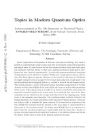
Figure 1: Photon number distribution of coherent (with an initial vacuum state |t = 0 =
|0 - solid curve) and semi-coherent states (with an initial one-photon state |t = 0 = |1
- dashed curve).
which then depends on the Fourier transform z = f(ω) =

∞
−∞
dtf(t) exp(−iωt).
In Figure 1, the solid curve gives P (n) for |φ
0
 = |0, where we, for the purpose
of illustration, have chosen the Fourier transform of f(t) such that the mean value
of the Poisson number-distribution of photons is |f(ω)|
2
= 49. The distribution
P (n) then characterize a classical state of the radiation field. The dashed curve in
Figure 1 corresponds to |φ
0
 = |1, and we observe the characteristic oscillations.
It may be a slight surprise that the minor change of the initial state by one photon

completely change the final distribution P (n) of photons, i.e. one photon among a
large number of photons (in the present case 49) makes a difference. If |φ
0
 = |m
one finds in the same way that the P (n)-distribution will have m zeros. If we sum
the distribution P (n) over the initial-state quantum number m we, of course, obtain
unity as a consequence of the unitarity of the time-evolution. Unitarity is actually
the simple quantum-mechanical reason why oscillations in P (n) must be present.
We also observe that two canonical coherent states |t
I
are orthogonal if the initial-
state fiducial vectors are orthogonal. It is in the sense of oscillations in P (n), as
described above, that a classical current can amplify a quantum-mechanical pure
state |φ
0
 to a coherent-state with a large number of coherent photons. This effect
is, of course, due to the boson character of photons.
It has, furthermore, been shown that one-photon states localized in space and
5
time can be generated in the laboratory (see e.g. [35]-[45]). It would be interesting
if such a state could be amplified by means of a classical source in resonance with
the typical frequency of the photon. It has been argued by Knight et al. [29] that
an imperfect photon-detection by allowing for dissipation of field-energy does not
necessarily destroy the appearance of the oscillations in the probability distribution
P (n) of photons in the displaced number-operator eigenstates. It would, of course,
be an interesting and striking verification of quantum coherence if the oscillations
in the P(n)-distribution could be observed experimentally.
3 Photon-Detection Theory
“If it was so, it might be; And if it were so,
it would be. But as it isn’t, it ain’t. ”

Lewis Carrol
The quantum-mechanical description of optical coherence was developed in a
series of beautiful papers by Glauber [14]. Here we will only touch upon some
elementary considerations of photo-detection theory. Consider an experimental sit-
uation where a beam of particles, in our case a beam of photons, hits an ideal
beam-splitter. Two photon-multipliers measures the corresponding intensities at
times t and t + τ of the two beams generated by the beam-splitter. The quantum
state describing the detection of one photon at time t and another one at time
t + τ is then of the form E
+
(t + τ )E
+
(t)|i, where |i describes the initial state and
where E
+
(t) denotes a positive-frequency component of the second-quantized elec-
tric field. The quantum-mechanical amplitude for the detection of a final state |f
then is f|E
+
(t + τ)E
+
(t)|i. The total detection-probability, obtained by summing
over all final states, is then proportional to the second-order correlation function
g
(2)
(τ) given by
g
(2)
(τ) =


f
|f|E
+
(t + τ)E
+
(t)|i|
2
(i|E
−
(t)E
+
(t)|i)
2
)
=
i|E
−
(t)E
−
(t + τ)E
+
(t + τ)E
+
(t)|i
(i|E
−
(t)E
+
(t)|i)
2

.
(3.1)
Here the normalization factor is just proportional to the intensity of the source, i.e.

f
|f|E
+
(t)|i|
2
= (i|E
−
(t)E
+
(t)|i)
2
. A classical treatment of the radiation field
would then lead to
g
(2)
(0) = 1 +
1
I
2

dIP (I)(I −I)
2
, (3.2)
where I is the intensity of the radiation field and P (I) is a quasi-probability distribu-
tion (i.e. not in general an apriori positive definite function). What we call classical
coherent light can then be described in terms of Glauber-Klauder coherent states.

These states leads to P (I) = δ(I −I). As long as P (I) is a positive definite func-
tion, there is a complete equivalence between the classical theory of optical coherence
6
and the quantum field-theoretical description [15]. Incoherent light, as thermal light,
leads to a second-order correlation function g
(2)
(τ) which is larger than one. This
feature is referred to as photon bunching (see e.g. Ref.[46]). Quantum-mechanical
light is, however, described by a second-order correlation function which may be
smaller than one. If the beam consists of N photons, all with the same quantum
numbers, we easily find that
g
(2)
(0) = 1 −
1
N
< 1 . (3.3)
Another way to express this form of photon anti-bunching is to say that in this
case the quasi-probability P (I) distribution cannot be positive, i.e. it cannot be
interpreted as a probability (for an account of the early history of anti-bunching see
e.g. Ref.[47, 48]).
3.1 Quantum Interference of Single Photons
A one-photon beam must, in particular, have the property that g
(2)
(0) = 0, which
simply corresponds to maximal photon anti-bunching. One would, perhaps, expect
that a sufficiently attenuated classical source of radiation, like the light from a pulsed
photo-diode or a laser, would exhibit photon maximal anti-bunching in a beam
splitter. This sort of reasoning is, in one way or another, explicitly assumed in many
of the beautiful tests of “single-photon” interference in quantum mechanics. It has,

however, been argued by Aspect and Grangier [49] that this reasoning is incorrect.
Aspect and Grangier actually measured the second-order correlation function g
(2)
(τ)
by making use of a beam-splitter and found this to be greater or equal to one even for
an attenuation of a classical light source below the one-photon level. The conclusion,
we guess, is that the radiation emitted from e.g. a monochromatic laser always
behaves in classical manner, i.e. even for such a strongly attenuated source below
the one-photon flux limit the corresponding radiation has no non-classical features
(under certain circumstances one can, of course, arrange for such an attenuated
light source with a very low probability for more than one-photon at a time (see
e.g. Refs.[50, 51]) but, nevertheless, the source can still be described in terms of
classical electro-magnetic fields). As already mentioned in the introduction, it is,
however, possible to generate photon beams which exhibit complete photon anti-
bunching. This has first been shown in the beautiful experimental work by Aspect
and Grangier [49] and by Mandel and collaborators [35]. Roger, Grangier and Aspect
in their beautiful study also verified that the one-photon states obtained exhibit
one-photon interference in accordance with the rules of quantum mechanics as we,
of course, expect. In the experiment by e.g. the Rochester group [35] beams of
one-photon states, localized in both space and time, were generated. A quantum-
mechanical description of such relativistic one-photon states will now be the subject
for Chapter 4.
7
3.2 Applications in High-Energy Physics
Many of the concepts from photon-detection theory has applications in the context
of high-energy physics. The use of photon-detection theory as mentioned in Sec-
tion 3 goes historically back to Hanbury-Brown and Twiss [52] in which case the
second-order correlation function was used in order to extract information on the
size of distant stars. The same idea has been applied in high-energy physics. The
two-particle correlation function C

2
(p
1
, p
2
), where p
1
and p
2
are three-momenta of
the (boson) particles considered, is in this case given by the ratio of two-particle
probabilities P (p
1
, p
2
) and the product of the one-particle probabilities P (p
1
) and
P (p
2
), i.e. C
2
(p
1
, p
2
) = P (p
1
, p
2

)/P (p
1
)P (p
2
). For a source of pions where any
phase-coherence is averaged out, corresponding to what is called a chaotic source,
there is an enhanced emission probability as compared to a non-chaotic source over
a range of momenta such that R|p
1
− p
2
|  1, where R represents an average of
the size of the pion source. For pions formed in a coherent-state one finds that
C
2
(p
1
, p
2
) = 1. The width of the experimentally determined correlation function of
pions with different momenta, i.e. C
2
(p
1
, p
2
), can therefore give information about
the size of the pion-source. A lot of experimental data has been compiled over the
years and the subject has recently been discussed in detail by e.g. Boal et al. [53]. A
recent experimental analysis has been considered by the OPAL collaboration in the

case of like-sign charged track pairs at a center-off-mass energy close to the Z
0
peak.
146624 multi-hadronic Z
0
candidates were used leading to an estimate of the radius
of the pion source to be close to one fermi [54]. Similarly the NA44 experiment at
CERN have studied π
+
π
+
-correlations from 227000 reconstructed pairs in S + P b
collisions at 200 GeV/c per nucleon leading to a space-time averaged pion-source
radius of the order of a few fermi [55]. The impressive experimental data and its
interpretation has been confronted by simulations using relativistic molecular dy-
namics [56]. In heavy-ion physics the measurement of the second-order correlation
function of pions is of special interest since it can give us information about the
spatial extent of the quark-gluon plasma phase, if it is formed. It has been sug-
gested that one may make use of photons instead of pions when studying possible
signals from the quark-gluon plasma. In particular, it has been suggested [57] that
the correlation of high transverse-momentum photons is sensitive to the details of
the space-time evolution of the high density quark-gluon plasma.
4 Relativistic Quantum Mechanics of Single Pho-
tons
“Because the word photon is used in so many ways,
it is a source of much confusion. The reader always
has to figure out what the writer has in mind.”
P. Meystre and M. Sargent III
8
The concept of a photon has a long and intriguing history in physics. It is, e.g.,

in this context interesting to notice a remark by A. Einstein; “All these fifty years of
pondering have not brought me any closer to answering the question: What are light
quanta? ” [58]. Linguistic considerations do not appear to enlighten our conceptual
understanding of this fundamental concept either [59]. Recently, it has even been
suggested that one should not make use of the concept of a photon at all [60]. As we
have remarked above, single photons can, however, be generated in the laboratory
and the wave-function of single photons can actually be measured [61]. The decay
of a single photon quantum-mechanical state in a resonant cavity has also recently
been studied experimentally [62].
A related concept is that of localization of relativistic elementary systems, which
also has a long and intriguing history (see e.g. Refs. [63]-[69]). Observations of
physical phenomena takes place in space and time. The notion of localizability of
particles, elementary or not, then refers to the empirical fact that particles, at a
given instance of time, appear to be localizable in the physical space.
In the realm of non-relativistic quantum mechanics the concept of localizability of
particles is built into the theory at a very fundamental level and is expressed in terms
of the fundamental canonical commutation relation between a position operator
and the corresponding generator of translations, i.e. the canonical momentum of a
particle. In relativistic theories the concept of localizability of physical systems is
deeply connected to our notion of space-time, the arena of physical phenomena, as a
4-dimensional continuum. In the context of the classical theory of general relativity
the localization of light rays in space-time is e.g. a fundamental ingredient. In fact,
it has been argued [70] that the Riemannian metric is basically determined by basic
properties of light propagation.
In a fundamental paper by Newton and Wigner [63] it was argued that in the
context of relativistic quantum mechanics a notion of point-like localization of a
single particle can be, uniquely, determined by kinematics. Wightman [64] extended
this notion to localization to finite domains of space and it was, rigorously, shown
that massive particles are always localizable if they are elementary, i.e. if they
are described in terms of irreducible representations of the Poincar´e group [71].

Massless elementary systems with non-zero helicity, like a gluon, graviton, neutrino
or a photon, are not localizable in the sense of Wightman. The axioms used by
Wightman can, of course, be weakened. It was actually shown by Jauch, Piron
and Amrein [65] that in such a sense the photon is weakly localizable. As will be
argued below, the notion of weak localizability essentially corresponds to allowing
for non-commuting observables in order to characterize the localization of massless
and spinning particles in general.
Localization of relativistic particles, at a fixed time, as alluded to above, has
been shown to be incompatible with a natural notion of (Einstein-) causality [72].
If relativistic elementary system has an exponentially small tail outside a finite
domain of localization at t = 0, then, according to the hypothesis of a weaker form
of causality, this should remain true at later times, i.e. the tail should only be
9
shifted further out to infinity. As was shown by Hegerfeldt [73], even this notion of
causality is incompatible with the notion of a positive and bounded observable whose
expectation value gives the probability to a find a particle inside a finite domain of
space at a given instant of time. It has been argued that the use of local observables
in the context of relativistic quantum field theories does not lead to such apparent
difficulties with Einstein causality [74].
We will now reconsider some of these questions related to the concept of local-
izability in terms of a quantum mechanical description of a massless particle with
given helicity λ [75, 76, 77] (for a related construction see Ref.[78]). The one-particle
states we are considering are, of course, nothing else than the positive energy one-
particle states of quantum field theory. We simply endow such states with a set of
appropriately defined quantum-mechanical observables and, in terms of these, we
construct the generators of the Poincar´e group. We will then show how one can
extend this description to include both positive and negative helicities, i.e. includ-
ing reducible representations of the Poincar´e group. We are then in the position to
e.g. study the motion of a linearly polarized photon in the framework of relativistic
quantum mechanics and the appearance of non-trivial phases of wave-functions.

4.1 Position Operators for Massless Particles
It is easy to show that the components of the position operators for a massless
particle must be non-commuting
1
if the helicity λ = 0. If J
k
are the generators
of rotations and p
k
the diagonal momentum operators, k = 1, 2, 3, then we should
have J · p = ±λ for a massless particle like the photon (see e.g. Ref.[79]). Here
J = (J
1
, J
2
, J
3
) and p = (p
1
, p
2
, p
3
). In terms of natural units (¯h = c = 1) we then
have that
[J
k
, p
l
] = i

klm
p
m
. (4.1)
If a canonical position operator x exists with components x
k
such that
[x
k
, x
l
] = 0 , (4.2)
[x
k
, p
l
] = iδ
kl
, (4.3)
[J
k
, x
l
] = i
klm
x
m
, (4.4)
then we can define generators of orbital angular momentum in the conventional way,
i.e.

L
k
= 
klm
x
l
p
m
. (4.5)
Generators of spin are then defined by
S
k
= J
k
−L
k
. (4.6)
They fulfill the correct algebra, i.e.
[S
k
, S
l
] = i
klm
S
m
, (4.7)
1
This argument has, as far as we know, first been suggested by N. Mukunda.
10

and they, furthermore, commute with x and p. Then, however, the spectrum of
S · p is λ, λ − 1, , −λ, which contradicts the requirement J · p = ±λ since, by
construction, J · p = S · p.
As has been discussed in detail in the literature, the non-zero commutator of
the components of the position operator for a massless particle primarily emerges
due to the non-trivial topology of the momentum space [75, 76, 77]. The irreducible
representations of the Poincar´e group for massless particles [71] can be constructed
from a knowledge of the little group G of a light-like momentum four-vector p =
(p
0
, p) . This group is the Euclidean group E(2). Physically, we are interested in
possible finite-dimensional representations of the covering of this little group. We
therefore restrict ourselves to the compact subgroup, i.e. we represent the E(2)-
translations trivially and consider G = SO(2) = U(1). Since the origin in the
momentum space is excluded for massless particles one is therefore led to consider
appropriate G-bundles over S
2
since the energy of the particle can be kept fixed.
Such G-bundles are classified by mappings from the equator to G, i.e. by the first
homotopy group Π
1
(U(1))=Z, where it turns out that each integer corresponds to
twice the helicity of the particle. A massless particle with helicity λ and sharp
momentum is thus described in terms of a non-trivial line bundle characterized by
Π
1
(U(1)) = {2λ} [80].
This consideration can easily be extended to higher space-time dimensions [77]. If
D is the number of space-time dimensions, the corresponding G-bundles are classified
by the homotopy groups Π

D−3
(Spin(D−2)). These homotopy groups are in general
non-trivial. It is a remarkable fact that the only trivial homotopy groups of this form
in higher space-time dimensions correspond to D = 5 and D = 9 due to the existence
of quaternions and the Cayley numbers (see e.g. Ref. [81]). In these space-time
dimensions, and for D = 3, it then turns that one can explicitly construct canonical
and commuting position operators for massless particles [77]. The mathematical fact
that the spheres S
1
, S
3
and S
7
are parallelizable can then be expressed in terms of
the existence of canonical and commuting position operators for massless spinning
particles in D = 3, D = 5 and D = 9 space-time dimensions.
In terms of a canonical momentum p
i
and coordinates x
j
satisfying the canonical
commutation relation Eq.(4.3) we can easily derive the commutator of two compo-
nents of the position operator x by making use of a simple consistency argument as
follows. If the massless particle has a given helicity λ, then the generators of angular
momentum is given by:
J
k
= 
klm
x

l
p
m
+ λ
p
k
|p|
. (4.8)
The canonical momentum then transforms as a vector under rotations, i.e.
[J
k
, p
l
] = i
klm
p
m
, (4.9)
without any condition on the commutator of two components of the position oper-
ator x. The position operator will, however, not transform like a vector unless the
11
following commutator is postulated
i[x
k
, x
l
] = λ
klm
p
m

|p|
3
, (4.10)
where we notice that commutator formally corresponds to a point-like Dirac mag-
netic monopole [82] localized at the origin in momentum space with strength 4πλ.
The energy p
0
of the massless particle is, of course, given by ω = |p|. In terms of a
singular U(1) connection A
l
≡ A
l
(p) we can write
x
k
= i∂
k
− A
k
, (4.11)
where ∂
k
= ∂/∂p
k
and
∂
k
A
l
− ∂

l
A
k
= λ
klm
p
m
|p|
3
. (4.12)
Out of the observables x
k
and the energy ω one can easily construct the generators
(at time t = 0) of Lorentz boots, i.e.
K
m
= (x
m
ω + ωx
m
)/2 , (4.13)
and verify that J
l
and K
m
lead to a realization of the Lie algebra of the Lorentz
group, i.e.
[J
k
, J

l
] = i
klm
J
m
, (4.14)
[J
k
, K
l
] = i
klm
K
m
, (4.15)
[K
k
, K
l
] = −i
klm
J
m
. (4.16)
The components of the Pauli-Plebanski operator W
µ
are given by
W
µ
= (W

0
, W) = (J · p, Jp
0
+ K ×p) = λp
µ
, (4.17)
i.e. we also obtain an irreducible representation of the Poincar´e group. The addi-
tional non-zero commutators are
[K
k
, ω] = ip
k
, (4.18)
[K
k
, p
l
] = iδ
kl
ω . (4.19)
At t ≡ x
0
(τ) = 0 the Lorentz boost generators K
m
as given by Eq.(4.13) are extended
to
K
m
= (x
m

ω + ωx
m
)/2 − tp
m
. (4.20)
In the Heisenberg picture, the quantum equation of motion of an observable O(t) is
obtained by using
dO(t)
dt
=
∂O(t)
∂t
+ i[H, O(t)] , (4.21)
12
where the Hamiltonian H is given by the ω. One then finds that all generators of
the Poincar´e group are conserved as they should. The equation of motion for x(t)
is
d
dt
x(t) =
p
ω
, (4.22)
which is an expected equation of motion for a massless particle.
The non-commuting components x
k
of the position operator x transform as the
components of a vector under spatial rotations. Under Lorentz boost we find in
addition that
i[K

k
, x
l
] =
1
2

x
k
p
l
ω
+
p
l
ω
x
k

− tδ
kl
+ λ
klm
p
m
|p|
2
. (4.23)
The first two terms in Eq.(4.23) corresponds to the correct limit for λ = 0 since
the proper-time condition x

0
(τ) ≈ τ is not Lorentz invariant (see e.g. [6], Section
2-9). The last term in Eq.(4.23) is due to the non-zero commutator Eq.(4.10). This
anomalous term can be dealt with by introducing an appropriate two-cocycle for
finite transformations consisting of translations generated by the position operator
x, rotations generated by J and Lorentz boost generated by K. For pure translations
this two-cocycle will be explicitly constructed in Section 4.3.
The algebra discussed above can be extended in a rather straightforward manner
to incorporate both positive and negative helicities needed in order to describe lin-
early polarized light. As we now will see this extension corresponds to a replacement
of the Dirac monopole at the origin in momentum space with a SU(2) Wu-Yang [83]
monopole. The procedure below follows a rather standard method of imbedding the
singular U(1) connection A
l
into a regular SU(2) connection. Let us specifically con-
sider a massless, spin-one particle. The Hilbert space, H, of one-particle transverse
wave-functions φ
α
(p), α = 1, 2, 3 is defined in terms of a scalar product
(φ, ψ) =

d
3
pφ
∗
α
(p)ψ
α
(p) , (4.24)
where φ

∗
α
(p) denotes the complex conjugated φ
α
(p). In terms of a Wu-Yang con-
nection A
a
k
≡ A
a
k
(p), i.e.
A
a
k
(p) = 
alk
p
l
|p|
2
, (4.25)
Eq.(4.11) is extended to
x
k
= i∂
k
− A
a
k

(p)S
a
, (4.26)
where
(S
a
)
kl
= −i
akl
(4.27)
are the spin-one generators. By means of a singular gauge-transformation the Wu-
Yang connection can be transformed into the singular U(1)-connection A
l
times
the third component of the spin generators S
3
(see e.g. Ref.[89]). This position
operator defined by Eq.(4.26) is compatible with the transversality condition on the
13
one-particle wave-functions, i.e. x
k
φ
α
(p) is transverse. With suitable conditions on
the one-particle wave-functions, the position operator x therefore has a well-defined
action on H. Furthermore,
i[x
k
, x

l
] = F
a
kl
S
a
= 
klm
p
m
|p|
3
ˆ
p · S , (4.28)
where
F
a
kl
= ∂
k
A
a
l
− ∂
l
A
a
k
− 
abc

A
b
k
A
c
l
= 
klm
p
m
p
a
|p|
4
, (4.29)
is the non-Abelian SU(2) field strength tensor and
ˆ
p is a unit vector in the direction
of the particle momentum p. The generators of angular momentum are now defined
as follows
J
k
= 
klm
x
l
p
m
+
p

k
|p|
ˆ
p · S . (4.30)
The helicity operator Σ ≡
ˆ
p · S is covariantly constant, i.e.
∂
k
Σ + i [A
k
, Σ] = 0 , (4.31)
where A
k
≡ A
a
k
(p)S
a
. The position operator x therefore commutes with
ˆ
p ·S. One
can therefore verify in a straightforward manner that the observables p
k
, ω, J
l
and
K
m
= (x

m
ω + ωx
m
)/2 close to the Poincar´e group. At t = 0 the Lorentz boost
generators K
m
are defined as in Eq.(4.20) and Eq.(4.23) is extended to
i[K
k
, x
l
] =
1
2

x
k
p
l
ω
+
p
l
ω
x
k

− tδ
kl
+ iω[x

k
, x
l
] . (4.32)
For helicities
ˆ
p·S = ±λ one extends the previous considerations by considering S
in the spin |λ|-representation. Eqs.(4.28), (4.30) and (4.32) are then valid in general.
A reducible representation for the generators of the Poincar´e group for an arbitrary
spin has therefore been constructed for a massless particle. We observe that the
helicity operator Σ can be interpreted as a generalized “magnetic charge”, and since
Σ is covariantly conserved one can use the general theory of topological quantum
numbers [84] and derive the quantization condition
exp(i4πΣ) = 1 , (4.33)
i.e. the helicity is properly quantized. In the next section we will present an alter-
native way to derive helicity quantization.
4.2 Wess-Zumino Actions and Topological Spin
Coadjoint orbits on a group G has a geometrical structure which naturally admits a
symplectic two-form (see e.g. [85, 86, 87]) which can be used to construct topological
Lagrangians, i.e. Lagrangians constructed by means of Wess-Zumino terms [88] (for
a general account see e.g. Refs.[89, 90]). Let us illustrate the basic ideas for a
14
non-relativistic spin and G = SU(2). Let K be an element of the Lie algebra G
of G in the fundamental representation. Without loss of generality we can write
K = λ
α
σ
α
= λσ
3

, where σ
α
, α = 1, 2, 3 denotes the three Pauli spin matrices. Let H
be the little group of K. Then the coset space G/H is isomorphic to S
2
and defines
an adjoint orbit (for semi-simple Lie groups adjoint and coadjoint representations
are equivalent due to the existence of the non-degenerate Cartan-Killing form). The
action for the spin degrees of freedom is then expressed in terms of the group G
itself, i.e.
S
P
= −i


K, g
−1
(τ)dg(τ )/dτ

dτ , (4.34)
where A, B denotes the trace-operation of two Lie-algebra elements A and B in G
and where
g(τ ) = exp(iσ
α
ξ
α
(τ)) (4.35)
defines the (proper-)time dependent dynamical group element. We observe that S
P
has a gauge-invariance, i.e. the transformation

g(τ ) −→ g(τ ) exp (iθ(τ )σ
3
) (4.36)
only change the Lagrangian density K, g
−1
(τ)dg(τ )/dτ  by a total time derivative.
The gauge-invariant components of spin, S
k
(τ), are defined in terms of K by the
relation
S(τ) ≡ S
k
(τ)σ
k
= λg(τ )σ
3
g
−1
(τ) , (4.37)
such that
S
2
≡ S
k
(τ)S
k
(τ) = λ
2
. (4.38)
By adding a non-relativistic particle kinetic term as well as a conventional magnetic

moment interaction term to the action S
P
, one can verify that the components S
k
(τ)
obey the correct classical equations of motion for spin-precession [75, 89].
Let M = {σ, τ|σ ∈ [0, 1]} and (σ, τ) → g(σ, τ) parameterize τ−dependent paths
in G such that g(0, τ ) = g
0
is an arbitrary reference element and g(1, τ ) = g(τ ). The
Wess-Zumino term in this case is given by
ω
W Z
= −id

K, g
−1
(σ, τ)dg(σ, τ)

= i

K, (g
−1
(σ, τ)dg(σ, τ))
2

, (4.39)
where d denotes exterior differentiation and where now
g(σ, τ) = exp(iσ
α

ξ
α
(σ, τ)) . (4.40)
Apart from boundary terms which do not contribute to the equations of motion, we
then have that
S
P
= S
W Z
≡

M
ω
W Z
= −i

∂M

K, g
−1
(τ)dg(τ )

, (4.41)
where the one-dimensional boundary ∂M of M , parameterized by τ , can play the
role of (proper-) time. ω
W Z
is now gauge-invariant under a larger U(1) symmetry,
i.e. Eq.(4.36) is now extended to
g(σ, τ) −→ g(σ, τ) exp (iθ(σ, τ)σ
3

) . (4.42)
15
ω
W Z
is therefore a closed but not exact two-form defined on the coset space G/H. A
canonical analysis then shows that there are no gauge-invariant dynamical degrees of
freedom in the interior of M. The Wess-Zumino action Eq.(4.41) is the topological
action for spin degrees of freedom.
As for the quantization of the theory described by the action Eq.(4.41), one
may use methods from geometrical quantization and especially the Borel-Weil-Bott
theory of representations of compact Lie groups [85, 89]. One then finds that λ
is half an integer, i.e. |λ| corresponds to the spin. This quantization of λ also
naturally emerges by demanding that the action Eq.(4.41) is well-defined in quantum
mechanics for periodic motion as recently was discussed by e.g. Klauder [91], i.e.
4πλ =

S
2
ω
W Z
= 2πn , (4.43)
where n is an integer. The symplectic two-form ω
W Z
must then belong to an in-
teger class cohomology. This geometrical approach is in principal straightforward,
but it requires explicit coordinates on G/H. An alternative approach, as used in
[75, 89], is a canonical Dirac analysis and quantization [6]. This procedure leads to
the condition λ
2
= s(s + 1), where s is half an integer. The fact that one can arrive

at different answers for λ illustrates a certain lack of uniqueness in the quantization
procedure of the action Eq.(4.41). The quantum theories obtained describes, how-
ever, the same physical system namely one irreducible representation of the group
G.
The action Eq.(4.41) was first proposed in [92]. The action can be derived quite
naturally in terms of a coherent state path integral (for a review see e.g. Ref.[7])
using spin coherent states. It is interesting to notice that structure of the action
Eq.(4.41) actually appears in such a language already in a paper by Klauder on
continuous representation theory [93].
A classical action which after quantization leads to a description of a massless
particle in terms of an irreducible representations of the Poincar´e group can be
constructed in a similar fashion [75]. Since the Poincar´e group is non-compact the
geometrical analysis referred to above for non-relativistic spin must be extended and
one should consider coadjoint orbits instead of adjoint orbits (D=3 appears to be
an exceptional case due to the existence of a non-degenerate bilinear form on the
D=3 Poincar´e group Lie algebra [94]. In this case there is a topological action for
irreducible representations of the form Eq.(4.41) [95]). The point-particle action in
D=4 then takes the form
S =

dτ

p
µ
(τ) ˙x
µ
(τ) +
i
2
Tr[KΛ

−1
(τ)
d
dτ
Λ(τ)]

. (4.44)
Here [σ
αβ
]
µν
= −i(η
αµ
η
βν
−η
αν
η
βµ
) are the Lorentz group generators in the spin-one
representation and η
µν
= (−1, 1, 1, 1) is the Minkowski metric. The trace operation
has a conventional meaning, i.e. Tr[M] = M
α
α
. The Lorentz group Lie-algebra
element K is here chosen to be λσ
12
. The τ -dependence of the Lorentz group element

16
Λ
µν
(τ) is defined by
Λ
µν
(τ) =

exp

iσ
αβ
ξ
αβ
(τ)

µν
. (4.45)
The momentum variable p
µ
(τ) is defined by
p
µ
(τ) = Λ
µν
(τ)k
ν
, (4.46)
where the constant reference momentum k
ν

is given by
k
ν
= (ω, 0, 0, |k|) , (4.47)
where ω = |k|. The momentum p
µ
(τ) is then light-like by construction. The action
Eq.(4.44) leads to the equations of motion
d
dτ
p
µ
(τ) = 0 , (4.48)
and
d
dτ

x
µ
(τ)p
ν
(τ) −x
ν
(τ)p
µ
(τ) + S
µν
(τ)

= 0 . (4.49)

Here we have defined gauge-invariant spin degrees of freedom S
µν
(τ) by
S
µν
(τ) =
1
2
Tr[Λ(τ )KΛ
−1
(τ)σ
µν
] (4.50)
in analogy with Eq.(4.37). These spin degrees of freedom satisfy the relations
p
µ
(τ)S
µν
(τ) = 0 , (4.51)
and
1
2
S
µν
(τ)S
µν
(τ) = λ
2
. (4.52)
Inclusion of external electro-magnetic and gravitational fields leads to the classical

Bargmann-Michel-Telegdi [96] and Papapetrou [97] equations of motion respectively
[75]. Since the equations derived are expressed in terms of bosonic variables these
equations of motion admit a straightforward classical interpretation. (An alternative
bosonic or fermionic treatment of internal degrees of freedom which also leads to
Wongs equations of motion [98] in the presence of in general non-Abelian external
gauge fields can be found in Ref.[99].)
Canonical quantization of the system described by bosonic degrees of freedom
and the action Eq.(4.44) leads to a realization of the Poincar´e Lie algebra with
generators p
µ
and J
µν
where
J
µν
= x
µ
p
ν
− x
ν
p
µ
+ S
µν
. (4.53)
17
The four vectors x
µ
and p

ν
commute with the spin generators S
µν
and are canonical,
i.e.
[x
µ
, x
ν
] = [p
µ
, p
ν
] = 0 , (4.54)
[x
µ
, p
ν
] = iη
µν
. (4.55)
The spin generators S
µν
fulfill the conventional algebra
[S
µν
, S
λρ
] = i(η
µλ

S
νρ
+ η
νρ
S
µλ
− η
µρ
S
νλ
−η
νλ
S
µρ
) . (4.56)
The mass-shell condition p
2
= 0 as well as the constraints Eq.(4.51) and Eq.(4.52)
are all first-class constraints [6]. In the proper-time gauge x
0
(τ) ≈ τ one obtains
the system described in Section 4.1, i.e. we obtain an irreducible representation of
the Poincar´e group with helicity λ [75]. For half-integer helicity, i.e. for fermions,
one can verify in a straightforward manner that the wave-functions obtained change
with a minus-sign under a 2π rotation [75, 77, 89] as they should.
4.3 The Berry Phase for Single Photons
We have constructed a set of O(3)-covariant position operators of massless particles
and a reducible representation of the Poincar´e group corresponding to a combination
of positive and negative helicities. It is interesting to notice that the construction
above leads to observable effects. Let us specifically consider photons and the motion

of photons along e.g. an optical fibre. Berry has argued [100] that a spin in an
adiabatically changing magnetic field leads to the appearance of an observable phase
factor, called the Berry phase. It was suggested in Ref.[101] that a similar geometric
phase could appear for photons. We will now, within the framework of the relativistic
quantum mechanics of a single massless particle as discussed above, give a derivation
of this geometrical phase. The Berry phase for a single photon can e.g. be obtained
as follows. We consider the motion of a photon with fixed energy moving e.g. along
an optical fibre. We assume that as the photon moves in the fibre, the momentum
vector traces out a closed loop in momentum space on the constant energy surface,
i.e. on a two-sphere S
2
. This simply means that the initial and final momentum
vectors of the photon are the same. We therefore consider a wave-function |p which
is diagonal in momentum. We also define the translation operator U(a) = exp(ia·x).
It is straightforward to show, using Eq.(4.10), that
U(a)U(b) |p = exp(iγ[a, b; p]) |p + a + b , (4.57)
where the two-cocycle phase γ[a, b; p] is equal to the flux of the magnetic monopole
in momentum space through the simplex spanned by the vectors a and b localized
at the point p, i.e.
γ[a, b; p] = λ

1
0

1
0
dξ
1
dξ
2

a
k
b
l

lkm
B
m
(p + ξ
1
a + ξ
2
b) , (4.58)
18
where B
m
(p) = p
m
/|p|
3
. The non-trivial phase appears because the second de Rham
cohomology group of S
2
is non-trivial. The two-cocycle phase γ[a, b; p] is therefore
not a coboundary and hence it cannot be removed by a redefinition of U(a). This
result has a close analogy in the theory of magnetic monopoles [102]. The anomalous
commutator Eq.(4.10) therefore leads to a ray-representation of the translations in
momentum space.
A closed loop in momentum space, starting and ending at p, can then be obtained
by using a sequence of infinitesimal translations U(δa) |p = |p + δa such that δa

is orthogonal to argument of the wave-function on which it acts (this defines the
adiabatic transport of the system). The momentum vector p then traces out a closed
curve on the constant energy surface S
2
in momentum space. The total phase of
these translations then gives a phase γ which is the λ times the solid angle of the
closed curve the momentum vector traces out on the constant energy surface. This
phase does not depend on Plancks constant. This is precisely the Berry phase for the
photon with a given helicity λ. In the original experiment by Tomita and Chiao [103]
one considers a beam of linearly polarized photons (a single-photon experiment is
considered in Ref.[104]). The same line of arguments above but making use Eq.(4.28)
instead of Eq.(4.10) leads to the desired change of polarization as the photon moves
along the optical fibre.
A somewhat alternative derivation of the Berry phase for photons is based on
observation that the covariantly conserved helicity operator Σ can be interpreted as
a generalized “magnetic charge”. Let Γ denote a closed path in momentum space
parameterized by σ ∈ [0, 1] such that p(σ = 0) = p(σ = 1) = p
0
is fixed. The
parallel transport of a one-particle state φ
α
(p) along the path Γ is then determined
by a path-ordered exponential, i.e.
φ
α
(p
0
) −→

P exp


i

Γ
A
k
(p(σ))
dp
k
(σ)
dσ
dσ

αβ
φ
β
(p
0
) , (4.59)
where A
k
(p(σ)) ≡ A
a
k
(p(σ))S
a
. By making use of a non-Abelian version of Stokes
theorem [84] one can then show that
P exp


i

Γ
A
k
(p(σ))
dp
k
(σ)
dσ
dσ

= exp (iΣΩ[Γ]) , (4.60)
where Ω[Γ] is the solid angle subtended by the path Γ on the two-sphere S
2
. This
result leads again to the desired change of linear polarization as the photon moves
along the path described by Γ. Eq.(4.60) also directly leads to helicity quantiza-
tion, as alluded to already in Section 4.1, by considering a sequence of loops which
converges to a point and at the same time has covered a solid angle of 4π. This
derivation does not require that |p(σ)| is constant along the path.
In the experiment of Ref.[103] the photon flux is large. In order to strictly apply
our results under such conditions one can consider a second quantized version of the
theory we have presented following e.g. the discussion of Amrein [65]. By making
19
use of coherent states of the electro-magnetic field in a standard and straightforward
manner (see e.g. Ref.[7]) one then realize that our considerations survive. This is
so since the coherent states are parameterized in terms of the one-particle states.
By construction the coherent states then inherits the transformation properties of
the one-particle states discussed above. It is, of course, of vital importance that the

Berry phase of single-photon states has experimentally been observed [104].
4.4 Localization of Single-Photon States
In this section we will see that the fact that a one-photon state has positive energy,
generically makes a localized one-photon wave-packet de-localized in space in the
course of its time-evolution. We will, for reasons of simplicity, restrict ourselves
to a one-dimensional motion, i.e. we have assume that the transverse dimensions
of the propagating localized one-photon state are much large than the longitudinal
scale. We will also neglect the effect of photon polarization. Details of a more
general treatment can be found in Ref.[105]. In one dimension we have seen above
that the conventional notion of a position operator makes sense for a single photon.
We can therefore consider wave-packets not only in momentum space but also in
the longitudinal co-ordinate space in a conventional quantum-mechanical manner.
One can easily address the same issue in terms of photon-detection theory but in
the end no essential differences will emerge. In the Sch¨odinger picture we are then
considering the following initial value problem (c = ¯h = 1)
i
∂ψ(x, t)
∂t
=

−
d
2
dx
2
ψ(x, t) ,
ψ(x, 0) = exp(−x
2
/2a
2

) exp(ik
0
x) , (4.61)
which describes the unitary time-evolution of a single-photon wave-packet localized
within the distance a and with mean-momentum < p >= k
0
. The non-local pseudo-
differential operator

−d
2
/dx
2
is defined in terms of Fourier-transform techniques,
i.e.

−
d
2
dx
2
ψ(x) =

∞
−∞
dyK(x − y)ψ(y) , (4.62)
where the kernel K(x) is given by
K(x) =
1
2π


∞
−∞
dk|k|exp(ikx) . (4.63)
The co-ordinate wave function at any finite time can now easily be written down
and the probability density is shown in Figure 2 in the case of a non-zero average
momentum of the photon. The form of the soliton-like peaks is preserved for suffi-
ciently large times. In the limit of ak
0
= 0 one gets two soliton-like identical peaks
propagating in opposite directions. The structure of these peaks are actually very
similar to the directed localized energy pulses in Maxwells theory [106] or to the
20
-15
-10
-5
0
5
10
15
0
0.1
0.2
0.3
0.4
0.5
k
0
a = 0.5
P (x)

x/a
Figure 2: Probability density-distribution P(x) = |ψ(x, t)|
2
for a one-dimensional Gaus-
sian single-photon wave-packet with k
0
a = 0.5 at t = 0 (solid curve) and at t/a = 10
(dashed curve).
pulse splitting processes in non-linear dispersive media (see e.g. Ref.[107]) but the
physics is, of course, completely different.
Since the wave-equation Eq.(4.61) leads to the second-order wave-equation in
one-dimension the physics so obtained can, of course, be described in terms of solu-
tions to the one-dimensional d’Alembert wave-equation of Maxwells theory of elec-
tromagnetism. The quantum-mechanical wave-function above in momentum space
is then simply used to parameterize a coherent state. The average of a second-
quantized electro-magnetic free field operator in such a coherent state will then be
a solution of this wave-equation. The solution to the d’Alembertian wave-equation
can then be written in terms of the general d’Alembertian formula, i.e.
ψ
cl
(x, t) =
1
2
(ψ(x + t, 0)+ ψ(x −t, 0)) +
1
2i

x+t
x−t
dy


∞
−∞
dzK(y −z)ψ(z, 0) , (4.64)
where the last term corresponds to the initial value of the time-derivative of the
classical electro-magnetic field. The fact this term is non-locally connected to the
initial value of the classical electro-magnetic field is perhaps somewhat unusual. By
construction ψ
cl
(x, t) = ψ(x, t). The physical interpretation of the two functions
ψ(x, t) and ψ
cl
(x, t) are, of course, very different. In the quantum-mechanical case
the detection of the photon destroys the coherence properties of the wave-packet
21
ψ(x, t) entirely. In the classical case the detection of a single photon can still preserve
the coherence properties of the classical field ψ
cl
(x, t) since there are infinitely many
photons present in the corresponding coherent state.
4.5 Various Comments
In the analysis of Wightman, corresponding to commuting position variables, the
natural mathematical tool turned out to be systems of imprimitivity for the repre-
sentations of the three-dimensional Euclidean group. In the case of non-commuting
position operators we have also seen that notions from differential geometry are im-
portant. It is interesting to see that such a broad range of mathematical methods
enters into the study of the notion of localizability of physical systems.
We have, in particular, argued that Abelian as well as non-Abelian magnetic
monopole field configurations reveal themselves in a description of localizability of
massless spinning particles. Concerning the physical existence of magnetic monopoles

Dirac remarked in 1981 [108] that “I am inclined now to believe that monopoles do
not exist. So many years have gone by without any encouragement from the experi-
mental side”. The “monopoles” we are considering are, however, only mathematical
objects in the momentum space of the massless particles. Their existence, we have
argued, is then only indirectly revealed to us by the properties of e.g. the photons
moving along optical fibres.
Localized states of massless particles will necessarily develop non-exponential
tails in space as a consequence of the Hegerfeldts theorem [73]. Various number op-
erators representing the number of massless, spinning particles localized in a finite
volume V at time t has been discussed in the literature. The non-commuting po-
sition observables we have discussed for photons correspond to the point-like limit
of the weak localizability of Jauch, Piron and Amrein [65]. This is so since our
construction, as we have seen in Section 4.1, corresponds to an explicit enforcement
of the transversality condition of the one-particle wave-functions.
In a finite volume, photon number operators appropriate for weak localization
[65] do not agree with the photon number operator introduced by Mandel [109] for
sufficiently small wavelengths as compared to the linear dimension of the localiza-
tion volume. It would be interesting to see if there are measurable differences. A
necessary ingredient in answering such a question would be the experimental real-
ization of a localized one-photon state. It is interesting to notice that such states
can be generated in the laboratory [35]-[45].
As a final remark of this first set of lectures we recall a statement of Wightman
which, to a large extent, still is true [64]: “Whether, in fact, the position of such
particle is observable in the sense of quantum theory is, of course, a much deeper
problem that probably can only be be decided within the context of a specific conse-
quent dynamical theory of particles. All investigations of localizability for relativistic
particles up to now, including the present one, must be regarded as preliminary from
this point of view: They construct position observables consistent with a given trans-
22