Agricultural nonpoint source pollution
Bạn đang xem bản rút gọn của tài liệu. Xem và tải ngay bản đầy đủ của tài liệu tại đây (8.88 MB, 331 trang )
LEWIS PUBLISHERS
Boca Raton London New York Washington, D.C.
AGRICULTURAL
NONPOINT
SOURCE
POLLUTION
Edited by
Watershed Management
and Hydrology
William F. Ritter
Adel Shirmohammadi
© 2001 by CRC Press LLC
This book contains information obtained from authentic and highly regarded sources. Reprinted material
is quoted with permission, and sources are indicated. A wide variety of references are listed. Reasonable
efforts have been made to publish reliable data and information, but the author and the publisher cannot
assume responsibility for the validity of all materials or for the consequences of their use.
Neither this book nor any part may be reproduced or transmitted in any form or by any means, electronic
or mechanical, including photocopying, microfilming, and recording, or by any information storage or
retrieval system, without prior permission in writing from the publisher.
All rights reserved. Authorization to photocopy items for internal or personal use, or the personal or
internal use of specific clients, may be granted by CRC Press LLC, provided that $.50 per page
photocopied is paid directly to Copyright Clearance Center, 222 Rosewood Drive, Danvers, MA 01923
USA. The fee code for users of the Transactional Reporting Service is ISBN 0-1-56670-222-
4/01/$0.00+$.50. The fee is subject to change without notice. For organizations that have been granted
a photocopy license by the CCC, a separate system of payment has been arranged.
The consent of CRC Press LLC does not extend to copying for general distribution, for promotion, for
creating new works, or for resale. Specific permission must be obtained in writing from CRC Press LLC
for such copying.
Direct all inquiries to CRC Press LLC, 2000 N.W. Corporate Blvd., Boca Raton, Florida 33431.
Trademark Notice: Product or corporate names may be trademarks or registered trademarks, and are
used only for identification and explanation, without intent to infringe.
© 2001 by CRC Press LLC
Lewis Publishers is an imprint of CRC Press LLC
No claim to original U.S. Government works
International Standard Book Number 1-56670-222-4
Library of Congress Card Number 0046349
Printed in the United States of America 1 2 3 4 5 6 7 8 9 0
Printed on acid-free paper
Library of Congress Cataloging-in-Publication Data
Agricultural nonpoint source pollution : watershed management and hydrology / edited
by William F. Ritter, Adel Shirmohammadi
p. cm.
Includes bibliographical references.
ISBN 1-56670-222-4 (alk. paper)
1. Agricultural pollution Environmental aspects United States. 2. Nonpoint source
pollution United States. 3.Watershed management United States. 4. Water quality
management United States. I. Ritter, William F. II. Shirmohammadi, Adel, 1952-
TD428.A37 A362 2000
628.1′.684—dc21 00-046349
CIP
© 2001 by CRC Press LLC
iii
Preface
Despite the tremendous progress that has been achieved in water pollution, almost
40% of the U.S. waters that have been assessed by states do not meet water quality
goals. About 20,000 water bodies are impacted by siltation, nutrients, bacteria, oxy-
gen depletion substances, metals, habitat alterations, pesticides, and toxic organic
chemicals. With pollution from point sources being dramatically reduced, nonpoint
source pollution is the major cause of most water that does not meet water quality
goals. About 50 to 70% of the assessed surface waters are adversely affected by agri-
cultural nonpoint source pollution caused by soil erosion from cropland and over-
grazing and from pesticide and fertilizer applications. States have identified almost
500,000 kilometers of rivers and streams and more than two million hectares of lakes
that do not meet state water quality goals. In 1998, about one-third of the 1062
beaches reporting to the U.S. Environmental Protection Agency had at least one
health advisory or closing. More than 2500 fish consumption advisories or bans were
issued by states in areas where fish were too contaminated to eat.
Clean water is important for the nation’s economy. A third of Americans visit
coastal areas each year, generating new jobs and billions of dollars. Closed beaches
and fish advisories result in lost revenue. Water used for irrigating crops and raising
livestock helps American farmers produce and sell $197 billion worth of food and
fiber each year. Manufacturers use thirty-five trillion liters of fresh water annually.
This book is intended to give a comprehensive overview of agricultural nonpoint
source pollution and its management on a watershed scale. The first chapter provides
background information on watershed hydrology, with a discussion on each phase of
the hydrologic cycle. The second chapter is on soil erosion and sedimentation. The
basic processes of soil erosion as it occurs in upland areas are discussed, most of it
focused on rill and interrill erosion. Process-based soil erosion models and cropping
and management effects on erosion are treated and contrasted in some detail.
Chapters 3, 4, and 5 take up the nonpoint source pollutants nitrogen, phospho-
rus, and pesticides in detail. Both surface and subsurface processes are discussed in
each chapter. Chapters 3 and 4 begin with nitrogen and phosphorus cycles, respec-
tively. Management practices to control nonpoint source pollution from nitrogen,
phosphorus, and pesticides are discussed.
Chapter 6 discusses nonpoint source pollution from the livestock industry.
Surface water and groundwater quality effects from feedlots, manure storage and
treatment systems, and land application of manures are presented, along with non-
point source pollution control practices for each of these sources.
Chapter 7 addresses the impact of irrigated agriculture on water quality.
The nonpoint source pollutants nitrates, pesticides, salts, trace elements, and sus-
pended sediments are discussed, along with management practices for reducing non-
point source pollution from irrigation. Chapter 8 is focused on the impact of
© 2001 by CRC Press LLC
agricultural drainage on water quality. Both conventional drainage and water-table
management are discussed.
Chapter 9 provides an overview of water quality models. Different types of water
quality models are discussed along with model development, sensitivity analysis,
model validation and verification, and the role of geographic information systems in
water quality modeling. Chapter 10 provides a treatment of best management prac-
tices (BMPs) to control nonpoint source pollution and the framework for the design
of a monitoring system for BMP impact assessment. Fourteen BMPs are discussed in
detail.
The final chapter discusses monitoring, including monitoring system design,
data needs and collection, and implementation strategies, along with methods to
monitor edge-of-field overland flow, bottom of root zone, soil, groundwater, and sur-
face water.
The editors thank all authors for their valuable contribution to this book. We
hope it will give people a better insight into the issues involved in agricultural non-
point source pollution and its control.
William F. Ritter
Adel Shirmohammadi
© 2001 by CRC Press LLC
v
Editors
William F. Ritter, Ph.D. is Professor of Bioresources and Civil and Environmental
Engineering at the University of Delaware and a Senior Policy Fellow in the Center
for Energy and Environment Policy.
In 1965 Dr. Ritter received his B.S.A. in agricultural engineering from the
University of Guelph, and in 1966 received a B.A.S. in civil engineering from the
University of Toronto. He obtained his M.S. in 1968 in water resources and his Ph.D.
in 1971 in sanitary and agricultural engineering from Iowa State University. He was
a research associate at Iowa State University from 1966 to 1971 and joined the
Agricultural Engineering Department at the University of Delaware as an assistant
professor in 1971. He served as department chair of the Agricultural Engineering
Department from 1992 to 1998.
Dr. Ritter is a registered professional engineer in Delaware, Maryland,
Pennsylvania, and New Jersey and is a fellow of the American Society of Agricultural
Engineers and American Society of Civil Engineers. He is also a member of the
American Water Works Association, Water Environment Federation, Canadian
Society of Agricultural Engineers, and American Society of Engineering Education.
He has taught courses on hydrology, soil erosion, irrigation, drainage, soil physics,
solid waste management, wastewater treatment, and land application of wastes. He
has conducted research on irrigation water management, livestock waste manage-
ment, surface and groundwater quality, and land application of wastes. He has served
as a consultant to government and industry on wastewater management, water qual-
ity, land application of wastes, and livestock waste management.
Dr. Ritter is the author of more than 270 papers, reports, and book contributions
and has presented over 140 papers at regional, national, and international confer-
ences. He has also received numerous awards that include the College of Agriculture
Outstanding Research Award (1990), ASAE Gunlogson Countryside Engineering
Award (1989), ASCE Outstanding News Correspondent (1997), and ASCE Delaware
Section Civil Engineer of the Year (1999).
Dr. Adel Shirmohammadi, Ph.D. is Professor of Biological Resources
Engineering at the University of Maryland, College Park campus.
In 1974, Dr. Shirmohammadi received his B.S. in agricultural engineering from
the University of Rezaeiyeh in Iran. He obtained an M.S. in 1977 in agricultural engi-
neering from the University of Nebraska and a Ph.D. in 1982 in biological and agri-
cultural engineering from North Carolina State University. From 1982 to 1986 he was
a post-doctoral agricultural research engineer and assistant research scientist in the
Agricultural Engineering Department at the University of Georgia Coastal Plains
Experiment Station at Tifton. In 1986, he joined the Agricultural Engineering
Department at the University of Maryland as an assistant professor.
Dr. Shirmohammadi is a member of the American Society of Agricultural
Engineers, Soil and Water Conservation Society of America, and American
© 2001 by CRC Press LLC
Geophysical Union. He has taught courses in hydrology, soil and water conservation
engineering, water quality modeling, flow-through porous media, and nonpoint
source pollution. He has conducted research in hydrologic and water quality mode-
ling, drainage, and nonpoint source pollution. He has developed an international
reputation in water quality modeling for his work with CREAMS, GLEAMS,
DRAINMODE, and ANSWERS.
Dr. Shirmohammadi has received numerous competitive grants and has served as
a consultant to industry and government. He is the author of more than 100 refereed
publications, conference proceedings, papers, and book contributions.
© 2001 by CRC Press LLC
,
Contributors
Lars Bergstrom, Ph.D.
Professor
Swedish University of Agricultural
Sciences
Division of Water Quality Research
Uppsala, Sweden
Kevin M. Brannan, M.S.
Research Associate
Biological Systems Engineering
Department
Virginia Polytechnic and State
University
Blacksburg, VA
Adriana C. Bruggeman, Ph.D.
Research Associate
Biological Systems Engineering
Department
Virginia Polytechnic and State
University
Blacksburg, VA
Kenneth L. Campbell, Ph.D.
Professor
Agricultural and Biological Engineering
Department
University of Florida
Gainesville, FL
Theo A. Dillaha III, Ph.D.
Professor
Biological Systems Engineering
Department
Virginia Polytechnic and State
University
Blacksburg, VA
Dwayne R. Edwards, Ph.D.
Associate Professor
Biosystems and Agricultural
Engineering Department
University of Kentucky
Lexington, KY
Blaine R. Hanson, Ph.D.
Irrigation and Drainage Specialist
Department of Land, Air and Water
Resources
University of California
Davis, CA
Walter G. Knisel, Jr., Ph.D.
Retired Hydraulic Engineer of USDA-
ARS and Affiliate Professor
Biological and Agricultural Engineering
Department
Coastal Plains Experiment Station
University of Georgia
Tifton, GA
© 2001 by CRC Press LLC
William L. Magette, Ph.D.
Lecturer
Agricultural and Food Engineering
Department
University College Dublin
Dublin, Ireland
Hubert J. Montas, Ph.D.
Assistant Professor
Biological Resources Engineering
Department
University of Maryland
College Park, MD
Saied Mostaghimi, Ph.D.
H. E. and Elizabeth Alphin Professor
Biological Systems Engineering
Department
Virginia Polytechnic and State
University
Blacksburg, VA
Mark A. Nearing, Ph.D.
Scientist
USDA-ARS National Soil Erosion
Research Laboratory
West Lafayette, IN
L. Darrell Norton, Ph.D.
Scientist
USDA-ARS National Soil Erosion
Research Laboratory
West Lafayette, IN
Adel Shirmohammadi, Ph.D.
Biological Resources Engineering
Department
University of Maryland
College Park, MD
William F. Ritter, Ph.D.
Bioresources Engineering
Department
University of Delaware
Newark, DE
Thomas J. Trout, Ph.D.
Agricultural Engineer
USDA-ARS Water Management
Research Laboratory
Fresno, CA
Mary Leigh Wolfe, Ph.D.
Associate Professor
Biological Systems Engineering
Department
Virginia Polytechnic and State
University
Blacksburg, VA
Xunchang Zhang, Ph.D.
Scientist
USDA-ARS Soil Erosion Research
Laboratory
West Lafayette, IN
© 2001 by CRC Press LLC
Table of Contents
Chapter 1
Hydrology
Mary Leigh Wolfe
Chapter 2
Soil Erosion and Sedimentation
Mark A. Nearing, L. Darrell Norton, and Xunchang Zhang
Chapter 3
Nitrogen and Water Quality
William F. Ritter and Lars Bergstrom
Chapter 4
Phosphorus and Water Quality Impacts
Kenneth L. Campbell and Dwayne R. Edwards
Chapter 5
Pesticides and Water Quality Impacts
William F. Ritter
Chapter 6
Nonpoint Source Pollution and Livestock Manure Management
William F. Ritter
Chapter 7
Irrigated Agriculture and Water Quality Impacts
Blaine R. Hanson and Thomas J. Trout
Chapter 8
Agricultural Drainage and Water Quality
William F. Ritter and Adel Shirmohammadi
Chapter 9
Water Quality Models
Adel Shirmohammadi, Hubert J. Montas, Lars Bergstrom, and Walter J. Knisel, Jr.
© 2001 by CRC Press LLC
Chapter 10
Best Management Practices for Nonpoint Source Pollution Control:
Selection and Assessment
Saied Mostaghimi, Kevin M. Brannan, Theo A. Dillaha and
Adriana C. Bruggeman
Chapter 11
Monitoring
William L. Magette
© 2001 by CRC Press LLC
Hydrology
M. L. Wolfe
CONTENTS
1.1 Introduction
1.2 Hydrologic Cycle
1.2.1 Precipitation
1.2.1.1 Description
1.2.1.2 Rainfall estimation
1.2.2 Surface Runoff
1.2.2.1 Description
1.2.2.2 Estimating runoff
1.2.2.3 Rainfall excess
1.2.2.4 Runoff hydrographs
1.2.3 Soil Water Movement
1.2.4 Infiltration
1.2.5 Groundwater
1.2.5.1 Groundwater flow estimation
References
1.1 INTRODUCTION
Sources of water pollution can be classified broadly into two categories: point
sources and nonpoint sources. Point sources are most readily identified with indus-
trial sources such as manufacturing, processing, power generation, and waste treat-
ment facilities where pollutants are delivered through a pipe (discharge point). In
contrast, nonpoint, or diffuse, sources include areas such as agricultural fields, park-
ing lots, and golf courses.
Nonpoint pollutants such as sediment, nutrients, pesticides, and pathogens are
transported across the land surface by runoff and through the soil by percolating
water. Nonpoint source (NPS) pollution is intermittent, associated very closely with
rainfall runoff. Nonpoint source pollution is a function of climatic factors and site-
specific land characteristics such as soil type, land management, and topography.
This chapter focuses on the hydrologic processes that strongly influence NPS
pollution. First, an overview of the hydrologic cycle is given, with emphasis on the
interaction of the processes. Interaction of hydrologic processes is highlighted
throughout the chapter because it is difficult, if not impossible, to describe one
1
© 2001 by CRC Press LLC
process without mentioning others. The sections that follow include qualitative
descriptions of each process, presentations of estimation techniques, and discussions
of the relationship of each process to NPS pollution. Information related to measure-
ment of each process is included in Chapter 11.
1.2 HYDROLOGIC CYCLE
Nonpoint source pollution is tied closely to the hydrologic cycle (Figure 1.1). Falling
rain can be followed to several fates. Some rain evaporates as it falls and returns to
the atmosphere. Some rainfall is intercepted by vegetation. Intercepted rainfall then
either evaporates or drips to the soil surface. Some rainfall reaches the soil surface,
where some of it infiltrates into the soil, some ponds on the soil surface, and some
runs off. Ponded rainfall can evaporate, infiltrate into the soil, or run off. Rainfall
that infiltrates can be used by plants, remain in the soil profile, or percolate to
groundwater. The proportions of rainfall that reach the various fates depend on
dynamic site-specific conditions such as vegetative cover, soil moisture content, soil
texture, and slope. Similar to rainfall, snowmelt can run off or infiltrate.
Nonpoint pollutants are transported by runoff to surface water and by leaching
to groundwater. In addition, groundwater feeds streams, so pollutants can also reach
surface water via groundwater. In the following sections, hydrologic processes that
are particularly important with respect to NPS pollution are described.
FIGURE 1.1 The hydrologic cycle. (From Shaw, E. M., Hydrology—a multidisciplinary
subject, in
Environment, Man and Economic Change, Phillips, A. D. M. and Turton, B. J.,
Eds., Longman, London and New York, 1975, 164. ©Longman Group Limited 1975. With
permission.)
© 2001 by CRC Press LLC
1.2.1 PRECIPITATION
1.2.1.1 Description
Precipitation occurs in a number of different forms, including drizzle, mist, rain,
snow, sleet, hail, and dew (Brooks et al.
1
). Drizzle consists of drops less than 0.5 mm
in diameter. Rain consists of drops 0.5 to 7 mm in diameter. Mist describes a rate of
less than one mm/h. Snow is precipitation that changes directly from water vapor to
ice. Sleet refers to frozen raindrops cooled to ice while falling through air at sub-
freezing temperatures. Hail is formed by alternate freezing and melting as raindrops
are carried up and down in a turbulent air current. Dew is caused by condensation of
moisture in air on cooler surfaces.
The relationship among atmospheric moisture, temperature, and vapor pres-
sure determines the occurrence and amounts of precipitation. Precipitation occurs
when three conditions are met (Eagleson
2
): (1) saturation conditions in the atmos-
phere, (2) phase change of water content from vapor to liquid or solid state, and (3)
growth of the small water droplets or ice crystals to precipitable size. Detailed
descriptions of these phenomena are presented in many sources (e.g., Eagleson,
2
Brooks et al.
1
).
Rain is the precipitation of primary importance to NPS pollution. Rainfall varies
both temporally (Figure 1.2) and spatially (Figure 1.3), which means that NPS pol-
lution varies temporally and spatially. Characteristics of rainfall that are important to
NPS pollution include rainfall intensity, duration, amount, drop size distribution,
FIGURE 1.2 Distribution of mean (1961–1990) monthly precipitation (mm) for three loca-
tions that receive about 1120 mm total annual precipitation. (Based on data from National
Climatic Data Center, />© 2001 by CRC Press LLC
raindrop energy, and frequency of occurrence. Intensity and duration determine the
total amount of rainfall. Both total amount and intensity of rainfall are important
influences on NPS pollution. For example, in general, a short-duration, high-inten-
sity rainfall will cause more runoff than a long-duration, low-intensity rainfall of the
same amount.
Drop size and velocity determine raindrop energy (KE ϭ 1/2 mv,
2
KE ϭ kinetic
energy, m ϭ mass, v ϭ velocity), which influences infiltration and, therefore, runoff
and erosion. Drop size distribution is related to rainfall intensity (Laws and Parsons
3
).
As rainfall intensity increases, the range of drop sizes increases and there are more
drops of large diameter. Higher energy has the potential to decrease infiltration
through surface sealing and to increase soil erosion through increased soil detach-
ment. Terminal velocity ranges from about 5 m/s for a 1-mm drop to about 9 m/s for
a 5-mm drop (Laws
4
).
Frequency of rainfall and other hydrologic events is typically described in terms
of a return period, or recurrence interval. Return period is the average number of
years within which a given event will be equaled or exceeded. A rainfall event is
described fully in terms of its depth and duration. For example, a 25-year, 24-hour
rainfall is the amount of rainfall during a 24-hour duration that is equaled or exceeded
on the average once every 25 years. It does not mean that an exceedance occurs every
25 years, but that the average time between exceedances is 25 years. Depth-duration-
frequency relationships have been developed for the United States for durations of
FIGURE 1.3 Mean (1961–1990) annual precipitation for selected locations in the United
States. (Based on data from National Climatic Data Center, />climate/online/nrmlprcp.html)
© 2001 by CRC Press LLC
30 minutes to 24 hours and return periods of 1 to 100 years (Hershfield
5
). Frequency
of rainfall events is important in designing some management practices and struc-
tures for NPS pollution control.
1.2.1.2 Rainfall Estimation
Daily rainfall is a complex process and therefore difficult to model (Richardson
6
).
The randomness of rainfall occurrence and characteristics must be represented.
Stochastic modeling of rainfall has often used the approach of first estimating the
occurrence of rainfall and then modeling the rainfall event characteristics of depth
and duration. For example, Mills
7
modeled occurrence of rainfall using a Poisson dis-
tribution and then estimated duration using a Weibull marginal probability density
function (PDF) and depth using a log-normal conditional PDF given duration. Monte
Carlo simulation (Mills
7
) and Markov type rainfall models (Jimoh and Webster
8
) are
often used to describe the occurrence of daily rainfall occurrence (i.e., wet day/dry
day sequences). Jimoh and Webster
8
investigated the optimum order of Markov mod-
els for simulating rainfall occurrence.
A second approach to simulating rainfall combines occurrence and depth of rain-
fall. Khaliq and Cunnane
9
described cluster-based models and a three-state conti-
nuous Markov process occurrence model (Hutchinson
10
). Cluster-based models
represent rainfall events as clusters of rain cells. Each cell is considered to be a pulse
with a random duration and random intensity that is constant throughout the cell
duration. Cells are distributed in time according to the Neyman-Scott cluster process
or the Bartlett-Lewis cluster process (Rodriguez-Iturbe et al.
11
).
Efforts continue to improve estimation of rainfall occurrence and event charac-
teristics. The increasing availability of space-time rainfall data from radar and satel-
lite is contributing to the effort (Mellor
12
). Detailed information on estimating rainfall
events can be found in a number of publications (e.g., Singh
13
and O’Connell and
Todini
14
).
1.2.2 SURFACE RUNOFF
1.2.2.1 Description
Surface runoff occurs when the infiltration capacity of the soil is exceeded by the
rainfall rate. Excess rain (in excess of infiltration) accumulates on the soil surface and
runs off when the depth of ponding and other surface conditions cause the water to
flow. Runoff travels across the land surface, increasing and decreasing in flow velo-
city and changing course depending on slope, vegetation, surface roughness, and
other surface characteristics. Some runoff can infiltrate as it flows (transmission
losses). Previously infiltrated water can reemerge (interflow or shallow subsurface
flow) to join the surface flow.
The amount of runoff depends on other components of the hydrologic cycle such
as infiltration, interception, evapotranspiration (ET), and surface storage. If the rate
of rainfall does not exceed the rate of infiltration, there is no runoff. The amount
of interception is a function of the type and growth stage of vegetation and wind
© 2001 by CRC Press LLC
velocity. There is little information available about amount of interception by agri-
cultural crops, but there has been considerable work done on interception by forests.
Interception by a well-developed forest canopy is about 10 to 20% of the annual rain-
fall (Linsley et al.
15
). Evapotranspiration affects soil moisture conditions, which in
turn affect infiltration capacity of the soil. Rainfall that reaches the soil surface but
does not immediately infiltrate becomes part of surface retention or surface detention.
Surface retention is water retained on the land surface in micro-depressions. Retained
water will eventually evaporate or infiltrate. Surface detention is water temporarily
detained on the land surface prior to running off. Microtopography, or surface rough-
ness, and surface macroslope affect both retention and detention. In addition, deten-
tion is influenced by vegetation and rainfall excess distribution (Huggins and
Burney
16
).
Runoff transports NPS pollutants in dissolved forms and in forms adsorbed to
sediment. The detachment and transport capacity of runoff are dependent on the velo-
city and depth of flow. The velocity and depth of flow both change with time and
space as runoff flows over a land surface. Sometimes the flow can be characterized
as shallow sheet flow across the surface. Often the flow will be concentrated into
small channels called rills on an agricultural field. The temporal distribution of runoff
at a location is described graphically by a hydrograph (Figure 1.4) with runoff plot-
ted on the y-axis and time on the x-axis. Runoff can be expressed in units of volume
per time (cfs or m
3
/s) or stage (L) of flow. Hydrographs can show surface runoff,
direct runoff or total runoff. The time of concentration refers to the time required for
runoff to reach the watershed outlet from the farthest hydraulic distance from the out-
let. The time of concentration is a function of topography, surface cover, and distance
of flow.
The amount and rate of runoff depend on rainfall and watershed characteristics.
Important rainfall characteristics include duration, intensity, and areal distribution.
FIGURE 1.4 Hydrograph for Watershed W-1, Moorefield, WV, May 23, 1962. (Based on
data from Agricultural Research Service Water Database,
/>ter.html
)
© 2001 by CRC Press LLC
Watershed characteristics that influence runoff include soil properties, land use,
vegetation cover, moisture condition, size, shape, topography, orientation, geology,
cultural practices, and channel characteristics. Larger watersheds generally produce
larger volumes and rates of runoff. Long, narrow watersheds have longer times of
concentration compared with compact watersheds. Storms moving upstream cause
lower runoff rates at the watershed outlet than storms moving downstream. In the
upstream case, rain stops at the lower end of the watershed before the upper end of
the watershed contributes to runoff at the outlet. In the downstream case, runoff from
the upper parts of the watershed reach the outlet while runoff is being contributed by
the lower part of the watershed as well. Steeper slopes generally have higher runoff
rates. The geology of a watershed affects runoff through its effect on infiltration.
Vegetation in general retards overland flow and increases infiltration. Different vege-
tation types affect runoff differently. Close-growing plants such as sod retard flow
more than woody plants that do not have much ground cover.
1.2.2.2 Estimating Runoff
Runoff is clearly a complex, variable process, influenced by many factors. Runoff
calculations typically include estimating the amount of runoff, or rainfall excess, and
then translating that amount of runoff into a hydrograph. Common approaches for
estimating rainfall excess and runoff hydrographs are described in the following
sections.
1.2.2.3 Rainfall Excess
Rainfall excess is determined as the total amount of rainfall minus infiltration and
interception. Rainfall excess is typically estimated in two ways. In one approach,
infiltration is estimated directly and then subtracted from rainfall. Methods of esti-
mating infiltration are described later in this chapter.
The second approach is the USDA Soil Conservation Service (SCS) (now
Natural Resources Conservation Service, NRCS) method of estimating runoff vol-
ume, commonly called the curve number approach. The SCS method correlates the
difference between rainfall and runoff with antecedent soil moisture (ASM), or
antecedent moisture condition (AMC), soil type, vegetative cover, and cultural prac-
tices. Rainfall excess is computed using the following relationship (SCS
17
):
Q ϭ
ᎏ
(P
P
Ϫ
ϩ
0
0
.
.
2
8
S
S
)
2
ᎏ
(1.1)
S ϭ
ᎏ
25
C
,4
N
00
ᎏ
Ϫ254 (1.2)
where Q is the direct storm runoff volume (mm), P is the storm rainfall depth (mm),
S is the maximum potential difference between rainfall and runoff starting at the time
the storm begins (mm), and CN is the runoff curve number (Table 1.1), which
© 2001 by CRC Press LLC
TABLE 1.1
Runoff Curve Numbers for Hydrologic Soil-Cover Complexes (Antecedent
Moisture Condition II and I
a
؍ 0.2S) (From SCS, Hydrology, Section 4.
National Engineering Handbook, U.S. Soil Conservation Service, GPO,
Washington, DC, 1972)
Land Use Description/Treatment/Hydrologic Condition Hydrologic Soil Group
ABCD
Residential:
a
Average Lot Size Average % Impervious
b
0.05 ha or less 65 77 85 90 92
0.10 ha 38 61 75 83 87
0.13 ha 30 57 72 81 86
0.20 ha 25 54 70 80 85
0.40 ha 20 51 68 79 84
Paved parking lots, 98 98 98 98
roofs, driveways, etc.
c
Street and roads:
paved with curbs and storm sewers
c
98 98 98 98
gravel 76858991
dirt 72 82 87 89
Commercial and business areas 89 92 94 95
(85% impervious)
Industrial districts (72% impervious) 81 88 91 93
Open Spaces, lawns, parks, golf courses, cemeteries, etc.
good condition: grass cover on 75% or more of the area 39 61 74 80
fair condition: grass cover on 50% to 75% of the area 49 69 79 84
Fallow Straight row — 77 86 91 94
Row crops Straight row Poor 72 81 88 91
Straight row Good 67 78 85 89
Contoured Poor 70 79 84 88
Contoured Good 65 75 82 86
Contoured & terraced Poor 66 74 80 82
Contoured & terraced Good 62 71 78 81
Small grain Straight row Poor 65 76 84 88
Good 63 75 83 87
Contoured Poor 63 74 82 85
Good 61 73 81 84
Contoured & terraced Poor 61 72 79 82
Good 59 70 78 81
Close–seeded Straight row Poor 66 77 85 89
legumes
d
Straight row Good 58 72 81 85
or Contoured Poor 64 75 83 85
rotation Contoured Good 55 69 78 83
meadow Contoured & terraced Poor 63 73 80 83
Contoured & terraced Good 51 67 76 80
© 2001 by CRC Press LLC
represents runoff potential of a surface. Rainfall depth, P, must be greater than 0.2 S
for the equation to be applicable.
The CN indicates the runoff potential of a surface based on soil characteristics
and land use conditions and ranges from 1 to 100 (Table 1.1), increasing with increas-
ing CN. Required information to use the table includes the hydrologic soil group
(defined in Table 1.2), the vegetal and cultural practices of the site, and the AMC
(defined in Table 1.2). The CN obtained from Table 1.1 for AMC II can be converted
to AMC I or III using the values in Table 1.3.
Curve numbers can be determined from rainfall runoff data for a particular site.
Investigations have been conducted to determine CN values for conditions not
included in Table 1.1 or similar tables. Examples include exposed fractured rock sur-
faces (Rasmussen and Evans
18
), animal manure application sites (Edwards and
Daniel
19
), and dryland wheat-sorghum-fallow crop rotation in the semi-arid western
Great Plains (Hauser and Jones
20
).
The CN approach is widely used for estimating runoff volume. Because the CN
is defined in terms of land use treatments, hydrologic condition, AMC, and soil type,
the approach can be applied to ungaged watersheds. Errors in selecting CN values can
result from misclassifying land cover, treatment, hydrologic conditions, or soil type
(Bondelid et al.
21
). The magnitude of the error depends on the size of the area mis-
classified and the type of misclassification. In a sensitivity analysis of runoff esti-
mates to errors in CN estimates, Bondelid et al.
21
found that effects of variations in
CN decrease as design rainfall depth increases and confirmed Hawkins’
22
conclusion
that errors in CN estimates are especially critical near the threshold of runoff.
TABLE 1.1 (cont’d.)
Land Use Description/Treatment/Hydrologic Condition Hydrologic Soil Group
Pasture Poor 68 79 86 89
or range Fair 49 69 79 84
Good 39 61 74 80
Contoured Poor 47 67 81 88
Contoured Fair 25 59 75 83
Contoured Good 6 35 70 79
Meadow Good 30 58 71 78
Woods or Poor 45 66 77 83
Forest land Fair 36 60 73 79
Good 25 55 70 77
Farmsteads — 59 74 82 86
a
Curve numbers are computed assuming the runoff from the house and driveway is directed toward the
street with a minimum of roof water directed to lawns where additional infiltration could occur.
b
The remaining pervious areas (lawn) are considered to be in good pasture condition for these curve
numbers.
c
In some warmer climates of the country, a curve number of 95 may be used.
d
Close-drilled or broadcast.
© 2001 by CRC Press LLC
The CN approach is used in a number of NPS pollution models. Bingner
23
found
that although most of the five models he evaluated use the CN approach, it is not
implemented in the same way in each model. Bingner thus cautions that a user must
understand the purpose for which a model was developed to avoid improper use of
the model. Sensitivity analyses (e.g., Ma et al.,
24
Chung et al.
25
) have demonstrated
the sensitivity of runoff estimates to CN in those models.
Additional concerns have been raised about the CN method. It is not clear
whether the data from which the relationship was developed were ever presented. The
method was developed only for estimating runoff volume from storms of long dura-
tion medium to large watersheds (5–50 km
2
).
1.2.2.4 Runoff Hydrographs
Runoff, or overland flow, can be visualized as sheet-type flow (as opposed to chan-
nel flow) with small depths of flow and slow velocities (less than 0.3 m/sec).
Considerable volumes of water can move through overland flow. In routing overland
TABLE 1.2
Hydrologic Soil Group Descriptions and Antecedent Rainfall Conditions for
Use with the SCS Curve Number Method (From SCS, Hydrology, Section 4.
National Engineering Handbook, U.S. Soil Conservation Sservice, GPO,
Washington, DC, 1972)
Soil Group Description
A Lowest Runoff Potential. Includes deep sands with very little silt and clay, also deep,
rapidly permeable loess.
B Moderately Low Runoff Potential. Mostly sandy soils less deep than A, and loess less deep
or less aggregated than A, but the group as a whole has above-average infiltration after thor-
ough wetting.
C Moderately High Runoff Potential. Comprises shallow soils and soils containing consider-
able clay and colloids, though less than those of group D. The group has below-average
infiltration after presaturation.
D Highest Runoff Potential. Includes mostly clays of high swelling percentage, but the group
also includes some shallow soils with nearly impermeable subhorizons near the surface.
5-Day Antecedent Rainfall
(mm)
Condition General Description Dormant Season Growing Season
I Optimum soil condition from about Ͻ6.4 Ͻ35.6
lower plastic limit to wilting point
II Average value for annual floods 6.4 Ϫ 27.9 35.6–53.3
III Heavy rainfall or light rainfall and Ͼ27.9 Ͼ53.3
low temperatures within 5 days
prior to the given storm
© 2001 by CRC Press LLC
flow (i.e., determining the flow hydrograph), travel time needs to be considered.
Overland flow is spatially varied, usually unsteady, nonuniform (i.e., the velocity and
flow depth vary in both time and space). Input (rainfall) to the flow is distributed over
the flow surface.
Overland flow can be described mathematically by theoretical hydrodynamic
equations attributed to St. Venant (Huggins and Burney
16
). These equations are based
on the fundamental laws of conservation of mass (continuity) and conservation of
momentum applied to a control volume or fixed section of channel with the assump-
tions of one-dimensional flow, a straight channel, and a gradual slope. With these
assumptions, a uniform velocity distribution and a hydrostatic pressure distribution
can be assumed, resulting in quasi linear partial differential equations. Detailed
derivations of continuity and momentum equations as they apply to unsteady, nonuni-
form flow can be found in Strelkoff.
26
Lighthill and Whitham,
27
cited by Huggins and Burney,
16
proposed that the
dynamic terms in the momentum equation had negligible influence in cases in which
backwater effects were absent. Neglecting these terms yields a quasi steady approach
known as the kinematic wave approximation. The kinematic approximation is com-
posed of the continuity equation
ᎏ
␦
␦
y
t
ᎏ
ϩ
ᎏ
␦
␦
Q
x
ᎏ
ϭ q Ϫ f (1.3)
TABLE 1.3
Conversion Factors for Converting Runoff Curve
Numbers AMC II to AMC I and III (I
a
ϭ 0.2S) (From
SCS, Hydrology, Section 4. National Engineering
Handbook, U.S. Soil Conservation Sservice, GPO,
Washington, DC, 1972)
Factor to Convert Curve Number
for Condition II to
Curve Number
for
Condition II Condition I Condition III
10 0.40 2.22
20 0.45 1.85
30 0.50 1.67
40 0.55 1.50
50 0.62 1.40
60 0.67 1.30
70 0.73 1.21
80 0.79 1.14
90 0.87 1.07
100 1.00 1.00
© 2001 by CRC Press LLC
and a flow (depth-discharge) equation of the general form
Q ϭ ay
m
(1.4)
where
␣ and m are parameters. The flow equation can be one describing laminar or
turbulent channel flow, with the overland flow plane represented by a wide channel.
Overton
28
analyzed 200 hydrographs for relatively long, impermeable planes and
found that flow was turbulent or transitional. Foster et al.
29
concluded that both
Manning and Darcy-Weisbach flow equations were satisfactory for describing over-
land flow on short erodible slopes.
The most commonly used flow equation for overland flow is the Manning equa-
tion, which can be written for overland flow as
Q ϭ
ᎏ
1
n
ᎏ
y
5/3
S
1/2
(1.5)
where Q is the discharge (m
3
/s/m of width), n is the roughness coefficient, y is the
flow depth (m), and S is the slope of energy gradeline, usually taken as surface slope
(decimal). Values of Mannings n factor vary from 0.02 for smooth pavement to 0.40
for average grass cover. Mannings n values are tabulated in a variety of sources (e.g.,
Novotny and Olem
30
and Linsley et al.
15
).
Woolhiser and Liggett
31
developed an accuracy parameter to assess the effect of
neglecting dynamic terms in the momentum equation
k ϭ
ᎏ
H
S
o
F
L
2
ᎏ
(1.6)
where k is a dimensionless parameter, S
o
is the bed slope, L is the length of bed slope,
H is the equilibrium flow depth at the outlet, and F is the equilibrium Froude number
for flow at the outlet. For values of k greater than 10, very little advantage in accu-
racy is gained by using the momentum equation in place of a depth-discharge rela-
tionship. Because k is usually much greater than 10 in virtually all overland flow
conditions, the kinematic wave equations generally provide an adequate representa-
tion of the overland flow hydrograph (Huggins and Burney
16
).
Another approach to translating rainfall excess into a hydrograph is the unit
hydrograph (UH) approach, proposed by Sherman.
32
The UH results from one unit
(e.g., cm, mm) of rainfall excess generated uniformly over a watershed at a uniform
rate during a specified period of time. The following assumptions are inherent in the
UH technique (Huggins and Burney
16
): (1) excess is applied with a uniform spatial
distribution over the watershed during the specified time period, (2) excess is applied
at a constant rate, (3) time base of the hydrograph of direct runoff is constant, (4) dis-
charge at any given time is directly proportional to the total amount of direct runoff,
and (5) the hydrograph reflects all combined physical characteristics of the watershed.
A UH is typically developed through analysis of measured rainfall-runoff data
but can also be generated synthetically when rainfall-runoff data are not available. In
© 2001 by CRC Press LLC
developing a UH from measured data, an average UH from several storms of the same
duration rather than a single storm should be developed (Linsley et al.
15
). The aver-
age UH should be determined by computing an average peak discharge and time to
peak and then giving the UH a shape that is similar to the measured hydrographs.
One common method for developing synthetic UHs is to use formulas that relate
hydrograph features, such as time of peak, peak flow, and time base, to watershed
characteristics. For example, the SCS synthetic hydrograph is triangular. There are
equations for computing time to peak, peak discharge, and time base of the hydro-
graph. Detailed information about developing unit hydrographs is included in many
hydrology books.
The usefulness of unit hydrographs with respect to NPS pollution applications is
limited. One assumption of UH theory is that the hydrograph reflects all combined
physical characteristics of the watershed. Most NPS pollution applications are con-
cerned with evaluating the potential of alternative management schemes to control
NPS pollution on a watershed or land unit. Changing management practices in a
watershed changes physical characteristics of the watershed that will, in most cases,
affect the runoff hydrograph, thus changing the UH.
1.2.3 SOIL WATER MOVEMENT
Water moves into the soil profile through infiltration and through capillary movement
from groundwater. Water moves out of the soil profile through leaching into ground-
water, through plant uptake, and through evaporation at the soil surface. Three useful
terms in describing the continuum of soil moisture content are saturation, field capa-
city, and wilting point. Saturation refers to the condition in which all soil pores are
filled with water. This condition does not occur in the field because, typically, some
air is trapped in the soil pores. Field saturation of agricultural soils varies between
0.8
s
and 0.9
s
(Slack
33
), where
s
is saturated moisture content. Field saturation
varies with initial moisture content and rainfall intensity as well as soil texture (Slack
and Larson
34
). When soil is saturated, matric potential is zero and water moves
because of gravity.
The term field capacity is used to describe the moisture content at which free
drainage from gravity ceases, traditionally considered to occur 2–3 days after rain or
irrigation. Factors that affect redistribution of moisture, and thus field capacity,
include the following (Hillel
35
): soil texture, type of clay, organic matter content,
depth of wetting and antecedent moisture, presence of impeding layers, and evapo-
transpiration. Field capacity is more identifiable in coarse-textured soils than in
medium- or fine-textured soils because clayey soils hold more water longer than
sandy soils. Well-graded soils, with a wide distribution of pore sizes, also allow mois-
ture movement for some time. Field capacity may vary from about 4% (mass basis)
in sands to about 45% in heavy clay soils, and up to 100% or more in some organic
soils (Hillel
35
).
Permanent wilting point was traditionally considered to be the soil water content
below which plant activity ceases. Wilting point was traditionally associated with a
matric potential of Ϫ1500 kPa. The water held by a soil between field capacity and
© 2001 by CRC Press LLC
permanent wilting was considered as available water for plants. In recent years, the
dynamic nature of the soil-plant-atmosphere system has been more fully recognized
and investigated, leading to replacement of the traditional view that field capacity,
wilting point, and available water are soil constants. The traditional view is still help-
ful in providing a general understanding of soil moisture.
Soil moisture content and movement are important concepts for NPS pollution
for two reasons. Soil moisture content is a major factor in determining how much pre-
cipitation infiltrates into the soil and how much is available for runoff. The role of
runoff in NPS pollution was described earlier. In addition, soil moisture movement
influences groundwater contamination. Potential contaminants that are water-
soluble, such as phosphorus, nitrate and pesticides, dissolved in percolating soil
water, can move through the root zone and potentially to groundwater.
In agricultural settings, leaching is usually defined as water movement beyond
the root zone. It is not typically equivalent to movement into an aquifer. Leaching
occurs most often when soil moisture is above field capacity and water is moving pri-
marily because of gravitational forces. Leaching is a concern for NPS pollution
because dissolved constituents, such as nitrate and pesticide residues, are transported
with leachate. Leaching is also used to refer to downward movement of liquid from
runoff and waste storage ponds and lagoons, another potential source of groundwater
contamination.
Soil water varies in the energy with which it is retained in the soil. Total soil
water potential describes the work required to move an incremental volume of water
from some reference state. Total soil water potential, ⌿, is the sum of other potentials
⌿ϭ⌿
g
ϩ⌿
p
ϩ⌿
o
ϩ⌿
n
(1.7)
where ⌿
g
is the gravitational potential, ⌿
p
is the matric or pressure potential, ⌿
o
is
the osmotic potential, and ⌿
n
is the pneumatic potential. Potentials are expressed in
units of pressure (e.g., kPa) or units of head (e.g., cm).
Gravitational potential is due to gravitational forces and is determined by posi-
tion. Matric, or pressure, potential is due to the attraction of soil surfaces for water as
well as to the influence of soil pores and the curvature of the soil-water interface.
Osmotic potential is a function of solutes in the soil water. The presence of solutes
decreases the potential energy of pure soil water. This has an important impact on
plant uptake of water through roots but does not influence soil water flow appreciably
because solutes can move with the water. Pneumatic potential refers to air pressure.
It is usually considered to be uniform throughout the soil profile and is ignored in
characterizing soil water flow. For cases where these assumptions are not justified,
solutions for two-phase flow have been developed by a number of authors (e.g.,
McWhorter,
36
Brustkern and Morel-Seytoux
37
).
Soil moisture movement, or flux, is directly proportional to the hydraulic gra-
dient (also called total potential gradient) and can be described by Darcy’s equation
q
s
ϭϪK
ᎏ
␦
␦
H
s
ᎏ
(1.8)
© 2001 by CRC Press LLC
where q
s
is the flux or volume of water moving through the soil in the s-direction per
unit area per unit time (L
3
L
Ϫ2
T
Ϫ1
), K is the hydraulic conductivity (L/T), and ␦H/␦s
is the hydraulic gradient in the s-direction. Hydraulic head, H, is the same as total soil
water potential, except it is expressed in units of head of water. If osmotic and pneu-
matic potentials are assumed negligible, as discussed earlier, the hydraulic head, H,
is the sum of the pressure head, h, and the elevation (or gravitational) head, z. If the
datum is taken at the soil surface, then
H ϭ h Ϫ z (1.9)
where z is the distance measured positively downward from the surface.
Hydraulic conductivity is a function of moisture content. The matric potential is
also a function of moisture content, described by the soil water characteristic curve
(Fig. 1.5). Matric potential is considered to be a continuous function of water content
so that it is positive in a saturated soil below the water table and negative in an unsat-
urated soil. Matric potential becomes less negative as soil moisture content increases.
The water content in a soil at a given potential depends upon the wetting and drying
history of the soil (Figure 1.5). The difference between the drying curve, also called
desorption, water retention, or water release, and the wetting curve, also called sorp-
tion or imbibition, is caused by hysteresis. The moisture content during drying is
FIGURE 1.5 Soil water characteristic curve, indicating typical hysteresis curves, where
IDC is the initial drainage curve, MWC and MDC are main wetting and drainage curves,
respectively, and PWSC and PDSC are primary wetting and drainage scanning curves,
and SWCS and SCSC are secondary wetting and drainage scanning curves. (From Skaggs, R.
W. and Khaleel, R., Infiltration, in
Hydrologic Modeling of Small Watersheds, Haan, C. T.,
Johnson, H. P., and Brakensiek, D. L., Eds., ASAE, St. Joseph, MI, 1982, 119. With
permission.)
© 2001 by CRC Press LLC