FEDERAL RESERVE BANK OF ST
.
LOUIS
REV I EW
NOVEMBER
/
DECEMBER
200 8 609
Real Interest Rate Persistence:
Evidence and Implications
Christopher J. Neely and David E. Rapach
The real interest rate plays a central role in many important financial and macroeconomic models,
including the consumption-based asset pricing model, neoclassical growth model, and models of
the monetary transmission mechanism. The authors selectively survey the empirical literature that
examines the time-series properties of real interest rates. A key stylized fact is that postwar real
interest rates exhibit substantial persistence, shown by extended periods when the real interest
rate is substantially above or below the sample mean. The finding of persistence in real interest
rates is pervasive, appearing in a variety of guises in the literature. The authors discuss the impli-
cations of persistence for theoretical models, illustrate existing findings with updated data, and
highlight areas for future research. (JEL C22, E21, E44, E52, E62, G12)
Federal Reserve Bank of St. Louis Review, November/December 2008, 90(6), pp. 609-41.
ines its long-run properties. This paper selectively
reviews this literature, highlights its central find-
ings, and analyzes their implications for theory.
We illustrate our study with new empirical results
based on U.S. data. Two themes emerge from our
review: (i) Real rates are very persistent, much
more so than consumption growth; and (ii)
researchers should seriously explore the causes
of this persistence.
First, empirical studies find that real interest

rates exhibit substantial persistence, shown by
extended periods when postwar real interest rates
are substantially above or below the sample mean.
Researchers characterize this feature of the data
with several types of models. One group of studies
uses unit root and cointegration tests to analyze
whether shocks permanently affect the real inter-
est rate—that is, whether the real rate behaves like
a random walk. Such studies often report evidence
T
he real interest rate—an interest rate
adjusted for either realized or expected
inflation—is the relative price of con-
suming now rather than later.
1
As such,
it is a key variable in important theoretical models
in finance and macroeconomics, such as the con-
sumption-based asset pricing model (Lucas, 1978;
Breeden, 1979; Hansen and Singleton, 1982,
1983), neoclassical growth model (Cass, 1965;
Koopmans, 1965), models of central bank policy
(Taylor, 1993), and numerous models of the mon-
etary transmission mechanism.
The theoretical importance of the real interest
rate has generated a sizable literature that exam-
1
Heterogeneous agents face different real interest rates, depending
on horizon, credit risk, and other factors. And inflation rates are
not unique, of course. For ease of exposition, this paper ignores

such differences as being irrelevant to the economic inference.
Christopher J. Neely is an assistant vice president and economist at the Federal Reserve Bank of St. Louis. David E. Rapach is an associate
professor of economics at Saint Louis University. This project was undertaken while Rapach was a visiting scholar at the Federal Reserve
Bank of St. Louis. The authors thank Richard Anderson, Menzie Chinn, Alan Isaac, Lutz Kilian, Miguel León-Ledesma, James Morley,
Michael Owyang, Robert Rasche, Aaron Smallwood, Jack Strauss, and Mark Wohar for comments on earlier drafts and Ariel Weinberger for
research assistance. The results reported in this paper were generated using GAUSS 6.1. Some of the GAUSS programs are based on code
made available on the Internet by Jushan Bai, Christian Kleiber, Serena Ng, Pierre Perron, Katsumi Shimotsu, and Achim Zeileis, and the
authors thank them for this assistance.
©
2008, The Federal Reserve Bank of St. Louis. The views expressed in this article are those of the author(s) and do not necessarily reflect the
views of the Federal Reserve System, the Board of Governors, or the regional Federal Reserve Banks. Articles may be reprinted, reproduced,
published, distributed, displayed, and transmitted in their entirety if copyright notice, author name(s), and full citation are included. Abstracts,
synopses, and other derivative works may be made only with prior written permission of the Federal Reserve Bank of St. Louis.
of unit roots, or—at a minimum—substantial per-
sistence. Other studies extend standard unit root
and cointegration tests by considering whether
real interest rates are fractionally integrated or
exhibit significant nonlinear behavior, such as
threshold dynamics or nonlinear cointegration.
Fractional integration tests typically indicate that
real interest rates revert to their mean very slowly.
Similarly, studies that find evidence of nonlinear
behavior in real interest rates identify regimes in
which the real rate behaves like a unit root process.
Another important group of studies reports evi-
dence of structural breaks in the means of real
interest rates. Allowing for such breaks reduces
the persistence of deviations from the regime-
specific means, so breaks reduce local persistence.
The structural breaks themselves, however, still

produce substantial global persistence in real
interest rates.
The empirical literature thus finds that per-
sistence is pervasive. Although researchers have
used sundry approaches to model persistence,
certain approaches are likely to be more useful
than others. Comprehensive model selection
exercises are thus an important area for future
research, as they will illuminate the exact nature
of real interest rate persistence.
The second theme of our survey is that the
literature has not adequately addressed the eco-
nomic causes of persistence in real interest rates.
Understanding such processes is crucial for assess-
ing the relevance of different theoretical models.
We discuss potential sources of persistence and
argue that monetary shocks contribute to persis -
tent fluctuations in real interest rates. While iden-
tifying economic structure is always challenging,
exploring the underlying causes of real interest
rate persistence is an especially important area
for future research.
The rest of the paper is organized as follows.
The next section reviews the predictions of eco-
nomic and financial models for the long-run
behavior of the real interest rate. This informs
our discussion of the theoretical implications of
the empirical literature’s results. After distinguish-
ing between ex ante and ex post measures of the
real interest rate, the third section reviews papers

that apply unit root, cointegration, fractional
integration, and nonlinearity tests to real interest
rates. The fourth section discusses studies of
regime switching and structural breaks in real
interest rates. The fifth section considers sources
of the persistence in the U.S. real interest rate and
ultimately argues that it is a monetary phenome-
non. The sixth section summarizes our findings.
THEORETICAL BACKGROUND
Consumption-Based Asset Pricing Model
The canonical consumption-based asset pric-
ing model of Lucas (1978), Breeden (1979), and
Hansen and Singleton (1982, 1983) posits a repre-
sentative household that chooses a real consump-
tion sequence, {c
t
}
ϱ
t=0
, to maximize
subject to an intertemporal budget constraint,
where
β
is a discount factor and u͑c
t
͒ is an instan-
taneous utility function. The first-order condition
leads to the familiar intertemporal Euler equation,
(1)
where 1 + r

t
is the gross one-period real interest
rate (with payoff at period t + 1) and E
t
is the con-
ditional expectation operator. Researchers often
assume that the utility function is of the constant
relative risk aversion form, u͑c
t
͒ = c
t
1–
α
/͑1 –
α
͒,
where
α
is the coefficient of relative risk aversion.
Combining this with the assumption of joint log-
normality of consumption growth and the real
interest rate implies the log-linear version of the
first-order condition given by equation (1) (Hansen
and Singleton, 1982, 1983):
(2)
where ∆log͑c
t+1
͒ = log͑c
t+1
͒ – log͑c

t
͒,
κ
= log͑
β
͒ +
0.5
σ
2
, and
σ
2
is the constant conditional variance
of log[
β
͑c
t+1
/c
t
͒
–
α
͑1 + r
t
͒].
Equation (2) links the conditional expectations
of the growth rate of real per capita consumption
[∆log͑c
t+1
͒] with the (net) real interest rate

[log͑1 + r
t
͒ ≅ r
t
]. Rose (1988) argues that if equa-
tion (2) is to hold, then these two series must have
β
t
t
t
u c
()
=
∞
∑
,
0
E u c u c r
t t t t
β
′
()
′
()




+
()

{}
=
+1
1 1
/
,
κα
−
()




++
()




=
+
E c E r
t t t t
∆log log ,
1
1 0
Neely and Rapach
610
NOVEMBER
/

DECEMBER
200 8
FEDERAL RESERVE BANK OF ST
.
LOUIS
REV I EW
similar integration properties. Whereas ∆log͑c
t+1
͒
is almost surely a stationary process [∆log͑c
t+1
͒ ~
I͑0͒], Rose (1988) presents evidence that the real
interest rate contains a unit root [r
t
~ I͑1͒] in many
industrialized countries. A unit root in the real
interest rate combined with stationary consump-
tion growth means that there will be permanent
changes in the level of the real rate not matched
by such changes in consumption growth, so equa-
tion (2) apparently cannot hold.
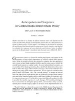
Figure 1 illustrates the problem identified
by Rose (1988) using U.S. data for the ex post 3-
month real interest rate and annualized growth
rate of per capita consumption (nondurable goods
plus services) for 1953:Q1–2007:Q2. The two series
appear to track each other reasonably well for long
periods, such as the 1950s, 1960s, and 1984-2001,
but they also diverge for significant periods, such

as the 1970s, early 1980s, and 2001-05.
The simplest versions of the consumption-
based asset pricing model are based on an endow-
ment economy with a representative household
and constant preferences. The next subsection
discusses the fact that more elaborate theoretical
models allow for some changes in the economy—
for example, changes in fiscal or monetary pol-
icy—to alter the steady-state real interest rate
while leaving steady-state consumption growth
unchanged. That is, they permit a mismatch in
the integration properties of the real interest rate
and consumption growth.
Equilibrium Growth Models and the
Steady-State Real Interest Rate
General equilibrium growth models with a
production technology imply Euler equations
similar to equations (1) and (2) that suggest sources
of a unit root in real interest rates. Specifically, the
Neely and Rapach
FEDERAL RESERVE BANK OF ST
.
LOUIS
REV I EW
NOVEMBER
/
DECEMBER
200 8 611
1955 1960 1965 1970 1975 1980 1985 1990 1995 2000 2005
–6

–4
–2
0
2
4
6
8
10
Ex Post Real Interest Rate
Per Capita Consumption Growth
Percent
Figure 1
U.S. Ex Post Real Interest Rate and Real Per Capita Consumption Growth, 1953:Q1–2007:Q2
NOTE: The figure plots the U.S. ex post 3-month real interest rate and annualized per capita consumption growth. Consumption is
measured as the sum of nondurable goods and services consumption.
Cass (1965) and Koopmans (1965) neoclassical
growth model with a representative profit-
maximizing firm and utility-maximizing house-
hold predicts that the steady-state real interest rate
is a function of time preference, risk aversion,
and the steady-state growth rate of technological
change (Blanchard and Fischer, 1989, Chap. 2;
Barro and Sala-i-Martin, 2003, Chap. 3; Romer,
2006, Chap. 2). In this model the assumption of
constant relative risk aversion utility implies the
following familiar steady-state condition:
(3)
where r* is the steady-state real interest rate,
ζ
= –log͑

β
͒ is the rate of time preference, and z is
the (expected) steady-state growth rate of labor-
augmenting technological change. Equation (3)
implies that a permanent change in the exogenous
rate of time preference, risk aversion, or long-run
growth rate of technology will affect the steady-
state real interest rate.
2
If there is no uncertainty,
the neoclassical growth model implies the follow-
ing steady-state version of the Euler equation
given by (2):
(4)
where [∆log͑c͒]* represents the steady-state
growth rate of c
t
. Substituting the right-hand side
of equation (3) into equation (4) for r*, one finds
that steady-state technology growth determines
steady-state consumption growth: [∆log͑c͒]* = z.
If the rate of time preference (
ζ
), risk aversion
(
α
), and/or steady-state rate of technology growth
(z) change, then (3) requires corresponding
changes in the steady-state real interest rate.
Depending on the size and frequency of such

changes, real interest rates might be very persis -
tent, exhibiting unit root behavior and/or struc-
tural breaks. Of these three factors, a change in
the steady-state growth rate of technology—such
as those that might be associated with the “produc-
tivity slowdown” of the early 1970s and/or the
“New Economy” resurgence of the mid-1990s—is
the only one that will alter both the real interest
rate and consumption growth, producing non-
r z*
=+
ζα
,
−−
()




+=
ζα
∆log ,
c r* *
0
stationary behavior in both variables. Thus, it
cannot explain the mismatch in the integration
properties of the real interest rate and consump-
tion growth identified by Rose (1988).
On the other hand, shocks to the preference
parameters,

ζ
and
α
, will change only the steady-
state real interest rate and not steady-state con-
sumption growth. Therefore, changes in
preferences potentially disconnect the integration
properties of real interest rates and consumption
growth. Researchers generally view preferences
as stable, however, making it unpalatable to
ascribe the persistence mismatch to such changes.
3
In more elaborate models, still other factors
can change the steady-state real interest rate.
For example, permanent changes in government
purchases and their financing can also affect the
steady-state real rate in overlapping generations
models with heterogeneous households
(Samuelson, 1958; Diamond, 1965; Blanchard,
1985; Blanchard and Fischer, 1989, Chap. 3;
Romer, 2006, Chap. 2). Such shocks affect the
steady-state real interest rate without affecting
steady-state consumption growth, so they poten-
tially explain the mismatch in the integration
properties of the real interest rate and consump-
tion growth examined by Rose (1988).
Finally, some monetary growth models allow
for changes in steady-state money growth to affect
the steady-state real interest rate. The seminal
models of Mundell (1963) and Tobin (1965) pre-

dict that an increase in steady-state money growth
lowers the steady-state real interest rate, and more
recent micro-founded monetary models have
similar implications (Weiss, 1980; Espinosa-Vega
and Russell, 1998a,b; Bullard and Russell, 2004;
Reis, 2007; Lioui and Poncet, 2008). Again, this
class of models permits changes in the steady-
state real interest rate without corresponding
changes in consumption growth, potentially
explaining a mismatch in the integration proper-
ties of the real interest rate and consumption
growth.
2
Changes in distortionary tax rates could also affect r* (Blanchard
and Fischer, 1989, pp. 56-59).
Neely and Rapach
612
NOVEMBER
/
DECEMBER
200 8
FEDERAL RESERVE BANK OF ST
.
LOUIS
REV I EW
3
Some researchers appear more willing to allow for changes in
preferences over an extended period. For example, Clark (2007)
argues that a steady decrease in the rate of time preference is respon-
sible for the downward trend in real interest rates in Europe from

the early medieval period to the eve of the Industrial Revolution.
Transitional Dynamics
The previous section discusses factors that
can affect the steady-state real interest rate. Other
shocks can have persistent—but ultimately tran-
sitory—effects on the real rate. For example, in
the neoclassical growth model, a temporary
increase in technology growth or government
purchases leads to a persistently (but not perma-
nently) higher real interest rate (Romer, 2006,
Chap. 2). In addition, monetary shocks can per-
sistently affect the real interest rate via a variety
of frictions, such as “sticky” prices and informa-
tion, adjustment costs, and learning by agents
about policy regimes. Transient technology and
fiscal shocks, as well as monetary shocks, can
also explain differences in the persistence of real
interest rates and consumption growth. For exam-
ple, using a calibrated neoclassical equilibrium
growth model, Baxter and King (1993) show that
a temporary (four-year) increase in government
purchases persistently raises the real interest rate,
although it eventually returns to its initial level.
In contrast, the fiscal shock produces a much less
persistent reaction in consumption growth. As we
will discuss later, evidence of highly persistent
but mean-reverting behavior in real interest rates
supports the empirical relevance of these shocks.
TESTING THE INTEGRATION
PROPERTIES OF REAL INTEREST

RATES
Ex Ante versus Ex Post Real Interest
Rates
The ex ante real interest rate (EARR) is the
nominal interest rate minus the expected inflation
rate, while the ex post real rate (EPRR) is the
nominal rate minus actual inflation. Agents make
economic decisions on the basis of their inflation
expectations over the decision horizon. For exam-
ple, the Euler equations (1) and (2) relate the
expected marginal utility of consumption to the
expected real return. Therefore, the EARR is the
relevant measure for evaluating economic deci-
sions, and we really wish to evaluate the EARR’s
time-series properties, rather than those of the
EPRR.
Unfortunately, the EARR is not directly observ-
able because expected inflation is not directly
observable. An obvious solution is to use some
survey measure of inflation expectations, such
as the Livingston Survey of professional fore-
casters, which has been conducted biannually
since the 1940s (Carlson, 1977). Economists are
often reluctant, however, to accept survey fore-
casts as expectations. For example, Mishkin (1981,
p. 153) expresses “serious doubts as to the quality
of these [survey] data.” Obtaining survey data at
the desired frequency for the desired sample might
create other obstacles to the use of survey data.
Some studies have used survey data, however,

including Crowder and Hoffman (1996) and Sun
and Phillips (2004).
There are at least two alternative approaches
to the problem of unobserved expectations. The
first is to use econometric forecasting methods to
construct inflation forecasts; see, for example,
Mishkin (1981, 1984) and Huizinga and Mishkin
(1986). Unfortunately, econometric forecasting
models do not necessarily include all of the rele-
vant information agents use to form expectations
of inflation, and such models can fail to change
with the structure of the economy. For example,
Stock and Watson (1999, 2003) show that both
real activity and asset prices forecast inflation but
that the predictive relations change over time.
4
A second alternative approach is to use the
actual inflation rate as a proxy for inflation expec-
tations. By definition, the actual inflation rate at
time t (
π
t
) is the sum of the expected inflation rate
and a forecast error term (
ε
t
):
(5)
The literature on real interest rates has long
argued that, if expectations are formed rationally,

E
t–1
π
t
should be an optimal forecast of inflation
(Nelson and Schwert, 1977), and
ε
t
should there-
ππε
t t t t
E
=+
−1
.
Neely and Rapach
FEDERAL RESERVE BANK OF ST
.
LOUIS
REV I EW
NOVEMBER
/
DECEMBER
200 8 613
4
Atkeson and Ohanian (2001) and Stock and Watson (2007) discuss
the econometric challenges in forecasting inflation. One might
also consider using Treasury inflation-protected securities (TIPS)
yields—and/or their foreign counterparts—to measure real inter-
est rates. But these series have a relatively short span of available

data, in that the U.S. securities were first issued in 1997, are only
available at long maturities (5, 10, and 20 years), and do not cor-
rectly measure real rates when there is a significant chance of
deflation.
fore be a white noise process. The EARR can be
expressed (approximately) as
(6)
where i
t
is the nominal interest rate. Solving
equation (5) for E
t
͑
π
t+1
͒ and substituting it into
equation (6), we have
(7)
where r
t
ep
= i
t
–
π
t+1
is the EPRR. Equation (7)
implies that, under rational expectations, the
EPRR and EARR differ only by a white noise com-
ponent, so the EPRR and EARR will share the

same long-run (integration) properties. Actually,
this latter result does not require expectations to
be formed rationally but holds if the expectation
errors (
ε
t+1
) are stationary.
5
Beginning with Rose
(1988), much of the empirical literature tests the
integration properties of the EARR with the EPRR,
after assuming that inflation-expectation errors
are stationary.
Researchers typically evaluate the integration
properties of the EPRR with a decision rule. They
first analyze the individual components of the
EPRR, i
t
and
π
t+1
. If unit root tests indicate that i
t
and
π
t+1
are both I͑0͒, then this implies a station-
ary EPRR, as any linear combination of two I͑0͒
processes is also an I͑0͒ process.
6

If i
t
and
π
t+1
have different orders of integration—for example,
if i
t
~ I͑1͒ and
π
t+1
~ I͑0͒—then the EPRR must
have a unit root, as any linear combination of an
I͑1͒ process and an I͑0͒ process is an I͑1͒ process.
Finally, if unit root tests show that i
t
and
π
t+1
are
both I͑1͒, researchers test for a stationary EPRR
by testing for cointegration between i
t
and
π
t+1
—
that is, testing whether the linear combination
r i E
t

ea
t t t
=−
+
π
1
,
r i
i r
t
ea
t t t
t t t t
ep
t
=− −
()
=− + = +
+ +
+ ++
πε
πε ε
1 1
1 1 1
,
i
t
–[
θ
0

+
θ
1
π
t+1
] is a stationary process—using
one of two approaches.
7
First, many researchers
impose a cointegrating vector of ͑1,–
θ
1
͒′ = ͑1,–1͒′
and apply unit root tests to r
t
ep
= i
t
–
π
t+1
. This
approach typically has more power to reject the
null of no cointegration when the true cointegrat-
ing vector is ͑1,–1͒′. The second approach is to
freely estimate the cointegrating vector between
i
t
and
π

t+1
, as this allows for tax effects (Darby,
1975).
If i
t
,
π
t+1
~ I͑1͒, then a stationary EPRR requires
i
t
and
π
t+1
to be cointegrated with cointegrating
coefficient,
θ
1
= 1, or, allowing for tax effects,
θ
1
= 1/͑1 –
τ
͒, where
τ
is the marginal investor’s
marginal tax rate on nominal interest income.
When allowing for tax effects, researchers view
estimates of
θ

1
in the range of 1.3 to 1.4 as plausi-
ble, as they correspond to a marginal tax rate
around 0.2 to 0.3 (Summers, 1983).
8
It is worth
emphasizing that cointegration between i
t
and
π
t+1
by itself does not imply a stationary real
interest rate:
θ
1
must also equal 1 [or 1/͑1 –
τ
͒],
as other values of
θ
1
imply that the equilibrium
real interest rate varies with inflation.
Although much of the empirical literature
analyzes the EPRR in this manner, it is important
to keep in mind that the EPRR’s time-series prop-
erties can differ from those of the EARR—the
ultimate object of analysis—in two ways. First,
the EPRR’s behavior at short horizons might differ
from that of the EARR. For example, using survey

data and various econometric methods to forecast
inflation, Dotsey, Lantz, and Scholl (2003) study
the behavior of the EARR and EPRR at business-
cycle frequencies and find that their behavior
over the business cycle can differ significantly.
Second, some estimation techniques can gener-
ate different persistence properties between the
EARR and EPRR; see, for example, Evans and
Lewis (1995) and Sun and Phillips (2004).
Early Studies
A collection of early studies on the efficient
market hypothesis and the ability of nominal
5
Peláez (1995) provides evidence that inflation-expectation errors
are stationary. Also note that Andolfatto, Hendry, and Moran (2008)
argue that inflation-expectation errors can appear serially corre-
lated in finite samples, even when expectations are formed ration-
ally, due to short-run learning dynamics about infrequent changes
in the monetary policy regime.
6
The appendix, “Unit Roots and Cointegration Tests,” provides
more information on the mechanics of popular unit root and
cointegration tests.
7
The presence of
θ
0
allows for a constant term in the cointegrating
relationship corresponding to the steady-state real interest rate.
Neely and Rapach

614
NOVEMBER
/
DECEMBER
200 8
FEDERAL RESERVE BANK OF ST
.
LOUIS
REV I EW
8
Data from tax-free municipal bonds would presumably provide a
unitary coefficient. Crowder and Wohar (1999) study the Fisher
effect with tax-free municipal bonds.
interest rates to forecast the inflation rate fore-
shadows the studies that use unit root and coin-
tegration tests. Fama (1975) presents evidence
that the monthly U.S. EARR can be viewed as
constant over 1953-71. Nelson and Schwert (1977),
however, argue that statistical tests of Fama (1975)
have low power and that his data are actually not
very informative about the EARR’s autocorrelation
properties. Hess and Bicksler (1975), Fama (1976),
Carlson (1977), and Garbade and Wachtel (1978)
also challenge Fama’s (1975) finding on statistical
grounds. In addition, subsequent studies show
that Fama’s (1975) result hinges critically on the
particular sample period (Mishkin, 1981, 1984;
Huizinga and Mishkin, 1986; Antoncic, 1986).
Unit Root and Cointegration Tests
The development of unit root and cointegra-

tion analysis, beginning with Dickey and Fuller
(1979), spurred the studies that formally test the
persistence of real interest rates. In his seminal
study, Rose (1988) tests for unit roots in short-term
nominal interest rates and inflation rates using
monthly data for 1947-86 for 18 countries in the
Organisation for Economic Co-operation and
Development (OECD). Rose (1988) finds that aug-
mented Dickey-Fuller (ADF) tests fail to reject
the null hypothesis of a unit root in short-term
nominal interest rates, but they can consistently
reject a unit root in inflation rates based on vari-
ous price indices—consumer price index (CPI),
gross national product (GNP) deflator, implicit
price deflator, and wholesale price index (WPI).
9
As discussed above, the finding that i
t
~ I͑1͒ while
π
t
~ I͑0͒ indicates that the EPRR, i
t
–
π
t+1
, is an I͑1͒
process. Under the assumption that inflation-
expectation errors are stationary, this also implies
that the EARR is an I͑1͒ process. Rose (1988) eas-

ily rejects the unit root null hypothesis for U.S.
consumption growth, which leads him to argue
that an I͑1͒ real interest rate and I͑0͒ consumption
growth rate violates the intertemporal Euler equa-
tion implied by the consumption-based asset pric-
ing model. Beginning with Rose (1988), Table 1
summarizes the methods and conclusions of sur-
veyed papers on the long-run properties of real
interest rates.
A number of subsequent papers also test for
a unit root in real interest rates. Before estimating
structural vector autoregressive (SVAR) models,
King et al. (1991) and Galí (1992) apply ADF unit
root tests to the U.S. nominal 3-month Treasury
bill rate, inflation rate, and EPRR. Using quarterly
data for 1954-88 and the GNP deflator inflation
rate, King et al. (1991) fail to reject the null hypoth-
esis of a unit root in the nominal interest rate,
matching the finding of Rose (1988). Unlike Rose
(1988), however, King et al. cannot reject the unit
root null hypothesis for the inflation rate, which
creates the possibility that the nominal interest
rate and inflation rate are cointegrated. Imposing
a cointegrating vector of ͑1,–1͒′, they fail to reject
the unit root null hypothesis for the EPRR. Using
quarterly data for 1955-87, the CPI inflation rate,
and simulated critical values that account for
potential size distortions due to moving-average
components, Galí (1992) obtains unit root test
results similar to those of King et al. Despite the

failure to reject the null hypothesis that i
t
–
π
t+1
~
I͑1͒, Galí nevertheless assumes that i
t
–
π
t+1
~ I͑0͒
when he estimates his SVAR model, contending
that “the assumption of a unit root in the real
[interest] rate seems rather implausible on a priori
grounds, given its inconsistency with standard
equilibrium growth models” (Galí, 1992, p. 717).
This is in interesting contrast to King et al., who
maintain the assumption that i
t
–
π
t+1
~ I͑1͒ in their
SVAR model. Shapiro and Watson (1988) report
similar unit root findings and, like Galí, still
assume the EPRR is stationary in an SVAR model.
Analyzing a 1953-90 full sample, as well as a
variety of subsamples for the nominal Treasury
bill rate and CPI inflation rate, Mishkin (1992)

argues that monthly U.S. data are largely consis-
tent with a stationary EPRR. With simulated crit-
ical values, as in Galí (1992), Mishkin (1992) finds
that the nominal interest rate and inflation rate
are both I͑1͒ over four sample periods: 1953:01–
1990:12, 1953:01–1979:10, 1979:11–1982:10, and
1982:11–1990:12. He then tests whether the nomi-
nal interest rate and inflation rate are cointegrated
using both the single-equation augmented Engle
and Granger (1987, AEG) test and by prespecify-
Neely and Rapach
FEDERAL RESERVE BANK OF ST
.
LOUIS
REV I EW
NOVEMBER
/
DECEMBER
200 8 615
9
The appendix discusses unit root and cointegration tests.
Neely and Rapach
616
NOVEMBER
/
DECEMBER
200 8
FEDERAL RESERVE BANK OF ST
.
LOUIS

REV I EW
Table 1
Selective Summary of the Empirical Literature on the Long-Run Properties of Real Interest Rates
Study Sample Countries Nominal interest rate and price data
Rose (1988) A: 1892-70, 1901-50 18 OECD countries Long-term corporate bond yield, short-
Q: 1947-86 term commercial paper rate, GNP
M: 1948-86 deflator, CPI, implicit price deflator, WPI
King et al. (1991) Q: 1949-88 U.S. 3-month U.S. Treasury bill rate, implicit
GNP deflator
Galí (1992) Q: 1955-87 U.S. 3-month U.S. Treasury bill rate, CPI

Mishkin (1992) M: 1953-90 U.S. 1- and 3-month Treasury bill rates, CPI


Wallace and Warner Q: 1948-90 U.S. 3-month Treasury bill rate, 10-year
(1993) government bond yield, CPI
Engsted (1995) Q: 1962-93 13 OECD countries Long-term bond yield, CPI

Mishkin and Simon Q: 1962-93 Australia 13-week government bond yield, CPI
(1995)
Crowder and Hoffman Q: 1952-91 U.S. 3-month Treasury bill rate, implicit
(1996) consumption deflator, Livingston
inflation expectations survey, tax data
from various sources
Koustas and Serletis Q: Data begin from 11 OECD countries Various short-term nominal interest rates,
(1999) 1957-72; all data CPI
end in 1995
Bierens (2000) M: 1954-94 U.S. Federal funds rate, CPI

Rapach (2003) A: Data begin in 14 industrialized countries Long-term government bond yield,

1949-65; end in implicit GDP deflator
1994-96
Rapach and Weber Q: 1957-2000 16 OECD countries Long-term government bond yield, CPI
(2004)

Rapach and Wohar Q: 1960-1998 13 OECD countries Long-term government bond yield, CPI
(2004) marginal tax rate data (Padovano and
Galli, 2001)
NOTE: A, Q, and M indicate annual, quarterly, and monthly data frequencies; GNP denotes gross national product.
Neely and Rapach
FEDERAL RESERVE BANK OF ST
.
LOUIS
REV I EW
NOVEMBER
/
DECEMBER
200 8 617


Results on the long-run properties of nominal interest rates, inflation rates, and real interest rates
ADF tests fail to reject a unit root for nominal interest rates but do reject for inflation rates, indicating a unit root
in EPRRs. ADF tests do reject a unit root for consumption growth.

ADF tests fail to reject a unit root for the nominal interest rate, inflation rate, and EPRR.

ADF tests with simulated critical values that adjust for moving-average components fail to reject a unit root in the
nominal interest rate, inflation rate, and EPRR.
ADF tests with simulated critical values that adjust for moving-average components fail to reject a unit root in the
nominal interest rate and inflation rate. AEG tests typically reject the null of no cointegration, indicating a

stationary EPRR.
ADF tests fail to reject a unit root in the long-term nominal interest rate and inflation rate. Johansen (1991)
procedure provides evidence that the variables are cointegrated and that the EPRR is stationary.
ADF tests fail to reject a unit root in nominal interest rates and inflation rates, while cointegration tests present
ambiguous results on the stationarity of the EPRR across countries.
ADF tests fail to reject a unit root in the nominal interest rate and inflation rate. AEG tests typically fail to reject the
null hypothesis of no cointegration, indicating a nonstationary EPRR.
ADF test fails to reject a unit root in the nominal interest rate and inflation rate after accounting for moving-average
components. Johansen (1991) procedure rejects the null of no cointegration and supports a stationary EPRR.


ADF tests usually fail to reject a unit root in nominal interest rates and inflation rates, while KPSS tests typically
reject the null of stationarity, indicating nonstationary nominal interest rates and inflation rates. AEG tests typically
fail to reject the null of no cointegration, indicating a nonstationary EPRR.
New test provides evidence of nonlinear cotrending between the nominal interest rate and inflation rate, indicating
a stationary EPRR. New test, however, cannot distinguish between nonlinear cotrending and linear cointegration.
ADF tests fail to reject a unit root in all nominal interest rates and in 13 of 17 inflation rates. This indicates a
nonstationary EPRR for the four countries with a stationary inflation rate. AEG tests typically fail to reject a unit
root in the EPRR for the 13 countries with a nonstationary inflation rate, indicating a nonstationary EPRR for these
countries.
Ng and Perron (2001) unit root tests typically fail to reject a unit root in nominal interest rates and inflation rates.
Ng and Perron (2001) and Perron and Rodriguez (2001) tests usually fail to reject the null of no cointegration,
indicating a nonstationary EPRR in most countries.
Lower (upper) 95 percent confidence band for the EPRR’s
ρ
is close to 0.90 (above unity) for nearly every country.



Neely and Rapach

618
NOVEMBER
/
DECEMBER
200 8
FEDERAL RESERVE BANK OF ST
.
LOUIS
REV I EW
Table 1, cont’d
Selective Summary of the Empirical Literature on the Long-Run Properties of Real Interest Rates
Study Sample Countries Nominal interest rate and price data
Karanasos, Sekioua, A: 1876-2000 U.S. Long-term government bond yield, CPI
and Zeng (2006)
Lai (1997) Q: 1974-2001 8 industrialized and 1- to 12-month Treasury bill rates, CPI,
8 developing countries Data Resources, Inc. inflation forecasts
Tsay (2000) M: 1953-90 U.S. 1- and 3-month Treasury bill rates, CPI
Sun and Phillips (2004) Q: 1934-94 U.S. 3-month Treasury bill rate, inflation
forecasts from the Survey of
Professional Forecasters, CPI
Pipatchaipoom and M: 1971-2003 U.S. Eurodollar rate, CPI
Smallwood (2008)
Maki (2003) M: 1972-2000 Japan 10-year bond rate, call rate, CPI


Million (2004) M: 1951-99 U.S. 3-month Treasury bill rate, CPI


Christopoulos and Q: 1960-2004 U.S. 3-month Treasury bill rate, CPI
León-Ledesma (2007)





Koustas and Lamarche A: 1960-2004 G-7 countries 3-month government bill rate, CPI
(2008)

Garcia and Perron (1996) Q: 1961-86 U.S. 3-month Treasury bill rate, CPI


Clemente, Montañés, Q: 1980-95 U.S., U.K. Long-term government bond yield, CPI
and Reyes (1998)
Caporale and Grier (2000) Q: 1961-86 U.S. 3-month Treasury bill rate, CPI
Bai and Perron (2003) Q: 1961-86 U.S. 3-month Treasury bill rate, CPI
NOTE: A, Q, and M indicate annual, quarterly, and monthly data frequencies; GNP denotes gross national product.
Neely and Rapach
FEDERAL RESERVE BANK OF ST
.
LOUIS
REV I EW
NOVEMBER
/
DECEMBER
200 8 619


Results on the long-run properties of nominal interest rates, inflation rates, and real interest rates
95 percent confidence interval for the EPRR’s
ρ
is (0.97, 0.99). There is evidence of long-memory, mean-reverting

behavior in the EPRR.
ADF and KPSS tests indicate a unit root in the nominal interest rate, inflation rate, and expected inflation rate.
There is evidence of long-memory, mean-reverting behavior in the EARR and EPRR.
There is evidence of long-memory, mean-reverting behavior in the EPRR.
Bivariate exact Whittle estimator indicates long-memory behavior in the EARR. There is no evidence of a fractional
cointegrating relationship between the nominal interest rate and expected inflation rate.

Exact Whittle estimator provides evidence of long-memory, mean-reverting behavior in the EARR.

Breitung (2002) nonparametric test that allows for nonlinear short-run dynamics provides evidence of cointegration
between the nominal interest rate and inflation rate; cointegrating vector is not estimated, however, so it is not
known if the cointegrating relationship is consistent with a stationary EPRR.
Luukkonen, Saikkonen, and Teräsvirta (1988) test rejects linear short-run dynamics for the adjustment to the long-
run equilibrium EPRR. A smooth transition autoregressive model exhibits asymmetric mean reversion in the EPRR,
depending on the level of the EPRR.
Choi and Saikkonen (2005) test provides evidence of nonlinear cointegration between the nominal interest rate and
inflation rate. Exponential smooth transition regression (ESTR) model fits best over the full sample and the first
subsample (1960-78), while a logistic smooth transition regression (LSTR) model fits best over the second
subsample (1979-2004). Estimated ESTR model for 1960-78 is not consistent with a stationary EPRR for any inflation
rate, and estimated LSTR model for 1979–2004 is consistent with a stationary EPRR only when the inflation rate is
above approximately 3 percent.
ADF and KPSS tests provide evidence of a unit root in the nominal interest rate and inflation rate. Bec, Ben Salem,
and Carassco (2004) nonlinear unit root and Hansen (1996, 1997) linearity tests indicate that the EPRR can be
suitably modeled as a three-regime self-exciting autoregressive (SETAR) process in Canada, France, and Italy.
An estimated autoregressive model with a three-state Markov-switching process for the mean indicates that the
EPRR was in a “moderate”-mean regime for 1961-73, a “low”-mean regime for 1973-80, and a “high”-mean regime
for 1980-86. EPRR is stationary with little persistence within these regimes.
ADF tests that allow for two structural breaks in the mean reject a unit root in the EPRR, indicating that the EPRR is
stationary within regimes defined by structural breaks.
Bai and Perron (1998) methodology provides evidence of multiple structural breaks in the mean EPRR.

Bai and Perron (1998) methodology provides evidence of multiple structural breaks in the mean EPRR.

ing a cointegrating vector and testing for a unit
root in i
t
–
π
t+1
. Mishkin (1992) rejects the null
hypothesis of no cointegration for the 1953:01–
1990:12 and 1953:01–1979:10 periods, but finds
less frequent and weaker rejections for the
1979:11–1982:10 and 1982:11–1990:12 periods.
10
Mishkin and Simon (1995) apply similar tests to
quarterly short-term nominal interest rate and
inflation rate data for Australia. Using a 1962:Q3–
1993:Q4 full sample, as well as 1962:Q3–1979:Q3
and 1979:Q4– 1993:Q4 subsamples, they find
evidence that both the nominal interest rate and
the inflation rate are I͑1͒, agreeing with the results
for U.S. data in Mishkin (1992). There is weaker
evidence that the Australian nominal interest rate
and inflation rate are cointegrated than there is
for U.S. data. Never theless, Mishkin and Simon
(1995) argue that theoretical considerations war-
rant viewing the long-run real interest rate as sta-
tionary in Australia, as “any reasonable model of
the macro economy would surely suggest that
real interest rates have mean-reverting tenden-

cies which make them stationary” (Mishkin and
Simon, 1995, p. 223).
Koustas and Serletis (1999) test for unit roots
and cointegration in short-term nominal interest
rates and CPI inflation rates using quarterly data
for 1957-95 for 11 industrialized countries. They
use ADF unit root tests as well as the KPSS unit
root test of Kwiatkowski et al. (1992), which takes
stationarity as the null hypothesis and nonstation-
arity as the alternative. ADF and KPSS unit root
tests indicate that i
t
~ I͑1͒ and
π
t+1
~ I͑1͒ in most
countries, so a stationary EPRR requires cointegra-
tion between the nominal interest rate and infla-
tion rate. Koustas and Serletis (1999), however,
usually fail to find strong evidence of cointegra-
tion using the AEG test. Overall, their study finds
that the EPRR is nonstationary in many industri-
alized countries. Rapach (2003) obtains similar
results using postwar data for an even larger num-
ber of OECD countries.
In a subtle variation on conventional cointe-
gration analysis, Bierens (2000) allows an individ-
ual time series to have a deterministic component
that is a highly complex function of time—essen-
tially a smooth spline—and a stationary stochastic

component, and he develops nonparametric pro-
cedures to test whether two series share a common
10
Although they use essentially the same econometric procedures
and similar samples, Galí (1992) is unable to reject the unit root
null hypothesis for the EPRR, while Mishkin (1992) does reject
this null hypothesis. This illustrates the sensitivity of EPRR unit
root and cointegration tests to the specific sample. In addition,
the use of short samples, such as the 1979:11–1982:10 sample
period considered by Mishkin (1992), is unlikely to be informative
about the integration properties of the EPRR. To infer long-run
behavior, one needs reasonably long samples.
Neely and Rapach
620
NOVEMBER
/
DECEMBER
200 8
FEDERAL RESERVE BANK OF ST
.
LOUIS
REV I EW
Table 1, cont’d
Selective Summary of the Empirical Literature on the Long-Run Properties of Real Interest Rates
Study Sample Countries Nominal interest rate and price data
Lai (2004) M: 1978-2002 U.S. 1-year Treasury bill rate, inflation
expectations from the University of
Michigan Survey of Consumers, CPI,
federal marginal income tax rates for
four-person families

Rapach and Wohar (2005) Q: 1960-98 13 OECD countries Long-term government bond yield,
CPI, marginal tax rate data (Padovano
and Galli, 2001)
Lai (2008) Q: 1974-2001 8 industrialized and 1- to 12-month Treasury bill rate, deposit
8 developing countries rate, CPI
NOTE: A, Q, and M indicate annual, quarterly, and monthly data frequencies; GNP denotes gross national product.
deterministic component (“nonlinear cotrending”).
Using monthly U.S. data for 1954-94, Bierens
(2000) presents evidence that the federal funds
rate and CPI inflation rate cotrend with a vector
of ͑1,–1͒′, which can be interpreted as evidence
for a stationary real interest rate. Bierens shows,
however, that his tests cannot differentiate
between nonlinear cotrending and linear cointe-
gration in the presence of stochastic trends in
the nominal interest rate and inflation rate. In
essence, the highly complex deterministic com-
ponents for the individual series closely mimic
unit root behavior.
A number of studies use the Johansen (1991)
system–based cointegration procedure to test for
a stationary EPRR. Wallace and Warner (1993)
apply the Johansen (1991) procedure to quarterly
U.S. nominal 3-month Treasury bill rate and CPI
inflation data for a 1948-90 full sample and a
number of subsamples. Their results generally
support the existence of a cointegrating relation-
ship, and their estimates of
θ
1

are typically not
significantly different from unity, in line with a
stationary EPRR. Wallace and Warner (1993) also
argue that the expectations hypothesis implies
that short-term and long-term nominal interest
rates should be cointegrated, and they find evi-
dence that U.S. short and long rates are cointe-
grated with a cointegrating vector of ͑1,–1͒′. In
line with the results for the nominal 3-month
Treasury bill rate, Wallace and Warner find that
the nominal 10-year Treasury bond rate and infla-
tion rate are cointegrated.
With quarterly U.S. data for 1951-91, Crowder
and Hoffman (1996) also use the Johansen (1991)
procedure to test for cointegration between the
3-month Treasury bill rate and implicit consump-
tion deflator inflation rate. As in Wallace and
Warner (1993), they reject the null of no cointe-
gration between the nominal interest rate and
inflation rate. Their estimates of
θ
1
range from
1.22 to 1.34, which are consistent with a station-
ary tax-adjusted EPRR. Crowder and Hoffman
(1996) also use estimates of average marginal tax
rates to directly test for cointegration between
i
t
͑1 –

τ
͒ and
π
t+1
. The Johansen (1991) procedure
supports cointegration and estimates a cointegrat-
ing vector not significantly different from ͑1,–1͒′,
in line with a stationary tax-adjusted EPRR.
Engsted (1995) uses the Johansen (1991) pro-
cedure to test for cointegration between the nomi-
nal long-term government bond yield and CPI
inflation rate in 13 OECD countries using quarterly
data for 1962-93. In broad agreement with the
results of Wallace and Warner (1993) and Crowder
and Hoffman (1996), Engsted (1995) rejects the
Neely and Rapach
FEDERAL RESERVE BANK OF ST
.
LOUIS
REV I EW
NOVEMBER
/
DECEMBER
200 8 621


Results on the long-run properties of nominal interest rates, inflation rates, and real interest rates
ADF tests allowing for a structural break in the mean reject a unit root in the tax-adjusted or unadjusted EARR,
indicating that the EARR is stationary within regimes defined by the structural break.




The Bai and Perron (1998) methodology provides evidence of structural breaks (usually multiple) in the mean EPRR
and mean inflation rate for all 13 countries.

ADF tests allowing for a structural break in the mean reject a unit root in the EPRR for most countries, indicating
that the EPRR is stationary within regimes defined by the structural break.

null hypothesis of no cointegration for almost all
countries. The estimates of
θ
1
vary quite markedly
across countries, however, and the values are
often inconsistent with a stationary EPRR.
Overall, unit root and cointegration tests
present mixed results with respect to the integra-
tion properties of the EPRR. Generally speaking,
single-equation methods provide weaker evidence
of a stationary EPRR, while the Johansen (1991)
system–based approach supports a stationary
EPRR, at least for the United States. Unfortunately,
econometric issues, such as the low power of
unit root tests and size distortions in the presence
of moving-average components, complicate infer-
ence about persistence.
To address these econometric issues, Rapach
and Weber (2004) use unit root and cointegration
tests with improved size and power. Specifically,
they use the Ng and Perron (2001) unit root and

Perron and Rodriguez (2001) cointegration tests.
These tests incorporate aspects of the modified
ADF tests in Elliott, Rothenberg, and Stock (1996)
and Perron and Ng (1996), as well as an adjusted
modified information criterion to select the auto -
regressive (AR) lag order, to develop tests that
avoid size distortions while retaining power.
Rapach and Weber (2004) use quarterly nominal
long-term government bond yield and CPI infla-
tion rate data for 1957-2000 for 16 industrialized
countries. The Ng and Perron (2001) unit root and
Perron and Rodriguez (2001) cointegration tests
provide mixed results, but Rapach and Weber
interpret their results as indicating that the EPRR
is nonstationary in most industrialized countries
over the postwar era.
Updated Unit Root and Cointegration
Test Results for U.S. Data
Tables 2 and 3 illustrate the type of evidence
provided by unit root and cointegration tests for
the U.S. 3-month Treasury bill rate, CPI inflation
rate, and per capita consumption growth rate for
1953:Q1–2007:Q2 (the same data as in Figure 1).
Table 2 reports the ADF statistic, as well as
the MZ
α
statistic from Ng and Perron (2001), which
is designed to have better size and power proper-
ties than the former. Consistent with the literature,
neither test rejects the unit root null hypothesis

for the nominal interest rate. The results are mixed
for the inflation rate: The ADF statistic rejects the
unit root null at the 10 percent level, but the MZ
α
statistic does not reject at conventional signifi-
cance levels. The ADF test result that i
t
~ I͑1͒ while
π
t
~ I͑0͒ means that the EPRR is nonstationary, as
in Rose (1988).
11
The MZ
α
statistic’s failure to
reject the unit root null for either inflation or nomi-
11
A significant moving-average component in the inflation rate could
create size distortions in the ADF statistic that lead us to falsely
reject the unit root null hypothesis for that series. The fact that we
do not reject the unit root null using the MZ
α
statistic—which is
designed to avoid this size distortion—supports this interpretation.
Rapach and Weber (2004), however, do reject the unit root null
for the U.S. inflation rate using the MZ
α
statistic and data through
2000. Inflation rate unit root tests are thus particularly sensitive

to the sample period.
Neely and Rapach
622
NOVEMBER
/
DECEMBER
200 8
FEDERAL RESERVE BANK OF ST
.
LOUIS
REV I EW
Table 2
Unit Root Test Statistics, U.S. data, 1953:Q1–2007:Q2
Variable ADF MZ
α
3-Month Treasury bill rate –2.49 [7] –4.39 [8]
PCE deflator inflation rate –2.72* [4] –5.20 [5]
Ex post real interest rate –3.06** [6] –18.83*** [2]
Per capita consumption growth –4.99*** [4] –42.07*** [2]
NOTE: The ADF and MZ
α
statistics correspond to a one-sided (lower-tail) test of the null hypothesis that the variable has a unit root
against the alternative hypothesis that the variable is stationary. The 10 percent, 5 percent, and 1 percent critical values for the ADF
statistic are –2.58, –2.89, and –3.51; the 10 percent, 5 percent, and 1 percent critical values for the MZ
α
statistic are –5.70, –8.10, and
–13.80. The lag order for the regression model used to compute the test statistic is reported in brackets. *, **, and *** indicate signifi-
cance at the 10 percent, 5 percent, and 1 percent levels. PCE denotes personal consumption expenditures.
nal interest rates argues for cointegration analysis
of those variables to ascertain the EPRR’s integra-

tion properties. When we prespecify a ͑1,–1͒′
cointegrating vector and apply unit root tests to
the EPRR, we reject the unit root null at the 5
percent level using the ADF statistic and at the
1 percent level using the MZ
α
statistic. The U.S.
EPRR appears to be stationary.
To test the null hypothesis of no cointegration
without prespecifying a cointegrating vector,
Table 3 reports the AEG statistic, MZ
α
statistic
from Perron and Rodriguez (2001), and trace sta-
tistic from Johansen (1991). The AEG and trace
statistics reject the null hypothesis of no cointe-
gration at the 10 percent level, and the MZ
α
sta-
tistic rejects the null at the 5 percent level. Table
3 also reports estimates of the cointegrating coef-
ficients,
θ
0
and
θ
1
. Neither the dynamic ordinary
least squares (OLS) nor Johansen (1991) estimates
of

θ
1
are significantly different from unity, indi-
cating a stationary U.S. EPRR. The cointegrating
vector is not estimated precisely enough to
determine whether there is a tax effect.
Tables 2 and 3 provide evidence that the U.S.
EPRR is stationary, although some of the rejections
are marginal. Unit root and cointegration test
results, however, are sensitive to the test proce-
dure and sample period. Studies such as Mishkin
(1992), Wallace and Warner (1993), and Crowder
and Hoffman (1996) find evidence of a stationary
U.S. EPRR, but Koustas and Serletis (1999) and
Rapach and Weber (2004) generally do not. In
contrast, per capita consumption growth is clearly
stationary, as the ADF and MZ
α
statistics in Table 2
both strongly reject the unit root null hypothesis
for this variable. The fact that integration tests
give mixed results for the EPRR’s stationarity and
clear-cut results for consumption growth high-
lights differences in the persistence properties of
the two variables.
Confidence Intervals for the Sum of the
Autoregressive Coefficients
The sum of the AR coefficients,
ρ
, in the AR

representation of i
t
–
π
t+1
equals unity for an I͑1͒
process, while
ρ
< 1 for an I͑0͒ process. It is inher-
ently difficult, however, to distinguish an I͑1͒
process from a highly persistent I͑0͒ process, as
the two types of processes can be observationally
equivalent (Blough, 1992; Faust, 1996).
12
To ana-
Neely and Rapach
FEDERAL RESERVE BANK OF ST
.
LOUIS
REV I EW
NOVEMBER
/
DECEMBER
200 8 623
12
In line with this, Crowder and Hoffman (1996) emphasize that
impulse response analysis indicates that shocks have very persis -
tent effects on the EPRR, although the U.S. EPRR appears to be I͑0͒.
Table 3
Cointegration Test Statistics and Cointegrating Coefficient Estimates, U.S. 3-Month Treasury

Bill Rate and Inflation Rate (1953:Q1–2007:Q2)
Cointegration tests
AEG MZ
α
Trace
–3.07* [6] –17.11** [2] 19.96* [4]
Coefficient estimates
Estimation method
θ
0
θ
1
Dynamic OLS 2.16** (1.01) 0.86*** (0.24)
Johansen (1991) maximum likelihood 0.39 (1.21) 1.44***(0.29)
NOTE: The AEG and MZ
α
statistics correspond to a one-sided (lower-tail) test of the null hypothesis that the 3-month Treasury bill
rate and inflation rate are not cointegrated against the alternative hypothesis that the variables are cointegrated. The 10 percent, 5
percent, and 1 percent critical values for the AEG statistic are –3.07, –3.37, and –3.96; the 10 percent, 5 percent, and 1 percent critical
values for the MZ
α
statistic are –12.80, –15.84, and –22.84. The trace statistic corresponds to a one-sided (upper-tail) test of the null
hypothesis that the 3-month Treasury bill rate and inflation rate are not cointegrated against the alternative hypothesis that the vari-
ables are cointegrated. The 10 percent, 5 percent, and 1 percent critical values for the trace statistic are 18.47, 20.66, and 24.18. The
lag order for the regression model used to compute the test statistic is reported in brackets. *, **, and *** indicate significance at the
10 percent, 5 percent, and 1 percent levels. Standard errors are reported in parentheses.
lyze the theoretical implications of the time-series
properties of the real interest rate, however, we
want to determine a range of values for
ρ

that are
consistent with the data, not only whether
ρ
is
less than or equal to 1. That is, a series with a
ρ
value of 0.95 is highly persistent, even if it does
not contain a unit root per se, and it is much more
persistent than a series with a
ρ
value of, say, 0.4.
To calculate the degree of persistence in the
data—rather than simply trying to determine if
the series is I͑0͒ or I͑1͒—Rapach and Wohar (2004)
compute 95 percent confidence intervals for
ρ
using the Hansen (1999) grid-bootstrap and
Romano and Wolf (2001) subsampling proce-
dures.
13
Using quarterly nominal long-term gov-
ernment bond yield and CPI inflation rate data
for 13 industrialized countries for 1960-68, Rapach
and Wohar (2004) report that the lower bounds
of the 95 percent confidence interval for
ρ
for the
tax-adjusted EPRR are often greater than 0.90,
while the upper bounds are almost all greater
than unity. Similarly, Karanasos, Sekioua, and

Zeng (2006) use a long span of monthly U.S. long-
term government bond yield and CPI inflation
data for 1876-2000 to compute a 95 percent con-
fidence interval for the EPRR’s
ρ
. Their computed
interval, (0.97, 0.99), indicates that the U.S. EPRR
is a highly persistent or near-unit-root process,
even if it does not actually contain a unit root.
With the same U.S. data underlying the
results in Tables 2 and 3, we use the Hansen (1999)
grid-bootstrap and Romano and Wolf (2001) sub-
sampling procedures to compute a 95 percent
confidence interval for
ρ
in the i
t
–
π
t+1
process.
The grid-bootstrap and subsampling confidence
intervals are (0.77, 0.97) and (0.71, 0.97), and the
upper bounds are consistent with a highly persis -
tent process. In contrast, the grid-bootstrap and
subsampling 95 percent confidence intervals or
ρ
for per capita consumption growth are (0.34,
0.70) and (0.37, 0.64). The upper bounds of the
confidence intervals for

ρ
for consumption growth
are less than the lower bounds of the confidence
intervals for
ρ
for the EPRR. This is another way
to characterize the mismatch in the persistence
properties of the EPRR and consumption growth.
Testing for Fractional Integration
Unit root and cointegration tests are designed
to ascertain whether a series is I͑0͒ or I͑1͒, and
the I͑0͒/I͑1͒ distinction implicitly restricts—per-
haps inappropriately—the types of dynamic
processes allowed. In response, some researchers
test for fractional integration (Granger, 1980;
Granger and Joyeux, 1980; Hosking, 1981) in the
EARR and EPRR. A fractionally integrated series
is denoted by I͑d͒, 0 ≤ d ≤ 1. When d = 0, the series
is I͑0͒, and shocks die out at a geometric rate;
when d = 1, the series is I͑1͒, and shocks have
permanent effects or “infinite memory.” An inter-
mediate case occurs when 0 < d < 1: The series is
mean-reverting, as in the I͑0͒ case, but shocks now
die out at a much slower hyperbolic (rather than
geometric) rate. Series in which 0 < d < 1 exhibit
“long memory,” mean-reverting behavior, and
can be substantially more persistent than even a
highly persistent I͑0͒ series.
A number of studies, including Lai (1997),
Tsay (2000), Karanasos, Sekioua, and Zeng (2006),

Sun and Phillips (2004), and Pipatchaipoom and
Smallwood (2008), test for fractional integration
in the U.S. EPRR or EARR. Using U.S. postwar
monthly or quarterly U.S. data, Lai (1997), Tsay
(2000), and Pipatchaipoom and Smallwood (2008)
all present evidence of long-memory, mean-
reverting behavior, as estimates of d for the U.S.
EPRR or EARR typically range from 0.7 to 0.8 and
are significantly above 0 and below 1. Using a
long span of annual U.S. data (1876-2000),
Karanasos, Sekioua, and Zeng (2006) similarly
find evidence of long-memory, mean-reverting
behavior in the EPRR. Sun and Phillips (2004)
develop a new bivariate econometric procedure
that estimates the EARR’s d parameter in the
0.75 to 1.0 range for quarterly postwar U.S. data.
Overall, fractional integration tests indicate
that the U.S. EPRR and EARR do not contain a
13
Andrews and Chen (1994) argue that the sum of the AR coefficients,
ρ
, characterizes the persistence in a series, as it is related to the
cumulative impulse response function and the spectrum at zero
frequency. While conventional asymptotic or bootstrap confidence
intervals do not generate valid confidence intervals for nearly
integrated processes (Basawa et al., 1991), Hansen (1999) and
Romano and Wolf (2001) show that their procedures do generate
confidence intervals for
ρ
with correct first-order asymptotic cov-

erage. Mikusheva (2007) shows, however, that while the Hansen
(1999) grid-bootstrap procedure has correct asymptotical coverage,
the Romano and Wolf (2001) subsampling procedure does not.
Neely and Rapach
624
NOVEMBER
/
DECEMBER
200 8
FEDERAL RESERVE BANK OF ST
.
LOUIS
REV I EW
unit root per se but are mean-reverting and very
persistent. We confirm this by estimating d for the
EPRR using our sample of U.S. data for 1953:Q1–
2007:Q2 with the Shimotsu (2008) semiparametric
two-step feasible exact local Whittle estimator
that allows for an unknown mean in the series.
This estimator refines the Shimotsu and Phillips
(2005) exact local Whittle estimator, and these
authors show that such local Whittle estimators
of d have good properties in Monte Carlo experi-
ments. The estimate of d for the EPRR is 0.71, with
a 95 percent confidence interval of (0.51, 0.90),
so we can reject the hypothesis that d = 0 or d = 1.
This evidence of long-memory, mean-reverting
behavior is consistent with the results from the
literature discussed previously. The estimate of
d for per capita consumption growth is 0.15 with

a standard error of 0.10, so we cannot reject the
hypothesis that d = 0 at conventional significance
levels. This is another manifestation of the dis-
crepancy in persistence between the real interest
rate and consumption growth.
Testing for Threshold Dynamics and
Nonlinear Cointegration
The empirical literature on the real interest
rate typically uses models that assume both the
cointegrating relationship and short-run dynamics
to be linear.
14
Recently, researchers have begun
to relax these linearity assumptions in favor of
nonlinear cointegration or threshold dynamics,
which allow for the cointegrating relationship or
mean reversion to depend on the current values
of the variables. For example, a threshold model
might permit the EPRR to be approximately a
random walk within ±2 percent of some long-run
equilibrium value but to revert strongly to the ±2
percent bands when it wanders outside the
bands.
15
Million (2004) presents evidence that the U.S.
EPRR adjusts in a nonlinear fashion to a long-run
equilibrium level using a logistic smooth transi-
tion autoregressive (LSTAR) model and monthly
U.S. 3-month Treasury bill rate and CPI inflation
rate data for 1951-99. The Lagrange multiplier

test of Luukkonen, Saikkonen, and Teräsvirta
(1988) rejects the null hypothesis of a linear
dynamic adjustment process, and there is evidence
of stronger (weaker) mean reversion in the EPRR
for values of the EPRR below (above) a threshold
level of 2.2 percent. Million (2004) notes that the
weak mean reversion in the upper regime is con-
sistent with the fact that the U.S. real interest rate
was persistently high during much of the 1980s,
and he observes that the Federal Reserve’s prior-
ity on fighting inflation, following the stagflation
of the 1970s, could explain this period of high
real rates. In a vein similar to that of Million,
Koustas and Lamarche (2008) estimate three-
regime self-exciting threshold autoregressive
(SETAR) models to characterize the monetary
policy strategy of “opportunistic disinflation”
(Blinder, 1994; Orphanides and Wilcox, 2002).
Based on the nonlinear unit root test of Bec, Salem,
and Carassco (2004) and Hansen (1996, 1997)
linearity tests, Koustas and Lamarche (2008) con-
clude that the EPRR can be suitably modeled as
a three-regime SETAR process in Canada, France,
and Italy over the postwar period.
16
Christopoulos and León-Ledesma (2007)
examine quarterly U.S. 3-month Treasury bill
rate and CPI inflation rate data for 1960-2004,
permitting the cointegrating relationship itself
to be nonlinear. More precisely, they allow the

cointegrating coefficient (
θ
1
) to vary with the
inflation rate by estimating logistic and smooth
exponential transition regression (LSTR and
ESTR) models. Christopoulos and León-Ledesma
(2007) find significant evidence of nonlinear
cointegration between the nominal interest rate
and inflation rate using the Choi and Saikkonen
(2005) test. Using estimation techniques from
Saikkonen and Choi (2004), the authors conclude
Neely and Rapach
FEDERAL RESERVE BANK OF ST
.
LOUIS
REV I EW
NOVEMBER
/
DECEMBER
200 8 625
14
Studies that allow for fractional integration or structural breaks
also relax some linearity assumptions but in a different way than
those reviewed in this subsection.
15
The purchasing power parity literature often uses these threshold
models (Sarno and Taylor, 2002).
16
Maki (2003) uses the Breitung (2002) nonparametric procedure

that allows for nonlinear adjustment dynamics to test for cointe-
gration between the Japanese nominal interest rate and CPI infla-
tion rate for 1972:01–2000:12. While Maki (2003) finds significant
evidence of cointegration between the nominal interest rate and
inflation rate using the Breitung (2002) test, he does not estimate
the cointegrating vector, so it is not clear that the long-run equi-
librium relationship is consistent with a stationary EPRR.
that the ESTR model fits best over the full sample
(1960:Q1– 2004:Q4) and the first subsample
(1960:Q1–1978:Q1), whereas the LSTR model
fits best over the second subsample (1979:Q1–
2004:Q4). The estimated ESTR model for 1960:Q1–
1978:Q1 is not consistent with a stationary real
EPRR for any inflation rate, and the estimated
LSTR model for 1979:Q1–2004:Q4 is consistent
with a stationary EPRR only when the inflation
rate moves above approximately 3 percent.
In summary, recently developed econometric
procedures provide some evidence of threshold
behavior or nonlinear cointegration in the EPRR
in certain industrialized countries. In some cases,
the threshold models accord well with our intu-
ition about changes in central bank policies.
Although evidence of threshold behavior in real
interest rates is potentially interesting, the models
do not obviate the persistence in real interest rates,
as there are still regimes where the real interest
rate behaves very much like a unit root process.
TESTING FOR REGIME
SWITCHING AND STRUCTURL

BREAKS IN REAL INTEREST RATES
Building on the work of Huizinga and Mishkin
(1986), another strand of the empirical literature
tests for structural breaks in real interest rates.
Accounting for such breaks can substantially
reduce the persistence within the regimes defined
by those breaks (Perron, 1989). Similarly, failing
to account for structural breaks can produce spu-
rious evidence of fractional integration (Jouini
and Nouira, 2006).
Using quarterly U.S. 3-month Treasury bill
rate and CPI inflation rate data for 1961-86, Garcia
and Perron (1996) use Hamilton’s (1989) Markov-
switching approach to test for regime shifts in the
U.S. EPRR. Specifically, they allow the uncondi-
tional mean of an AR(2) process to follow a three-
state Markov process. The three estimated states
correspond to high, middle, and low regimes with
means of approximately 5.5 percent, 1.4 percent,
and –1.8 percent, respectively. The filtered prob-
ability estimates show that the EPRR was likely
in the middle regime from 1961-73, the low regime
from 1973-81, and the high regime from 1981-86.
There is very little persistence within each regime,
as the estimated AR coefficients (
ρ
1
and
ρ
2

in
equation (A1)) are near 0 within regimes. Overall,
Garcia and Perron (1996) argue that the U.S. real
interest rate occasionally experiences sizable
shifts in its mean value, while the real interest
rate is close to constant within the regimes.
Applications of Markov-switching models
typically assume that the model is ergodic, so the
current state will eventually cycle back to any
possible state. Structural breaks have some similar
properties to Markov-switching regimes, but they
are not ergodic—they do not necessarily tend to
revert to previous conditions. Because real interest
rates in Garcia and Perron (1996) exhibit no obvi-
ous tendency to return to previous states, struc-
tural breaks might be considered more appropriate
for modeling real interest rate changes than Markov
switching. Bai and Perron (1998) develop a pow-
erful methodology for testing for multiple struc-
tural breaks in a regression model, and Caporale
and Grier (2000) and Bai and Perron (2003) apply
this methodology to the mean of the U.S. EPRR.
Both studies use quarterly U.S. short-term nominal
interest rate and CPI inflation rate data for 1961-86,
and the estimated break dates are very similar:
1967:Q1, 1972:Q4, and 1980:Q2 in Caporale and
Grier (2000) and 1966:Q4, 1972:Q3, and 1980:Q3
in Bai and Perron (2003). The breaks correspond
to a decrease in the mean EPRR in 1966/1967, a
further decrease in 1972, and a sharp increase in

1980. Caporale and Grier argue that changes in
political regimes—party control of the presidency
and Senate—produce these regime changes.
Rapach and Wohar (2005) extend the work of
Caporale and Grier (2000) and Bai and Perron
(2003) by applying the Bai and Perron (1998)
methodology to the EPRR in 13 industrialized
countries using tax-adjusted nominal long-term
government bond yield and CPI inflation rate data
for 1960-98. They find significant evidence of
structural breaks in the mean of the EPRR in each
of the 13 countries. Rapach and Wohar (2005) also
find that breaks in the mean inflation rate often
coincide with breaks in the mean EPRR for each
country’s data. Furthermore, increases (decreases)
in the mean inflation rate are almost always associ-
ated with decreases (increases) in the mean EPRR.
Neely and Rapach
626
NOVEMBER
/
DECEMBER
200 8
FEDERAL RESERVE BANK OF ST
.
LOUIS
REV I EW
This finding is consistent with the hypothesis
that monetary easing increases inflation and gen-
erates a persistent decline in the real interest rate.

In a comment on Rapach and Wohar (2005),
Caporale and Grier (2005) examine whether politi-
cal regime changes affect the mean U.S. EPRR,
after controlling for the effects of regime changes
in the inflation rate. Caporale and Grier (2005)
find that political regime changes associated with
changes in the party of the president or control
of Congress do not affect the mean EPRR after con-
trolling for inflation. However, the appointments
of Federal Reserve Chairmen Paul Volcker in 1979
and Alan Greenspan in 1987 are associated with
shifts in the mean EPRR even after controlling
for changes in the mean inflation rate.
The previous papers test for structural breaks
under the assumption of stationary within-regime
behavior. In the spirit of Perron (1989), a number
of studies test whether the real interest rate is I͑0͒
after allowing for deterministic shifts in the mean
real rate. Extending the methodology of Perron
and Vogelsang (1992), Clemente, Montañés, and
Reyes (1998) test the unit root null hypothesis for
the U.K. and U.S. EPRR using quarterly long-term
government bond yield and CPI inflation rate data
for 1980-95, allowing for two breaks in the mean
of the EPRR. They find that the EPRR in the United
Kingdom and United States is an I͑0͒ process
around an unconditional mean with two breaks.
Using monthly U.S. 1-year Treasury bill rate data
for 1978-2002 and expected inflation data from
the University of Michigan’s Survey of Consumers,

Lai (2004) finds that the EARR is an I͑0͒ process
with a shift in its unconditional mean in the early
1980s. Lai (2008) extends Lai (2004) by allowing
for a mean shift in quarterly real interest rates for
eight industrialized countries and eight develop-
ing countries and finds widespread support for a
stationary EPRR after allowing for a break in the
unconditional mean.
To further illustrate the prevalence of structural
breaks, we use the Bai and Perron (1998) method-
ology to test for such instability in the uncondi-
tional mean of the U.S. EPRR for 1953:Q1–
2007:Q2.
17
Table 4 reports the results. The proce-
dure finds three changes in the mean that occur
at 1972:Q3, 1980:Q3, and 1989:Q3 and are similar
to those previously identified for the United
States.
18
The breaks are associated with substan-
Neely and Rapach
FEDERAL RESERVE BANK OF ST
.
LOUIS
REV I EW
NOVEMBER
/
DECEMBER
200 8 627

17
We focus on the Bai and Perron (1998) methodology in analyzing
mean real interest rate shifts in updated U.S. data. It would be
interesting in future research to consider regime-switching models
and recently developed structural break tests such as described
by Elliott and Müller (2006).
18
Rapach and Wohar (2005) discuss how the statistics reported in
Table 4 imply that there are three significant breaks in the uncon-
ditional mean.
Table 4
Bai and Perron (1988) Test Statistics and Estimation Results for the U.S. ex post Real Interest
Rate (1953:Q1–2007:Q2)
Estimated ex post
Test statistic Regime real interest rate mean
UD
max
14.84*** 1953:Q1–1972:Q3 [1969:Q2, 1973:Q4] 1.22*** (0.17)
WD
max
(5%) 27.06** 1972:Q4–1980:Q3 [1979:Q1, 1980:Q4] –0.55 (0.38)
F(1|0) 12.92*** 1980:Q4–1989:Q3 [1984:Q3–1994:Q2] 4.58*** (0.71)
F(2|1) 17.89*** 1989:Q4–2007:Q2 1.82*** (0.52)
F(3|2) 17.89***
F(4|3) 10.37*
F(5|4) 10.37
NOTE: *, **, and *** indicate significance at the 10 percent, 5 percent, and 1 percent levels. The bracketed dates in the Regime column
denote a 90 percent confidence interval for the end of the regime. Numbers in parentheses in the last column denote standard errors
for the estimated mean.
tial changes in the average annualized real inter-

est rate in the different regimes. The average real
rate is 1.22 percent for 1953:Q1–1972:Q3, is not
significantly different from zero for 1972:Q4–
1980:Q3, increases to 4.58 percent for 1980:Q4–
1989:Q3, and falls to 1.82 percent for 1989:Q4–
2007:Q2. Figure 2 depicts the EPRR and the mean
for each of the four regimes defined by the three
breaks.
19
In contrast to this evidence for breaks
in the real rate, the Bai and Perron (1998) method-
ology fails to discover significant evidence of
structural breaks in the mean of per capita con-
sumption growth. (We omit complete results for
brevity.)
In interpreting structural break results, we
emphasize that such breaks only reduce within-
regime or local persistence in real interest rates.
The existence of breaks still implies a high degree
of global persistence, and the breaks themselves
require an economic explanation.
THEORETICAL IMPLICATIONS
AND A MONETARY EXPLANATION
OF PERSISTENCE
This section considers what types of shocks
are most likely to produce the persistence in the
U.S. real interest rate. The empirical literature
devotes relatively little attention to this important
issue. We argue that monetary shocks likely drive
the persistence in the U.S. real interest rate.

19
The test results of Bai and Perron (1998) for structural breaks in the
mean EPRR do not appear sensitive to whether the tax-adjusted or
tax-unadjusted EPRR is used (Rapach and Wohar, 2005). Neither
do estimates of the sum of the AR coefficients nor tests for fractional
integration hinge critically on whether the EPRR is tax adjusted.
Neely and Rapach
628
NOVEMBER
/
DECEMBER
200 8
FEDERAL RESERVE BANK OF ST
.
LOUIS
REV I EW
1955 1960 1965 1970 1975 1980 1985 1990 1995 2000 2005
–6
–4
–2
0
2
4
6
8
10
Ex Post Real Interest Rate
Regime-Specific Means
Percent
Figure 2

U.S. Ex Post Real Interest Rate and Regime-Specific Means, 1953:Q1–2007:Q2
NOTE: The figure plots the U.S. ex post real interest rate and means for the regimes defined by the structural breaks estimated using
the Bai and Perron (1998) methodology.
Before discussing potential sources of real
interest rate persistence, we briefly make the
case that the U.S. real interest rate is ultimately
mean-reverting. As we emphasize, unit root and
cointegration tests have difficulty distinguishing
unit root processes from persistent but stationary
alternatives. Nevertheless, unit root and cointe-
gration tests with good size and power, applied to
updated data, provide evidence that the U.S. real
interest rate is an I͑0͒—and thus mean-reverting—
process (see Table 2).
20
Tests for fractional integra-
tion nest the I͑0͒/I͑1͒ alternatives, and they concur
that the U.S. real interest rate is a mean-reverting
process. Using an updated sample, we confirm the
findings of Lai (1997), Tsay (2000), Pipatchaipoom
and Smallwood (2008), and Karanasos, Sekioua,
and Zeng (2006) that demonstrate long-memory,
mean-reverting behavior in the U.S. real interest
rate. Our updated sample also provides evidence
of structural breaks in the U.S. real interest rate.
Curiously, the regime-specific mean breaks for the
EPRR largely cancel each other in the long run
(see Table 4): The estimated mean real rate in 2007
is close to that estimated for 1953.
21

We specu-
late that although structural breaks appear to
describe the data better than a constant, linear
data generating process, these breaks appear to
exhibit a certain type of mean-reverting behavior.
With sufficient data—much more than we have
now—one could presumably model this mean-
reversion in regimes.
These facts lead us to tentatively claim that
the U.S. real interest rate is best viewed as a very
persistent but ultimately mean-reverting process.
We emphasize the tentative nature of this claim,
and we consider careful econometric testing of
this proposition to be an important area for future
research. Even if real interest rates ultimately
mean-revert, they are clearly very persistent.
Recall the underlying motivation for learning
about real interest rate persistence: In a simple
endowment economy, the real interest rate should
have the same persistence properties as consump-
tion growth. In fact, however, real rates are much
more persistent than consumption growth. Perma -
nent technology growth shocks can create a non-
stationary real rate but affect consumption growth
in the same way, so they cannot account for the
mismatch in persistence. More complex equilib-
rium growth models potentially explain this per-
sistence mismatch through changing fiscal and
monetary policy, as well as transient technology
growth shocks. We consider fiscal, monetary, and

transient technology shocks as potential causes
of persistent fluctuations in the U.S. real interest
rate.
Figures 1 and 2 reveal two episodes of pro-
nounced and prolonged changes in the U.S. EPRR:
the protracted decrease in the EPRR in the 1970s
and subsequent sharp increase in the 1980s. Fiscal
shocks appear to be an unlikely explanation for
the large decline in real rates from 1972-79. The
U.S. did not undertake the sort of contractionary
fiscal policy that would be necessary for such a
fall in real rates.
22
In fact, fiscal policy in the 1970s
largely tended toward modest deficits. Given the
substantial budget deficits beginning in 1981,
expansionary fiscal shocks are a more plausible
candidate for the increase in real rates at this time.
Monetary shocks appear to fit well with the
overall pattern in the real interest rate, including
the multiyear decline in the real rate during the
1970s, the very sharp 1980 increase, and subse-
quent gradual decline during the “Great
Disinflation.” One interpretation of the “Great
Inflation” that began in the late 1960s and lasted
throughout the 1970s is that the Federal Reserve
pursued an expansionary monetary policy—either
inadvertently or to reduce the unemployment rate
to unsustainable levels—and this persistently
reduced the real interest rate (Delong, 1997; Barsky

and Kilian, 2002; Meltzer, 2005; Romer, 2005).
After Paul Volcker’s appointment as Chairman,
the Federal Reserve sharply raised short-term
nominal interest rates to reduce inflation from
its early 1980 peak of nearly 12 percent, and this
Neely and Rapach
FEDERAL RESERVE BANK OF ST
.
LOUIS
REV I EW
NOVEMBER
/
DECEMBER
200 8 629
20
Recall, however, that unit root and cointegration tests are sensitive
to the particular sample used.
21
One might wonder if the observed mean-reversion in structural
breaks contradicts our contention that the breaks should not be
modeled as a Markov process because they are not ergodic. We do
not think, however, that observing one state twice and two states
once provides sufficient information for a Markov process.
22
The recent analyses by Romer and Romer (2008) and Ramey (2008)
indicate that the U.S. economy did not experience sizable con-
tractionary fiscal policy shocks during the 1970s.
produced a sharp and prolonged increase in the
real interest rate. The structural breaks manifest
these pronounced swings: The mean EPRR falls

from 1.22 percent in 1972:Q3 to essentially zero
and then rises to 4.58 percent beginning in
1980:Q4 (see Table 4). Furthermore, Rapach and
Wohar (2005) report evidence of breaks in the
mean U.S. inflation rate in 1973:Q1 and 1982:Q1
that increase and decrease the average inflation
rate. The timing and direction of the breaks are
consistent with a monetary explanation that also
accounts for the mismatch in persistence between
the real interest rate and consumption growth. In
each case, negative (positive) breaks to the real
rate of interest coincide with positive (negative)
breaks in the mean rate of inflation. The data are
in line with the hypothesis that central banks
change monetary policy and inflation through
persistent effects on the real rate of interest.
Turning to technology shocks, the paucity of
independent data on technology shocks makes it
difficult to correlate such changes with real inter-
est rates. In addition, researchers have tradition-
ally viewed technology growth as reasonably
stable. One might think that other sorts of supply
shocks, such as oil price increases, might influence
the real rate, and they surely do to some degree;
Barro and Sala-i-Martin (1990) and Caporale and
Grier (2000), for example, consider this possibil-
ity. It is unlikely, however, that oil price shocks
alone can account for the pronounced swings in
the U.S. real interest rate: Why would rising oil
prices in 1973 reduce the real interest rates but

rising oil prices in 1979 dramatically raise the
real rate?
23
While we interpret the timing of major swings
in the U.S. real rate to strongly suggest a mone-
tary explanation, we ultimately need to estimate
23
Furthermore, Barsky and Kilian (2002) argue that the timing of
increases in U.S. inflation in the early 1970s is more consistent
with a monetary rather than an oil price shock explanation.
Neely and Rapach
630
NOVEMBER
/
DECEMBER
200 8
FEDERAL RESERVE BANK OF ST
.
LOUIS
REV I EW
1970 1975 1980 1985 1990 1995
–1.5
–1
–0.5
0
0.5
1
1.5
Figure 3
Romer and Romer (2004) Measure of Monetary Policy Shocks, 1969:Q1–1996:Q4

NOTE: A positive (negative) value corresponds to a contractionary (expansionary) monetary policy shock.
structural models to analyze the relative impor-
tance of various shocks. Galí (1992) is one of the
few studies providing evidence on the economic
sources of real interest rate persistence. His SVAR
model finds that an expansionary money supply
shock leads to a very persistent decline in the real
interest rate, and money supply shocks account
for nearly 90 percent of the variance in the real
rate at the one-quarter horizon and still account
for around 60 percent of the variance at the 20-
quarter horizon. Galí’s (1992) evidence is consis-
tent with our monetary explanation of real interest
rate persistence.
24
We present tentative additional evidence in
support of a monetary explanation of real interest
rate persistence based on the new measure of
monetary shocks developed by Romer and
Romer (2004). They cull through quantitative
and narrative Federal Reserve records to compute
a monetary policy shock series for 1969-96 that
is independent of systematic responses to antici-
pated economic conditions. Figure 3 plots the
Romer and Romer (2004) monetary policy shocks
series, where expansionary (i.e., negative) shocks
in the late 1960s and early 1970s and large con-
tractionary (i.e., positive) shocks in the late 1970s
and early 1980s appear to match well with the
decline in the U.S. real interest rate in the 1970s

and subsequent sharp increase around 1980.
Romer and Romer (2004) estimate autoregres-
sive distributed lag (ARDL) models to examine
the effects of a monetary policy shock on real
output and the price level. They find that a con-
tractionary shock creates persistent and sizable
Neely and Rapach
FEDERAL RESERVE BANK OF ST
.
LOUIS
REV I EW
NOVEMBER
/
DECEMBER
200 8 631
24
King and Watson (1997) and Rapach (2003) use SVAR frameworks
to estimate the long-run effects of exogenous changes in inflation
on the real interest rate. Both studies find evidence that an exoge-
nous increase in the steady-state inflation rate decreases the
steady-state real interest rate.
0 2 4 6 8 10 12 14 16 18 20
–1
0
1
2
3
4
Quarters After Shock
Percent

Figure 4
U.S. Ex Post Real Interest Rate Response to a Contractionary Romer and Romer (2004)
Monetary Policy Shock
NOTE: The response is based on an autoregressive distributed lag model estimated for 1969:Q1–1996:Q4. Dashed lines delineate
two-standard-error bands. The response is to a shock of size 0.5.
declines in both real output and the price level.
In similar fashion, we estimate an ARDL model via
OLS to measure the effects of a monetary policy
shock on the real interest rate. The ARDL model
takes the form,
(8)
where r
t
ep
is the EPRR and S
t
is the Romer and
Romer measure of monetary policy shocks.
Figure 4 illustrates the response of the EPRR
to a monetary policy shock of size 0.5, which is
comparable to some of the contractionary shocks
experienced in the late 1970s and early 1980s
(see Figure 3). Romer and Romer’s (2004) Monte
Carlo methods provide the two-standard-error
bands. A contractionary monetary policy shock
produces a statistically and economically signif-
icant increase in the U.S. EPRR, which remains
statistically significant after approximately two
years. Note that the response in Figure 4 is nearly
identical to the response of r

t
ep
to a shock to S
t
obtained from a bivariate VAR(8) model that orders
S
t
first in a Cholesky decomposition. Together,
Figures 3 and 4 show that expansionary (contrac-
tionary) monetary policy shocks can account for
the pronounced and prolonged decrease (increase)
in the U.S. real interest rate in the 1970s (early
1980s). We emphasize that this evidence is sug-
gestive. Of course, structural identification is a
thorny issue, and more research is needed to
determine the veracity of the monetary explana-
tion for U.S. real interest rate persistence.
CONCLUSION
Rose’s (1988) seminal study spurred a sizable
empirical literature that examines the time-series
properties of real interest rates. Our survey details
the evidence that real interest rates are highly
persistent. This persistence manifests itself in
the following ways:
• Under the assumption of a constant data
generating process, many studies indicate
that real interest rates contain a unit root.
While econometric problems prevent a
r a a r b S u
t

ep
j t j
ep
j t j
j
t
j
=+ + +
−−
==
∑∑
0
0
8
1
8
,
dispositive resolution of this question, real
interest rates display behavior that is very
persistent, close to a unit root.
• Estimated 95 percent confidence intervals
for the sum of the AR coefficients from the
literature have upper bounds that are greater
than or very near unity.
• Real interest rates appear to display long-
memory behavior; shocks are very long-
lived, but the real interest rate is estimated
to be ultimately mean-reverting.
• Studies allowing for nonlinear dynamics
in real interest rates identify regimes where

the real interest behaves like a unit root
process.
• Structural breaks in unconditional means
characterize real interest rates. Although
the breaks reduce within-regime persis -
tence, the real interest rate remains highly
persistent because the regimes have differ-
ent means.
Although researchers have used a variety of
econometric models to analyze the time-series
properties of real interest rates, relatively little
work has been done to discriminate among these
sundry models. Model selection could tell us, for
example, whether we should think of persistent
changes in real interest rates in terms of changes
in the steady-state real rate—which are consistent
with unit root behavior—or long-lived shocks
that eventually decay to a stable steady-state real
rate—which are consistent with mean-reverting
behavior. While model selection raises challeng-
ing econometric (and philosophical) issues, out-
of-sample forecasting exercises and analysis of
posterior model probabilities in a Bayesian con-
text might identify the best way to model real
interest rate persistence.
Finally, structural analysis is necessary to
identify the sources of the persistence in real
interest rates. Theoretical models suggest that a
variety of shocks can induce real rate persistence,
including preference, technology growth, fiscal,

and monetary shocks. We suggest a tentative
monetary explanation of U.S. real interest rate
persistence based on timing, lack of persistence
in consumption growth, and large and persistent
Neely and Rapach
632
NOVEMBER
/
DECEMBER
200 8
FEDERAL RESERVE BANK OF ST
.
LOUIS
REV I EW
real interest rate responses to a Romer and Romer
(2004) monetary policy shock. The literature
would greatly benefit from further analysis of the
relative importance of different types of shocks
in explaining real interest rate persistence.
REFERENCES
Andolfatto, David; Hendry, Scott and Moran, Kevin.
“Are Inflation Expectations Rational?” Journal of
Monetary Economics, March 2008, 55(2), pp. 406-22.
Andrews, Donald W.K. and Chen, Hong-Yuan.
“Approximately Median-Unbiased Estimation of
Autoregressive Models.” Journal of Business and
Economic Statistics, April 1994, 12(2), pp. 187-204.
Antoncic, Madelyn. “High and Volatile Real Interest
Rates: Where Does the Fed Fit In?” Journal of
Money, Credit, and Banking, February 1986, 18(1),

pp. 18-27.
Atkeson, Andrew and Ohanian, Lee E. “Are Phillips
Curves Useful for Forecasting Inflation?” Federal
Reserve Bank of Minneapolis Quarterly Review,
Winter 2001, 25(1), pp. 2-11.
Bai, Jushan and Perron, Pierre. “Estimating and
Testing Linear Models with Multiple Structural
Changes.” Econometrica, 1998, 66(1), pp. 47-78.
Bai, Jushan and Perron, Pierre. “Computation and
Analysis of Multiple Structural Change Models.”
Journal of Applied Econometrics, January 2003,
18(1), pp. 1-22.
Barro, Robert J. and Sala-i-Martin, Xavier. “World
Real Interest Rates,” in Olivier J. Blanchard and
Stanley Fischer, eds., NBER Macroeconomics
Annual 1990. Cambridge, MA: MIT Press, 1990,
pp. 15-61.
Barro, Robert J. and Sala-i-Martin, Xavier. Economic
Growth. Second Edition. Cambridge, MA: MIT Press,
2003.
Barsky, Robert B. and Kilian, Lutz. “Do We Really
Know that Oil Caused the Great Stagflation? A
Monetary Alternative,” in Ben S. Bernanke and
Kenneth S. Rogoff, eds., NBER Macroeconomics
Annual 2001. Cambridge, MA: MIT Press, 2002,
pp. 137-83.
Basawa, I.V.; Mallik, A.K.; McCormick, W.P.; Reeves,
J.H. and Taylor, R.L. “Bootstrapping Unstable First-
Order Autoregressive Processes.” Annals of
Statistics, June 1991, 19(2), pp. 1098-101.

Baxter, Marianne and King, Robert G. “Fiscal Policy
in General Equilibrium.” American Economic
Review, June 1993, 83(3), pp. 315-34.
Bec, Frédérique; Ben Salem, Mélika and Carassco,
Marine. “Tests for Unit-Root versus Threshold
Specification with an Application to the Purchasing
Power Parity Relationship.” Journal of Business
and Economic Statistics, October 2004, 22(4),
pp. 382-95.
Bierens, Herman J. “Nonparametric Nonlinear
Cotrending Analysis, with an Application to
Interest and Inflation in the United States.” Journal
of Business and Economic Statistics, July 2000,
18(3), pp. 323-37.
Blanchard, Olivier J. “Debt, Deficits, and Finite
Horizons.” Journal of Political Economy, April
1985, 93(2), pp. 223-47.
Blanchard, Olivier J. and Fischer, Stanley. Lectures
on Macroeconomics. Cambridge, MA: MIT Press,
1989.
Blinder, Alan S. “Opening Statement of Alan S.
Blinder at Confirmation Hearing Before the U.S.
Senate Committee on Banking, Housing, and Urban
Affairs.” Unpublished manuscript, Board of
Governors of the Federal Reserve System, May 1994.
Blough, Stephen R. “The Relationship Between
Power and Level for Generic Unit Root Tests in
Finite Samples.” Journal of Applied Econometrics,
July-September 1992, 7(3), pp. 295-308.
Breeden, Douglas T. “An Intertemporal Asset Pricing

Model with Stochastic Consumption and Investment
Opportunities.” Journal of Financial Economics,
September 1979, 7(3), pp. 265-96.
Neely and Rapach
FEDERAL RESERVE BANK OF ST
.
LOUIS
REV I EW
NOVEMBER
/
DECEMBER
200 8 633