Linear stability analysis of a hot plasma in a solid torus
Bạn đang xem bản rút gọn của tài liệu. Xem và tải ngay bản đầy đủ của tài liệu tại đây (513.1 KB, 51 trang )
Linear Stability Analysis of a Hot Plasma in a Solid Torus∗
Toan T. Nguyen†
Walter A. Strauss‡
August 7, 2013
arXiv:1308.1177v1 [math.AP] 6 Aug 2013
Abstract
This paper is a first step toward understanding the effect of toroidal geometry on the rigorous
stability theory of plasmas. We consider a collisionless plasma inside a torus, modeled by the
relativistic Vlasov-Maxwell system. The surface of the torus is perfectly conducting and it
reflects the particles specularly. We provide sharp criteria for the stability of equilibria under
the assumption that the particle distributions and the electromagnetic fields depend only on the
cross-sectional variables of the torus.
Contents
1 Introduction
1.1 Toroidal symmetry .
1.2 Equilibria . . . . . .
1.3 Spaces and operators
1.4 Main results . . . . .
2 The
2.1
2.2
2.3
2.4
2.5
2.6
.
.
.
.
.
.
.
.
.
.
.
.
.
.
.
.
.
.
.
.
.
.
.
.
.
.
.
.
.
.
.
.
.
.
.
.
.
.
.
.
symmetric system
The equations in toroidal coordinates .
Boundary conditions . . . . . . . . . .
Linearization . . . . . . . . . . . . . .
The Vlasov operators . . . . . . . . . .
Growing modes . . . . . . . . . . . . .
Properties of L0 . . . . . . . . . . . .
3 Linear stability
3.1 Invariants . . . . .
3.2 Growing modes are
3.3 Minimization . . .
3.4 Proof of stability .
. . .
pure
. . .
. . .
.
.
.
.
.
.
.
.
.
.
.
.
.
.
.
.
.
.
.
.
.
.
.
.
.
.
.
.
.
.
.
.
.
.
.
.
.
.
.
.
.
.
.
.
.
.
.
.
.
.
.
.
.
.
.
.
.
.
.
.
.
.
.
.
.
.
.
.
.
.
.
.
.
.
.
.
.
.
.
.
.
.
.
.
.
.
.
.
.
.
.
.
.
.
.
.
.
.
.
.
.
.
.
.
.
.
.
.
.
.
.
.
.
.
.
.
.
.
.
.
.
.
.
.
.
.
.
.
.
.
.
.
.
.
.
.
2
4
5
6
8
.
.
.
.
.
.
.
.
.
.
.
.
.
.
.
.
.
.
.
.
.
.
.
.
.
.
.
.
.
.
.
.
.
.
.
.
.
.
.
.
.
.
.
.
.
.
.
.
.
.
.
.
.
.
.
.
.
.
.
.
.
.
.
.
.
.
.
.
.
.
.
.
.
.
.
.
.
.
.
.
.
.
.
.
.
.
.
.
.
.
.
.
.
.
.
.
.
.
.
.
.
.
.
.
.
.
.
.
.
.
.
.
.
.
.
.
.
.
.
.
.
.
.
.
.
.
.
.
.
.
.
.
.
.
.
.
.
.
.
.
.
.
.
.
.
.
.
.
.
.
.
.
.
.
.
.
9
9
10
11
12
13
14
.
.
.
.
.
.
.
.
.
.
.
.
.
.
.
.
.
.
.
.
.
.
.
.
.
.
.
.
.
.
.
.
.
.
.
.
.
.
.
.
.
.
.
.
.
.
.
.
.
.
.
.
.
.
.
.
.
.
.
.
.
.
.
.
.
.
.
.
.
.
.
.
.
.
.
.
.
.
.
.
.
.
.
.
.
.
.
.
.
.
.
.
.
.
.
.
.
.
.
.
.
.
.
.
14
14
16
18
21
†
Department of Mathematics, Pennsylvania State University, University Park, PA 16802, USA. Email:
‡
Department of Mathematics and Lefschetz Center for Dynamical Systems, Brown University, Providence, RI
02912, USA. Email:
∗
Research of the authors was supported in part by the NSF under grants DMS-1108821 and DMS-1007960.
1
4 Linear instability
4.1 Particle trajectories . . . . . . . . . . .
4.2 Representation of the particle densities
4.3 Operators . . . . . . . . . . . . . . . .
4.4 Reduced matrix equation . . . . . . .
4.5 Solution of the matrix equation . . . .
4.6 Existence of a growing mode . . . . .
.
.
.
.
.
.
.
.
.
.
.
.
.
.
.
.
.
.
.
.
.
.
.
.
.
.
.
.
.
.
.
.
.
.
.
.
.
.
.
.
.
.
.
.
.
.
.
.
.
.
.
.
.
.
.
.
.
.
.
.
.
.
.
.
.
.
.
.
.
.
.
.
.
.
.
.
.
.
.
.
.
.
.
.
.
.
.
.
.
.
.
.
.
.
.
.
.
.
.
.
.
.
.
.
.
.
.
.
.
.
.
.
.
.
.
.
.
.
.
.
.
.
.
.
.
.
.
.
.
.
.
.
.
.
.
.
.
.
.
.
.
.
.
.
.
.
.
.
.
.
.
.
.
.
.
.
22
23
24
24
30
34
38
5 Examples
39
5.1 Stable equilibria . . . . . . . . . . . . . . . . . . . . . . . . . . . . . . . . . . . . . . 39
5.2 Unstable equilibria . . . . . . . . . . . . . . . . . . . . . . . . . . . . . . . . . . . . . 40
A Toroidal coordinates
45
B Scalar operators
46
C Equilibria
47
D Particle trajectories
48
1
Introduction
Stability analysis is a central issue in the theory of plasmas (e.g., [22], [25]). In the search for
practical fusion energy, the tokamak has been the central focus of research for many years. The
classical tokamak has two features, the toroidal geometry and a mechanism (magnetic field, laser
beams) to confine the plasma. Here we concentrate on the effect of the toroidal geometry on the
stability analysis of equilibria.
When a plasma is very hot (or of low density), electromagnetic forces have a much faster
effect on the particles than the collisions, so the collisions can be ignored as compared with the
electromagnetic forces. So such a plasma is modeled by the relativistic Vlasov-Maxwell system
(RVM)
∂t f + + vˆ · ∇x f + + (E + vˆ × B) · ∇v f + = 0,
(1.1)
∂t f − + vˆ · ∇x f − − (E + vˆ × B) · ∇v f − = 0,
∇x · E = ρ,
∂t E − ∇x × B = −j,
ρ=
R3
(f + − f − ) dv,
∇x · B = 0,
(1.2)
∂t B + ∇x × E = 0,
(1.3)
j=
R3
vˆ(f + − f − ) dv.
Here f ± (t, x, v) ≥ 0 denotes the density distribution of ions and electrons, respectively, x ∈ Ω ⊂ R3
is the particle position, Ω is the region occupied by the plasma, v ∈ R3 is the particle momentum,
v = 1 + |v|2 is the particle energy, vˆ = v/ v the particle velocity, ρ the charge density, j the
current density, E the electric field, B the magnetic field and ±(E + vˆ × B) the electromagnetic
2
force. For simplicity all the constants have been set equal to 1; however, our results do not depend
on this normalization.
The Vlasov-Maxwell system is assumed to be valid inside a solid torus (see Figure 1), which we
take for simplicity to be
Ω = x = (x1 , x2 , x3 ) ∈ R3 :
x21 + x22
a−
2
+ x23 < 1 .
The specular condition at the boundary is
f ± (t, x, v) = f ± (t, x, v − 2(v · n(x))n(x)),
n(x) · v < 0,
x ∈ ∂Ω,
(1.4)
where n(x) denotes the outward normal vector of ∂Ω at x. The perfect conductor boundary
condition is
E(t, x) × n(x) = 0,
B(t, x) · n(x) = 0,
x ∈ ∂Ω.
(1.5)
A fundamental property of RVM with these boundary conditions is that the total energy
E(t) =
v (f + + f − ) dvdx +
Ω
R3
1
2
Ω
|E|2 + |B|2 dx
is conserved in time. In fact, the system admits infinitely many equilibria. The main focus of the
present paper is to investigate the stability properties of the equilibria.
Our analysis is closely related to the spectral analysis approach in [18, 20] which tackled the
stability problem in domains without any spatial boundaries. A first such analysis in a domain
with boundary appears in [21], which treated a 2D plasma inside a circle. Roughly speaking,
these papers provided a sharp stability criterion L0 ≥ 0, where L0 is a certain nonlocal self-adjoint
operator that acts merely on scalar functions depending only on the spatial variables. This positivity
condition was verified explicitly for a number of interesting examples. It may also be amenable
to numerical verification. Now, in the presence of a boundary, every integration by parts brings
in boundary terms and the curvature of the torus plays an important role. We consider a certain
class of equilibria and make some symmetry assumptions, which are spelled out in the next two
subsections. Our main theorems are stated in the third subsection.
Of course, this paper is a rather small step in the direction of mathematically understanding
a confined plasma. Most stability studies ([5], [6], [7], [16], [26]) are based on macroscopic MHD
or other approximate fluids-like models. But because many plasma instability phenomena have
an essentially microscopic nature, kinetic models like Vlasov-Maxwell are required. The VlasovMaxwell system is a rather accurate description of a plasma when collisions are negligible, as occurs
for instance in a hot plasma. The methods of this paper should also shed light on approximate
models like MHD.
Instabilities in Vlasov plasmas reflect the collective behavior of all the particles. Therefore the
instability problem is highly nonlocal and is difficult to study analytically and numerically. In most
of the physics literature on stability (e.g., [25]), only a homogeneous equilibrium with vanishing
electromagnetic fields is treated, in which case there is a dispersion relation that is rather easy to
study analytically. The classical result of this type is Penrose’s sharp linear instability criterion
3
([23]) for a homogeneous equilibrium of the Vlasov-Poisson system. Some further papers on the
stability problem, including nonlinear stability, for general inhomogeneous equilibria of the VlasovPoisson system can be found in [24], [11], [12], [13], [3] and [17]. Among these papers the closest
analogue to our work in a domain with specular boundary conditions is [3].
However, as soon as magnetic effects are included and even for a homogeneous equilibrium, the
stability problem becomes quite complicated, as for the Bernstein modes in a constant magnetic
field [25]. The stability problem for inhomogeneous (spatially-dependent) equilibria with nonzero
electromagnetic fields is yet more complicated and so far there are relatively few rigorous results,
namely, [9], [10], [14], [15], [18], [20] and [21]. We have already mentioned [18] and [20], which
are precursors of our work in the absence of a boundary. Among these papers the only ones that
treat domains with boundary are [10] and [21]. In his important paper [10], Guo uses a variational
formulation to find conditions that are sufficient for nonlinear stability in a class of bounded domains
that includes a torus with the specular and perfect conductor boundary conditions. The class of
equilibria in [10] is less general than ours. The stability condition omits several terms so that it is
far from being a necessary condition. Our recent paper for a plasma in a disk ([21]) is a precursor
of our current work but is restricted to two dimensions.
Figure 1: The picture illustrates the simple toroidal geometry.
1.1
Toroidal symmetry
We shall work with the simple toroidal coordinates (r, θ, ϕ) with
x1 = (a + r cos θ) cos ϕ,
x2 = (a + r cos θ) sin ϕ,
x3 = r sin θ.
Here 0 ≤ r ≤ 1 is the radial coordinate in the minor cross-section, 0 ≤ θ < 2π is the poloidal angle,
and 0 ≤ ϕ < 2π is the toroidal angle; see Figure 1. For simplicity we have chosen the minor radius
4
to be 1 and called the major radius a > 1. We denote the corresponding unit vectors by
er = (cos θ cos ϕ, cos θ sin ϕ, sin θ),
eθ = (− sin θ cos ϕ, − sin θ sin ϕ, cos θ),
eϕ = (− sin ϕ, cos ϕ, 0).
Of course, er (x) = n(x) is the outward normal vector at x ∈ ∂Ω, and we note that
eθ × er = eϕ ,
er × e ϕ = e θ ,
eϕ × e θ = e r .
In the sequel, we write
v = vr er + vθ eθ + vϕ eϕ ,
A = Ar er + Aθ eθ + Aϕ eϕ .
˜ 2 the subspace in R3 that consists of the
Throughout the paper it will be convenient to denote by R
˜ 2 depends on the toroidal angle ϕ. We denote by v˜, A
˜
vectors orthogonal to eϕ . The subspace R
2
˜
˜
the projection of v, A onto R , respectively, and we write v˜ = vr er + vθ eθ and A = Ar er + Aθ eθ .
It is convenient and standard when dealing with the Maxwell equations to introduce the electric
scalar potential φ and magnetic vector potential A through
E = −∇φ − ∂t A,
B = ∇ × A,
(1.6)
in which without loss of generality we impose the Coulomb gauge ∇·A = 0. Throughout this paper,
we assume toroidal symmetry, which means that all four potentials φ, Ar , Aθ , Aϕ are independent of
ϕ. In addition, we assume that the density distribution f ± has the form f ± (t, r, θ, vr , vθ , vϕ ). That
is, f does not depend explicitly on ϕ, although it does so implicitly through the components of v,
which depend on the basis vectors. Thus, although in the toroidal coordinates all the functions
are independent of the angle ϕ, the unit vectors er , eθ , eϕ and therefore the toroidal components
of v do depend on ϕ. Such a symmetry assumption leads to a partial decoupling of the Maxwell
equations and is fundamental throughout the paper.
1.2
Equilibria
We denote an (time-independent) equilibrium by (f 0,± , E0 , B0 ). We assume that the equilibrium
magnetic field B0 has no component in the eϕ direction. Precisely, the equilibrium field has the
form
∂φ0
1 ∂φ0
− eθ
,
∂r
r ∂θ
∂
∂
eθ
er
((a + r cos θ)A0ϕ ) +
((a + r cos θ)A0ϕ )
B0 = ∇ × A 0 = −
r(a + r cos θ) ∂θ
a + r cos θ ∂r
E0 = −∇φ0 = −er
(1.7)
with A0 = A0ϕ eϕ and Bϕ0 = 0. Here and in many other places it is convenient to consult the vector
formulas that are collected in Appendix A.
5
As for the particles, we observe that their energy and angular momentum
e± (x, v) := v ± φ0 (r, θ),
p± (x, v) := (a + r cos θ)(vϕ ± A0ϕ (r, θ)),
(1.8)
are invariant along the particle trajectories. By direct computation, µ± (e± , p± ) solve the Vlasov
equations for any pair of smooth functions µ± of two variables. The equilibria we consider have
the form
f 0,+ (x, v) = µ+ (e+ (x, v), p+ (x, v)),
f 0,− (x, v) = µ− (e− (x, v), p− (x, v)).
(1.9)
Let (f 0,± , E0 , B0 ) be an equilibrium as just described with f 0,± = µ± (e± , p± ). We assume that
µ± (e, p) are nonnegative C 1 functions which satisfy
µ±
e (e, p) < 0,
±
|µ± | + |µ±
p (e, p)| + |µe (e, p)| ≤
Cµ
1 + |e|γ
(1.10)
for some constant Cµ and some γ > 3, where the subscripts e and p denote the partial derivatives.
The decay assumption is to ensure that µ± and its partial derivatives are v-integrable.
What remains are the Maxwell equations for the equilibrium. In terms of the potentials, they
take the form
−∆φ0 =
(µ+ − µ− ) dv,
3
R
(1.11)
1
0
+
−
0
=
A
v
ˆ
(µ
−
µ
)
dv.
−∆Aϕ +
ϕ
(a + r cos θ)2 ϕ
R3
We assume that φ0 and A0ϕ are continuous in Ω. In Appendix C, we will show that φ0 and A0ϕ are
in fact in C 2 (Ω) and so E0 , B0 ∈ C 1 (Ω).
As for the assumption that Bϕ0 = 0, it is sufficient to assume that Bϕ0 = 0 on the boundary of
the torus. Indeed, since f 0,± is even in vr and vθ (being a function of e± , p± ), it follows that jr and
jθ vanish for the equilibrium, and therefore by (2.4) below, Bϕ0 solves
− ∆Bϕ0 +
1.3
1
B 0 = 0.
(a + r cos θ)2 ϕ
(1.12)
Spaces and operators
We will consider the Vlasov-Maxwell system linearized around the equilibrium. Let us denote by
D± the first-order linear differential operator:
D± = vˆ · ∇x ± (E0 + vˆ × B0 ) · ∇v .
(1.13)
The linearization is then
∂t f ± + D± f ± = ∓(E + vˆ × B) · ∇v f 0,± ,
(1.14)
together with the Maxwell equations and the specular and perfect conductor boundary conditions.
6
In order to state precise results, we have to define certain spaces and operators. We denote by
= L2|µ± | (Ω × R3 ) the weighted L2 space consisting of functions f ± (x, v) which are toroidally
e
symmetric in x such that
H±
Ω
R3
± 2
|µ±
e ||f | dvdx < +∞.
The main purpose of the weight function is to control the growth of f ± as |v| → ∞. Note that due
to the assumption (1.10) the weight |µ±
e | never vanishes and it decays like a power of v as |v| → ∞.
When there is no danger of confusion, we will write H = H± .
For k ≥ 0 we denote by Hτk (Ω) the usual H k space on Ω that consists of scalar functions that
are toroidally symmetric. If k = 0 we write L2τ (Ω). In addition, we shall denote by H k (Ω; R3 ) the
analogous space of vector functions. By X we denote the space consisting of the (scalar) functions
in Hτ2 (Ω) which satisfy the Dirichlet boundary condition. We will sometimes drop the subscript τ ,
although all functions are assumed to be toroidally symmetric.
We denote by P ± the orthogonal projection on the kernel of D± in the weighted space H± . In
the spirit of [18, 20], our main results involve three linear operators on L2 (Ω), two of which are
unbounded, namely,
A01 h = ∆h +
±
A02 h = −∆h +
B0 h = −
±
R3
±
µ±
e (1 − P )h dv,
1
h−
(a + r cos θ)2
R3
±
R3
± ±
vˆϕ (a + r cos θ)µ±
vϕ h) dv,
p h + µe P (ˆ
(1.15)
±
vˆϕ µ±
e (1 − P )h dv.
Here µ± is shorthand for µ± (e± , p± ). Note the opposite signs of ∆ in A01 and A02 . Both of these
operators have the domain X . We will show in Section 4 that all three operators are naturally
derived from the Maxwell equations when f + and f − are written in integral form by integrating
the Vlasov equations along the trajectories. In particular, in Section 2.6 we will show that both
A01 and A02 with domain X are self-adjoint operators on L2τ (Ω). Furthermore, the inverse of A01 is
well-defined on L2τ (Ω), and so we are able to introduce our key operator
L0 = A02 − B 0 (A01 )−1 (B 0 )∗ ,
(1.16)
with (B 0 )∗ being the adjoint operator of B 0 in L2τ (Ω). The operator L0 will then be self-adjoint on
L2τ (Ω) with its domain X . As the next theorem states, L0 ≥ 0 is the condition for stability. This
condition means that (L0 h, h)L2 ≥ 0 for all h ∈ X .
Finally, by a growing mode we mean a solution of the linearized system (including the boundary
conditions) of the form (eλt f ± , eλt E, eλt B) with ℜeλ > 0 such that f ± ∈ H± and E, B ∈ L2τ (Ω; R3 ).
The derivatives and the boundary conditions are considered in the weak sense, which will be justified
in Lemma 2.2. In particular, the weak meaning of the specular condition on f ± will be given by
(2.15).
7
1.4
Main results
The first main result provides a necessary and sufficient condition for linear stability in the spectral
sense.
Theorem 1.1. Let (f 0,± , E0 , B0 ) be an equilibrium of the Vlasov-Maxwell system satisfying (1.9)
and (1.10). Assume that µ± ∈ C 1 (R2 ) and φ0 , A0ϕ ∈ C(Ω). Consider the linearization (1.14). Then
(i) if L0 ≥ 0, there exists no growing mode of the linearized system;
(ii) any growing mode, if it does exist, must be purely growing; that is, the exponent of instability
must be real;
(iii) if L0 ≥ 0, there exists a growing mode.
Our second main result provides explicit examples for which the stability condition does or does
not hold. For more precise statements of this result, see Section 5.
Theorem 1.2. Let (µ± , E0 , B0 ) be an equilibrium as above.
0
0
(i) The condition pµ±
p (e, p) ≤ 0 for all (e, p) implies L ≥ 0, provided that Aϕ is sufficiently
∞
small in L (Ω). (So such an equilibrium is linearly stable.)
ǫ
0
(ii) The condition |µ±
p (e, p)| ≤ 1+|e|γ for some γ > 3 and for ǫ sufficiently small implies L ≥ 0.
Here A0ϕ is not necessarily small. (So such an equilibrium is linearly stable.)
2
(iii) The conditions µ+ (e, p) = µ− (e, −p) and pµ−
p (e, p) ≥ c0 p ν(e), for some nontrivial nonnegative function ν(e), imply that for a suitably scaled version of (µ± , 0, B0 ), L0 ≥ 0 is violated.
(So such an equilibrium is linearly unstable.)
Theorems 1.1 and 1.2 are concerned with the linear stability and instability of equilibria. However, their nonlinear counterparts remain as an outstanding open problem. In the full nonlinear
problem singularities might occur at the boundary, and the particles could repeatedly bounce off
the boundary, which makes it difficult to analyze their trajectories; see [8]. For the periodic 1 21 D
problem in the absence of a boundary, [19] proved the nonlinear instability of equilibria by using
a very careful analysis of the trajectories and a delicate duality argument to show that the linear
behavior is dominant. It would be a difficult task to use this kind of argument to handle our
higher-dimensional case with trajectories that reflect at the boundary but it is conceivable. As for
nonlinear stability, it could definitely not be proven from linear stability, as is well-known even for
very simple conservative systems. The nonlinear invariants must be used directly and the nonlinear
particle trajectories must be analyzed in detail. Even the simpler case studied in [19] required an
intricate proof to handle a special class of equilibria. Another natural question that we do not
address in this paper is the well-posedness of the nonlinear initial-value problem. It is indeed a
famous open problem in 3D, even in the case without a boundary.
In Section 2 we write the whole system explicitly in the toroidal coordinates. The boundary conditions are given in Section 2.2. The specular condition is expressed in the weak form
D± f, g H = − f, D± g H , for all toroidally symmetric C 1 functions g with v-compact support that
satisfy the specular condition. Section 3 is devoted to the proof of stability under the condition
L0 ≥ 0, notably using the time invariants, namely the generalized energy I(f ± , E, B) and the
casimirs Kg (f ± , A). A key lemma involves the minimization of the energy with the magnetic potential being held fixed. Using the minimizer, we find a key inequality (3.18) which leads to the
8
non-existence of growing modes. It is also shown, via a proof that is considerably simpler than the
ones in [18, 20], that any growing mode must be pure; that is, the exponent λ of instability is real.
Our proof of instability in Section 4 makes explicit use of the particle trajectories to construct a
family of operators Lλ that approximates L0 as λ → 0 as in [18, 20]; see Lemma 4.9. It is a rather
complicated argument which involves a careful analysis of the various components. The trajectories
reflect a countable number of times at the boundary of the torus, like billiard balls. An important
property is the self-adjointness of Lλ and some associated operators; see Lemma 4.6. We employ
Lin’s continuity method [17] which interpolates between λ = 0 and λ = ∞. However, it is not
necessary to employ a magnetic super-potential as in [20]. The whole problem is reduced to finding
a null vector of a matrix of operators in equation (4.10) and its reduced form Mλ in equation
(4.15). We also require in Subsection 4.5 a truncation of part of the operator to finite dimensions.
In Section 5 we provide some examples where we verify the stability criteria explicitly.
2
2.1
The symmetric system
The equations in toroidal coordinates
We define the electric and magnetic potentials φ and A through (1.6). Under the toroidal symmetry
assumption, the fields take the form
∂φ
1 ∂φ
+ ∂ t Ar − e θ
+ ∂ t Aθ − e ϕ ∂ t Aϕ ,
∂r
r ∂θ
er
∂
∂
eθ
B=−
((a + r cos θ)Aϕ ) +
((a + r cos θ)Aϕ ) + eϕ Bϕ ,
r(a + r cos θ) ∂θ
a + r cos θ ∂r
E = −er
(2.1)
with Bϕ = 1r [∂θ Ar − ∂r (rAθ )]. We note that (2.1) implies (1.6), which implies the two Maxwell
equations
∂t B + ∇ × E = 0,
∇ · B = 0.
The remaining two Maxwell equations become
− ∆φ = ρ,
∂t2 A − ∆A + ∂t ∇φ = j.
(2.2)
We shall study this form (2.2) of the Maxwell equations coupled to the Vlasov equations (1.1).
˜ ∈ span{er , eθ } and ∆(Aϕ eϕ ) =
By direct calculations (see Appendix A), we observe that ∆A
∆Aϕ −
1
A
(a+r cos θ)2 ϕ
eϕ . The Maxwell equations in (2.2) thus become
−∆φ = ρ
1
Aϕ = j ϕ
∂t2 − ∆ +
(a + r cos θ)2
˜ − ∆A
˜ + ∂t ∇φ = ˜j.
∂t2 A
9
(2.3)
˜ = Ar er + Aθ eθ and ˜j = jr er + jθ eθ . It is interesting to note that
Here we have denoted A
1
Bϕ = r ∂θ Ar − ∂r (rAθ ) satisfies the equation
∂t2 − ∆ +
1
1
∂θ jr − ∂r (rjθ ) .
Bϕ =
(a + r cos θ)2
r
(2.4)
Next we write the equation for the density distribution f ± = f ± (t, r, θ, vr , vθ , vϕ ). In the toroidal
coordinates we have
∂f
1 ∂f
1
∂f
vˆ · ∇x f = vˆr
+ vˆθ
+
vˆϕ
∂r
r ∂θ
a + r cos θ ∂ϕ
1
1
= vˆr ∂r f + vˆθ ∂θ f + vˆθ vθ ∂vr − vr ∂vθ f
r
r
1
+
vˆϕ cos θvϕ ∂vr − sin θvϕ ∂vθ − (cos θvr − sin θvθ )∂vϕ f.
a + r cos θ
Thus in these coordinates the Vlasov equations become
1
cos θ
1
vϕ vˆϕ ∂vr f ±
∂t f ± + vˆr ∂r f ± + vˆθ ∂θ f ± ± Er + vˆϕ Bθ − vˆθ Bϕ ± vθ vˆθ ±
r
r
a + r cos θ
1
sin θ
± Eθ + vˆr Bϕ − vˆϕ Br ∓ vr vˆθ ∓
vϕ vˆϕ ∂vθ f ±
r
a + r cos θ
cos θvr − sin θvθ
vˆϕ ∂vϕ f ± = 0.
± Eϕ + vˆθ Br − vˆr Bθ ∓
a + r cos θ
2.2
(2.5)
Boundary conditions
Since er (x) is the outward normal vector, the specular condition (1.4) now becomes
f ± (t, r, θ, vr , vθ , vϕ ) = f ± (t, r, θ, −vr , vθ , vϕ ),
vr < 0,
x ∈ ∂Ω.
(2.6)
The perfect conductor boundary condition is
Eθ = 0,
Eϕ = 0,
Br = 0,
x ∈ ∂Ω,
or equivalently,
const.
.
a + cos θ
Desiring a time-independent boundary condition, we take φ = const. on the boundary. The
Coulomb gauge gives an extra boundary condition for the potentials:
∂θ φ + ∂t Aθ = 0,
Aϕ =
(a + cos θ)∂r Ar + (a + 2 cos θ)Ar + ∂θ ((a + cos θ)Aθ ) = 0,
x ∈ ∂Ω,
which leads us to assume
const.
,
x ∈ ∂Ω,
a + cos θ
To summarize, we are assuming that the potentials on the boundary ∂Ω satisfy
(a + cos θ)∂r Ar + (a + 2 cos θ)Ar = 0,
φ = const.,
Aϕ =
const.
,
a + cos θ
Aθ =
Aθ =
const.
,
a + cos θ
10
∂ r Ar +
a + 2 cos θ
Ar = 0.
a + cos θ
(2.7)
2.3
Linearization
We linearize the Vlasov-Maxwell system (2.3) and (2.5) around the equilibrium (f 0,± , E0 , B0 ). Let
(f ± , E, B) be the perturbation of the equilibrium. Of course, the linearization of (2.3) remains the
same. From (2.5), the linearized Vlasov equations are
∂t f ± + D± f ± = ∓(E + vˆ × B) · ∇v f 0,± .
(2.8)
The first-order differential operators D± = vˆ · ∇x ± (E0 + vˆ × B0 ) · ∇v now take the form
1
1
cos θ
D± = vˆr ∂r + vˆθ ∂θ ± Er0 + vˆϕ Bθ0 ± vθ vˆθ ±
vϕ vˆϕ ∂vr
r
r
a + r cos θ
1
sin θ
± Eθ0 − vˆϕ Br0 ∓ vr vˆθ ∓
vϕ vˆϕ ∂vθ
r
a + r cos θ
cos θvr − sin θvθ
vˆϕ ∂vϕ .
± vˆθ Br0 − vˆr Bθ0 ∓
a + r cos θ
(2.9)
The last terms on the last two lines come from ∇x acting on the basis vectors in v = vr er + vθ eθ +
vϕ eϕ . Note that D± are odd in the pair (vr , vθ ). Let us compute the right-hand sides of (2.8) more
explicitly. Differentiating the equilibrium f 0,± = µ± (e± , p± ) with respect to v, we then have
∓(E + vˆ × B) · ∇v f 0,± = ∓(E + v ì B) Ã (à
+ (a + r cos θ)µ±
ev
p eϕ )
ˆ ∓ (a + r cos θ)µ±
ˆθ Br − vˆr Bθ ),
= ∓µ±
p (Eϕ + v
e E·v
in which we use the form (2.1) of the fields, Eϕ = −∂t Aϕ and
(a + r cos θ)(ˆ
vθ Br − vˆr Bθ ) = −ˆ
v · ∇((a + r cos θ)Aϕ ) = −D± ((a + r cos θ)Aϕ ).
Thus the linearization (2.8) takes the explicit form
ˆ ± (∂t + D± ) (a + r cos θ)µ±
∂t f ± + D± f ± = ∓µ±
p Aϕ ,
e E·v
(2.10)
which is accompanied by the Maxwell equations in (2.3), the specular boundary condition (2.6) on
f ± , and the boundary conditions
φ = 0,
Aϕ = 0,
Aθ = 0,
∂ r Ar +
a + 2 cos θ
Ar = 0.
a + cos θ
(2.11)
˜ = ∇x · ((er · A)e
˜ r ). Often
The last two boundary conditions are sometimes written as 0 = eθ · A
throughout the paper, we set
F ± := f ± ∓ (a + r cos θ)µ±
p Aϕ ,
(2.12)
and abbreviate the equation (2.10) as
(∂t + D± )F ± = ∓µ±
ˆ · E.
ev
Note that if f ± is specular on the boundary, then so is F ± since µp is even in vr .
11
(2.13)
2.4
The Vlasov operators
The Vlasov operators D± are formally given by (2.9). Their relationship to the boundary condition
is given in the next lemma.
Lemma 2.1. Let g(x, v) = g(r, θ, vr , vθ , vϕ ) be a C 1 toroidal function on Ω × R3 . Then g satisfies
the specular boundary condition (2.6) if and only if
Ω
R3
g D± h dvdx = −
D± g h dvdx
R3
Ω
(either + or -) for all toroidal C 1 functions h with v-compact support that satisfy the specular
condition.
Proof. Integrating by parts in x and v, we have
g D± h + D± g h
Ω
2π
dvdx = 2π
R3
0
R3
(a + cos θ)gh vˆ · er dvdθ
r=1
.
If g satisfies the specular condition, then g and h are even functions of vr = v · er on ∂Ω, so that the
2π
last integral vanishes. Conversely, if 0 R3 (a + cos θ)gh vˆ · er dvdθ = 0 on ∂Ω for all h as above,
2π
then 0 R3 g k(θ, vr , vθ , vϕ )dvdθ = 0 for all test functions k that are odd in vr . So it follows that
g(1, θ, vr , vθ , vθ ) is an even function of vr , which is the specular condition.
Therefore we define the domain of D± to be
dom(D± ) = g ∈ H
D± g ∈ H, D± g, h
H
= − g, D± h
H,
∀h ∈ C ,
(2.14)
where C denotes the set of toroidal C 1 functions h with v-compact support that satisfy the specular
condition. We say that a function g ∈ H with D± g ∈ H satisfies the specular boundary condition
in the weak sense if g ∈ dom(D± ). Clearly, dom(D± ) is dense in H since by Lemma 2.1 it contains
the space C of test functions, which is of course dense in H.
It follows that
D± g, h H = − g, D± h H
(2.15)
for all g, h ∈ dom(D± ). Indeed, given h ∈ dom(D± ), we just approximate it in H by a sequence of
test functions in C, and so (2.15) holds thanks to Lemma 2.1.
Furthermore, with these domains, D± are skew-adjoint operators on H. Indeed, the skewsymmetry has just been stated. To prove the skew-adjointness of D± , suppose that f, g ∈ H and
f, h H = − g, D± h H for all h ∈ dom(D± ). Taking h ∈ C to be a test function, we see that
D± g = f in the sense of distributions. Therefore (2.15) is valid for all such h, which means that
g ∈ dom(D± ).
12
2.5
Growing modes
Now we can state some necessary properties of any growing mode. Recall that by definition a
growing mode satisfies f ± ∈ H and E, B ∈ L2 (Ω; R3 ).
Lemma 2.2. Let (eλt f ± , eλt E, eλt B) with ℜeλ > 0 be any growing mode, and let F ± = f ± ∓ (a +
1
3
r cos θ)µ±
p Aϕ . Then E, B ∈ H (Ω; R ) and
ìR3
(|F |2 + |D F |2 )
dvdx
|à
e|
<
.
Proof. The fields are given by (2.1) where φ, A satisfy the elliptic system (2.3) with the corresponding boundary conditions, expressed weakly. From (2.13), F ± solves
(λ + D± )F ± = ∓µ±
ˆ · E.
ev
(2.16)
This equation implies that D± F ± ∈ H since f ± ∈ H, Aϕ ∈ L2 (Ω), and supx R3 |µ±
p | dv < ∞.
±
±
The specular boundary condition on f implies the specular condition on F . This is expressed
±
±
±
weakly by saying that f ± , F ± ∈ dom(D± ). Dividing by |µ±
e | and defining k = F /|µe |, we write
±
±
±
the equation in the form λk + D k = ±ˆ
v · E, where we note that the right side vˆ · E belongs to
3
2
H = L|à | ( ì R ), thanks to the decay assumption (1.10).
e
±
±
±
Letting wǫ = |µ±
ˆ·
e |/(ǫ + |µe |) for ǫ > 0 and kǫ = wǫ k , we have λkǫ + D kǫ , kǫ H = ± wǫ v
±
E, kǫ H . It easily follows that kǫ ∈ H. In fact, kǫ ∈ dom(D ), which means that the specular
boundary condition holds in the weak sense, so that (2.15) is valid for it. In (2.15) we take both
functions to be kǫ and therefore D± kǫ , kǫ H = 0. It follows that
|λ| kǫ
2
H
= | wǫ vˆ · E, kǫ
H|
≤ E
H
kǫ
H.
Letting ǫ → 0, we infer that k ± ∈ H and Ω R3 |F ± |2 /|µ±
e |dvdx < ∞.
Now let us consider the elliptic system (2.3) for the field (with ∂t = λ) together with the
boundary conditions that are expressed weakly. The right hand sides of this system are
R3
(f + − f − ) dv =
R3
vˆ(f + − f − ) dv =
ρ=
j=
R3
(F + − F − ) dv + (a + r cos θ)Aϕ
R3
R3
vˆ(F + − F − ) dv + (a + r cos θ)Aϕ
−
(µ+
p + µp ) dv,
R3
−
vˆ(µ+
p + µp ) dv.
±
±
2
Since Ω R3 |F ± |2 /|µ±
e |dvdx < ∞, supx R3 (|µe | + |µp |) dv < ∞ and Aϕ ∈ L (Ω), ρ and j are
now known to be finite a.e. and to belong to L2 (Ω). It follows by standard elliptic theory that
˜ 2 ), and so E, B ∈ H 1 (Ω; R3 ). This is the first assertion of the lemma.
˜ ∈ H 2 (Ω; R
φ, Aϕ ∈ H 2 (Ω), A
Nevertheless, we emphasize that neither D± f ± nor D± F ± satisfies the specular boundary condition.
However, directly from (2.16) it is now clear that Ω R3 |D± F ± |2 /|µ±
e |dvdx < ∞.
13
2.6
Properties of L0
In this subsection, we shall derive the basic properties of the operators A01 , A02 , and B 0 defined in
(1.15) and of L0 in (1.16). Let us recall that P ± are the orthogonal projections of H onto the
kernels
ker(D± ) = f ∈ dom(D± ) D± f = 0 .
Lemma 2.3.
(i) A01 is self-adjoint and negative definite on L2τ (Ω) with domain X and it is a one-to-one map
of X onto L2τ (Ω). Its inverse (A01 )−1 is a bounded operator from L2τ (Ω) into X .
(ii) B 0 is a bounded operator on L2τ (Ω).
(ii) A02 and L0 are self-adjoint on L2τ (Ω) with common domain X .
Proof. By orthogonality, the projection P ± is self-adjoint on H and is bounded with operator
norm equal to one. It follows that A01 , A02 , and L0 are self-adjoint on L2τ (Ω) as long as they are
well-defined, and that the adjoint operator of B 0 is defined as
(B 0 )∗ h := −
for h ∈
L2τ (Ω).
Now, for all h, g ∈
L2τ (Ω),
±
(1.10), A01 − ∆
A01 and A02 are
H
≤
supx
L2τ (Ω)
±
µ±
vϕ h) dv
e (1 − P )(ˆ
we have
(A01 − ∆)h, g
Since P ± is bounded and h
R3
L2
R3
=−
±
|µ±
e | dv
(1 − P ± )h, g
h
L2
≤ Cµ h
H.
(2.17)
L2
for some constant Cµ as in
is bounded from
to itself. Similarly, so are
+ ∆ and B 0 . This proves that
2
well-defined operators on Lτ (Ω) with their common domain X . It also proves (ii).
In addition, taking g = h ∈ L2τ (Ω) in (2.17) and using the orthogonality of P ± and 1 − P ± ,
we obtain (A01 − ∆)h, h L2 = − ± (1 − P ± )h 2H ≤ 0. This, together with the positivity of −∆
accompanied by the Dirichlet boundary condition, shows that A01 ≤ 0. In fact,
− A01 h, h
L2
≥ − ∆h, h
L2
= ∇h
A02
2
L2 ,
∀ h ∈ X.
Since Ω is bounded and h = 0 on ∂Ω, the above inequality shows that the inverse of A01 exists and
is a bounded operator from L2τ (Ω) into X . Thus the operator L0 = A02 − B 0 (A01 )−1 (B 0 )∗ is now
well-defined and has the same domain as that of A02 , which is X .
3
3.1
Linear stability
Invariants
We will derive the two invariants, namely the linearized energy functional and the casimirs. We
1
±
begin with the equation (2.13) for F ± = f ± ∓ (a + r cos θ)µ±
p Aϕ . Multiplying it by |µ± | F , we get
e
1
1 d ±2
|F | + ± F ± D± F ± = ±ˆ
v · EF ± .
dt
2|µ±
|
|µ
|
e
e
14
By the specular boundary condition expressed as the skew symmetry property (2.15) applied to
g = h = F ± /|µ±
e |, the integral of the second term vanishes. Therefore
1d
2 dt
R3
Ω
1
|F ± |2 dvdx = ±
|µ±
|
e
Ω
vˆ · E f ± ∓ (a + r cos θ)µ±
p Aϕ dvdx.
R3
Summing up these two identities, recalling that j =
are even functions of vr and vθ , we get
1d
2 dt
±
Ω
R3
1
|F ± |2 =
|µ±
e|
Ω
E · j dx −
Ω
E · j dx −
Ω
E · j dx +
=
=
R3
±
±
vˆ(f + − f − ) dv, and using the fact that µ±
p
Ω
R3
Ω
R3
1d
2 dt
±
ˆ·E
(a + r cos θ)µ±
p Aϕ v
ˆϕ Eϕ
(a + r cos θ)µ±
p Aϕ v
Ω
R3
ˆϕ |Aϕ |2 .
(a + r cos θ)µ±
pv
Rearranging this identity, we obtain
1d
2 dt
Ω
±
R3
1
ˆϕ |Aϕ |2 =
|F ± |2 − (a + r cos θ)µ±
pv
|µ±
|
e
Ω
E · j dx.
(3.1)
In addition, by taking the time derivative of the energy term generated by the electromagnetic
fields IM (E, B) := Ω |E|2 + |B|2 dx, we readily get
1d
IM (E, B) =
2 dt
Ω
=
Ω
=−
E · ∂t E + B · ∂t B dx
− E · j + E · (∇ × B) − B · (∇ × E) dx.
Ω
E · j dx +
∂Ω
(E × B) · n(x) dSx = −
Ω
E · j dx
Here we have used the fact that (E × B) · n = (E × n) · B, which vanishes on the boundary ∂Ω due
to the perfect conductor condition E × n = 0. Together with (3.1), we obtain the invariance of the
linearized energy functional as in the following lemma.
Lemma 3.1. Suppose that (f ± , E, B) is a solution of the linearized system (2.10) with its boundary
conditions such that F ± ∈ C 1 (R, L21/|µe | (Ω × R3 )) and E, B ∈ C 2 (R; H 2 (Ω)), where f ± and F ± are
related by (2.12). Then the linearized energy functional
I(f ± , E, B) :=
±
Ω
R3
1
|F ± |2 − (a + r cos θ)µ±
ˆϕ |Aϕ |2 dvdx +
pv
|µ±
e|
is independent of time.
15
Ω
|E|2 + |B|2 dx
Furthermore, we obtain the following additional invariants.
Lemma 3.2. Under the same hypothesis as in Lemma 3.1, the functional
Kg± (f ± , A) =
Ω
F ± ∓ µ±
ˆ · A g dvdx
ev
R3
is independent in time, for all g ∈ ker D± and for both + and −. Also, the integrals
are time-invariant; that is, the total masses are conserved.
(3.2)
Ω R3
f ± (t, x, v) dvdx
Proof. Such invariants Kg± (f ± , A) can easily be discovered by writing the Vlasov equations in the
form:
∂ t F ± ∓ µ±
ˆ · A + D ± F ± ∓ µ±
(3.3)
ev
e φ = 0.
Using the skew-symmetry property (2.15) of D± which incorporates the specular boundary condition, we have
d ± ±
K (f , A) =
∂ t F ± ∓ µ±
ˆ · A g dvdx
ev
dt g
3
Ω R
=−
Ω
R3
±
F ± ∓ µ±
e φ D g dvdx
=
Ω
D ± F ± ∓ µ±
e φ g dvdx
R3
=0
due to the specular conditions on f ± , F ± , and g and the evenness in vr of µ± . In particular, if
we take g = 1 in (3.2) and note that ∂vϕ µ± = µ±
ˆϕ + (a + r cos θ)µ±
ev
p , it becomes clear that the
±
integrals Ω R3 f (t, x, v) dvdx are time-invariant.
3.2
Growing modes are pure
In this subsection, we show that if (eλt f ± , eλt E, eλt B) with ℜeλ > 0 is a complex growing mode,
then λ must be real. See subsection 2.5 for some properties of a growing mode. We will roughly
follow the splitting method in [5, 18], but our proof is fundamentally simpler. As before, we denote
±
±
± with respect to
F ± = f ± ∓ (a + r cos θ)µ±
p Aϕ . Let Fev and Fod be the even and odd parts of F
± + F ± . By inspection of the definition
the variable (vr , vθ ). Thus we have the splitting F ± = Fev
od
±
(2.9), the operators D map even functions to odd functions and vice versa. We therefore obtain,
from the Vlasov equations (2.13), the split equations
±
±
λFev
+ D± Fod
=
±
±
λFod
+ D± Fev
=
∓µ±
ˆϕ Eϕ
ev
±
˜
∓µ vˆ · E,
(3.4)
e
˜ := Er er + Eθ eθ . The split equations imply that
where E
2
±
˜ ± µ± D± (ˆ
= ∓λµ±
ˆ·E
vϕ Eϕ ).
(λ2 − D± )Fod
ev
e
16
(3.5)
±
Let F denote the complex conjugate of F ± . By (2.9) and the specular boundary condition on
±
F ± in its weak form (2.15), it follows that Fod
also satisfies the specular condition. Moreover,
±
±
±
±
since D Fod is even in the pair (vr , vθ ), D Fod also satisfies the specular condition. Thus when
±
we multiply equation (3.5) by |µ1± | F od and integrate the result over Ω × R3 , we may apply the
e
skew-symmetry property (2.15) of D± to obtain
1
± 2
|Fod
| dvdx +
|µ±
e|
λ2
Ω
=
=
R3
±
±
R3
Ω
±
1
± 2
|D± Fod
| dvdx
|µ±
e|
±
Ω
R3
˜
ˆϕ Eϕ D± F od dvdx
λˆ
v · EF
od + v
Ω
R3
˜
ˆϕ E ϕ ) dvdx.
ˆϕ Eϕ (−λF ev ∓ µ±
λˆ
v · EF
ev
od + v
±
(3.6)
±
Adding up the (+) and (-) identities in (3.6) and examining the imaginary part of the resulting
identity, we get
2ℜeλℑmλ
Ω
= ℑm
Ω
R3
R3
Combining (3.4) with j =
right side as
ℑm
Ω
1
1
+ 2
− 2
|Fod
| dvdx
+ |Fod | +
|µe |
|µ−
|
e
+
−
˜ dvdx − ℑm
λˆ
v (F od − F od ) · E
R3
+
R3
Ω
−
λˆ
vϕ Eϕ (F ev − F ev ) dvdx.
vˆ(f + − f − )dv and using the oddness and evenness, we can write the
λ(j r Er + j θ Eθ ) − λEϕ j ϕ dx + ℑm
Ω
R3
−
λˆ
vϕ (a + r cos θ)(µ+
p + µp )Eϕ Aϕ dvdx.
The imaginary part of the last integral vanishes due to Eϕ = −λAϕ from (2.1). Thus the identity
simplifies to
2ℜeλℑmλ
Ω
R3
1
1
+ 2
− 2
dvdx = ℑm
+ |Fod | +
− |Fod |
|µe |
|µe |
Ω
λj · E − (λ + λ)Eϕ j ϕ dx.
(3.7)
We now use the Maxwell equations to compute the terms on the right side of (3.7). By the first
and then the second equation in (1.3), we have
Ω
j · λE dx =
Ω
(−λE + ∇ × B) · λE dx
− |λE|2 + λ(∇ × E) · B dx +
=
Ω
=−
Ω
∂Ω
(E × n(x)) · B dSx
|λE|2 + λ2 |B|2 dx,
in which the boundary term vanishes due to the perfect conductor condition E × n = 0. It remains
to calculate the imaginary part of Ω Eϕ j ϕ dx, which appears in (3.7). By the second Maxwell
17
equation in (2.3) together with Eϕ = −λAϕ , we get
−(λ + λ)
Ω
Eϕ j ϕ dx = λ(λ + λ)
1
Aϕ dx
(a + r cos θ)2
|Aϕ |2
2
λ |Aϕ |2 + |∇Aϕ |2 +
(a + r cos θ)2
2
Ω
= (λ2 + |λ|2 )
Aϕ λ − ∆ +
Ω
dx,
where we have integrated by parts and used the Dirichlet boundary condition (2.11) on Aϕ . Combining these estimates with (3.7) and dropping real terms, we obtain
2ℜeλℑmλ
1
1
+ 2
− 2
|Fod
| dvdx
+ |Fod | +
|µ−
e|
Ω R3 |µe |
|Aϕ |2
2
dx + ℑmλ |λ|2
|B|2 − |∇Aϕ |2 −
= −ℑmλ2
2
(a + r cos θ)
Ω
|Aϕ |2
+ |Eϕ |2 dx.
= −2ℜeλℑmλ
|B|2 − |∇Aϕ |2 −
2
(a
+
r
cos
θ)
Ω
Ω
|Aϕ |2 dx
Now by definition (2.1) we have
Ω
|B|2 dx =
Ω
=
Ω
1
1
sin2 θ
sin θ
2
|∂
|Aϕ |2 −
∂θ |Aϕ |2
A
|
+
ϕ
θ
2
2
r
(a + r cos θ)
(a + r cos θ) r
cos2 θ
cos θ
+ |∂r Aϕ |2 +
|Aϕ |2 +
∂r |Aϕ |2 + |Bϕ |2 dx
(a + r cos θ)2
(a + r cos θ)
|Aϕ |2
1
|∇Aϕ |2 +
+
(er cos θ − eθ sin θ) · ∇|Aϕ |2 + |Bϕ |2 dx.
2
(a + r cos θ)
a + r cos θ
The integral of the third term on the right vanishes if we integrate by parts, noting that the resulting
divergence ∇ · a+r1cos θ (er cos θ − eθ sin θ) = 0 (see Appendix A), and using the Dirichlet boundary
condition on Aϕ . Thus we obtain
2ℜeλℑmλ
Ω
R3
1
1
+ 2
− 2
|Fod
| dvdx = −2ℜeλℑmλ
+ |Fod | +
|µe |
|µ−
e|
Ω
|Bϕ |2 + |Eϕ |2 dx.
The opposite signs of the integrals, together with the assumption that ℜeλ > 0, imply that λ must
be real.
3.3
Minimization
In this subsection we prove an identity that will be fundamental to the proof of stability. Throughout this subsection we fix A ∈ L2τ (Ω). We define the functional
JA (F + , F − ) :=
±
Ω
R3
1
|F ± |2 dvdx +
|µ±
|
e
18
Ω
|∇φ|2 dx,
where φ = φ(r, θ) satisfies the Poisson equation
− ∆φ =
R3
(F + − F − ) dv + (a + r cos θ)Aϕ
R3
−
(µ+
p + µp ) dv,
φ|x∈∂Ω = 0.
(3.8)
Let FA be the linear manifold in [L21/|à | ( ì R3 )]2 consisting of all pairs of toroidally symmetric
e
functions (F + , F − ) that satisfy the constraints
R3
Ω
F ± ∓ µ±
ˆ · A g dvdx = 0,
ev
(3.9)
for all g ∈ ker D± . Similarly, let F0 be the space of pairs (h+ , h ) in L21/|à | ( ì R3 ) that satisfy
e
h± g dvdx = 0,
Ω
∀ g ∈ ker D± .
R3
(3.10)
Note that the right hand side of the Poisson equation in (3.8) belongs to L2 (Ω), and so for such a
pair of functions F ± , standard elliptic theory yields a unique solution φ ∈ X of the problem (3.8).
Thus the functional JA is well-defined and nonnegative on FA , and its infimum over FA is finite.
We will show that it indeed admits a minimizer on FA .
Lemma 3.3. For each fixed A ∈ L2τ (Ω), there exists a pair of functions F∗± that minimizes the
functional JA on FA . Furthermore, if we let φ∗ ∈ X be the associated solution of the problem (3.8)
with F ± = F∗± , then
±
± ±
F∗± = ±µ±
v · A).
(3.11)
e (1 − P )φ∗ ± µe P (ˆ
Proof. Take a minimizing sequence Fn± in FA such that JA (Fn+ , Fn− ) converges to the infimum
of JA . Since {Fn± } are bounded sequences in L21/|µ± | , there are subsequences with weak limits in
e
L21/|µ± | , which we denote by F∗± . It is clear that the limiting functions F∗± also satisfy the constraint
e
(3.9), and so they belong to FA . That is, (F∗+ , F∗− ) must be a minimizer.
In order to derive identity (3.11), let the pair (F∗+ , F∗− ) ∈ FA be a minimizer and let φ∗ ∈ H 2 (Ω)
be the associated solution of the problem (3.8) with F ± = F∗± . For each (F + , F − ) ∈ FA , we denote
h± := F ± ∓ µ±
ˆ · A.
ev
(3.12)
±
± ˆ · A. It is clear that (F + , F − ) ∈ F if and only if (h+ , h− ) ∈ F .
In particular, h±
0
A
∗ := F∗ ∓ µe v
± (ˆ
±
±
v
A
+
v
ˆ
A
)
is
odd
in
(v
,
v
),
we
have
and
µ
Since ∂vϕ [µ ] = µe vˆϕ + (a + r cos θ)µ±
r r
r θ
θ θ
e
p
R3
(F + − F − ) dv + (a + r cos θ)Aϕ
R3
−
(µ+
p + µp ) dv =
R3
(h+ − h− ) dv.
Thus if we let φ ∈ X be the solution of the problem (3.8), φ is independent of the change of variables
−
in (3.12). Consequently, (F∗+ , F∗− ) is a minimizer of JA (F + , F − ) on FA if and only if (h+
∗ , h∗ ) is
a minimizer of the functional
J0 (h+ , h− ) =
±
Ω
R3
1
|h± ± µ±
ˆ · A|2 dvdx +
ev
|µ±
|
e
19
Ω
|∇φ|2 dx
on F0 . By minimization, the first variation of J0 is
±
Ω
R3
1
±
(h±
ˆ · A)h± dvdx +
∗ ± µe v
|µ±
e|
Ω
∇φ∗ · ∇φ dx = 0
(3.13)
for all (h+ , h− ) ∈ F0 where φ solves (3.8). By the Dirichlet boundary condition on φ, we have
Ω
∇φ∗ · ∇φ dx = −
φ∗ ∆φ dx =
Ω
Ω
R3
φ∗ (h+ − h− ) dvdx.
Adding this to identity (3.13), we obtain
±
Ω
R3
1
±
±
ˆ · A ∓ µ±
(h±
e φ∗ )h dvdx = 0
∗ ± µe v
|µ±
e|
(3.14)
for all (h+ , h− ) ∈ F0 . In particular, we can take h− = 0 in (3.14) and obtain the identity for all
h+ ∈ L21/|µ+ | satisfying Ω R3 h+ g + dvdx = 0, for all g + ∈ ker D+ .
e
+ ˆ · A − µ+ φ ∈ ker D+ . Indeed, let
We claim that this identity implies h+
∗ + µe v
e ∗
−1 +
+
ˆ · A − µ+
k∗ = |µ+
e φ∗ ),
e | (h∗ + µe v
−1 +
ℓ = |µ+
e| h .
Using the inner product in H = L2|µ+ | , we have
e
k∗ , ℓ
H
= 0 ∀ℓ ∈ (ker D+ )⊥ .
Because D+ (with the specular condition) is a skew-adjoint operator on H (see (2.14), (2.15)), we
have k∗ ∈ (ker D+ )⊥⊥ = ker D+ . Thus
+
+
+
+ +
D+ {F∗+ − µ+
ˆ · A − µ+
e φ∗ } = D {h∗ + µe v
e φ∗ } = −µe D k∗ = 0.
This proves the claim. Similarly D− {F∗− + µ−
e φ∗ } = 0. Equivalently,
±
F∗± ∓ µ±
F∗± ∓ µ±
e φ∗ = P
e φ∗ .
On the other hand, the constraint (3.9) can be written as P ± (F∗± ∓ µ±
ˆ · A) = 0. Combining these
ev
identities, we obtain the identity (3.11) at once.
The following lemma shows a remarkable connection between the minimum of the energy JA
and the operators defined in (1.15).
Lemma 3.4. For each fixed A ∈ L2τ (Ω), let F∗± be the minimizer of JA obtained from Lemma 3.3.
Then,
P ± (ˆ
v · A) 2H .
JA (F∗+ , F∗− ) = −(B 0 (A01 )−1 (B 0 )∗ Aϕ , Aϕ )L2 +
(3.15)
±
20
Proof. Plugging F∗± of the form (3.11) into JA and using the orthogonality of P ± and (1 − P ± ) in
H, we have
JA (F∗+ , F∗− ) = (1 − P ± )φ∗
2
H
+
Ω
|∇φ∗ |2 dx + P ± (ˆ
v · A)
2
H.
By definition (1.15) of A01 , the first two terms are equal to − A01 φ∗ , φ∗ L2 , upon using the facts
that Ω |∇φ∗ |2 dx = − Ω φ∗ ∆φ∗ dx and (1 − P ± )φ∗ 2H = (1 − P ± )φ∗ , φ∗ H .
It remains to show that φ∗ = −(A01 )−1 (B 0 )∗ Aϕ . To do so, we plug F∗± of the form (3.11) into
the Poisson equation (3.8) to get
−∆φ∗ =
±
R3
±
µ±
e (1 − P )φ∗ dv +
R3
(a + r cos θ)µ±
p dvAϕ +
R3
±
µ±
v · A) dv .
e P (ˆ
By definition this is equivalent to the equation −A01 φ∗ = (B 0 )∗ Aϕ , where we have used the oddness
in (vr , vθ ) of P ± (ˆ
vr Ar + vˆθ Aθ ) so that its integral vanishes. The operator A01 is invertible by Lemma
2.3, and thus φ∗ = −(A01 )−1 (B 0 )∗ Aϕ .
3.4
Proof of stability
With the above preparations, we are ready to prove the following stability result, which is Part (i)
of Theorem 1.1.
Lemma 3.5. If L0 ≥ 0, then there exists no growing mode (eλt f ± , eλt E, eλt B) with ℜeλ > 0.
Proof. Assume the contrary. For the basic properties of any growing mode, see Lemma 2.2. By the
result in the previous subsection, it is a purely growing mode (λ > 0) and so we can assume that
the functions (f ± , E, B) are real-valued. By the time-invariance in Lemma 3.1 and the exponential
factor exp λt, the functional I(f ± , E, B) must be identically equal to zero. Let φ and A be defined
as usual through the relations (1.6). We thus obtain
0 = I(f ± , E, B) = JA (F + , F − ) −
±
Ω
R3
(a + r cos θ)µ±
ˆϕ |Aϕ |2 dvdx +
pv
Ω
λ2 |A|2 + |B|2 dx,
where the term 2λ R3 A · ∇φ dx vanishes due to the Coulomb gauge and the boundary condition
on φ. Furthermore, the integrals Kg± (f ± , A) defined in (3.2) must be zero. The vanishing of these
latter integrals is equivalent to the constraint (3.9) and therefore the pair (F + , F − ) belongs to the
linear manifold FA . We can then apply Lemma 3.4 to assert that JA (F + , F − ) ≥ JA (F∗+ , F∗− ).
Therefore
I(f ± , E, B) ≥ −(B 0 (A01 )−1 (B 0 )∗ Aϕ , Aϕ )L2 +
−
±
Ω
R3
±
P ± (ˆ
v · A)
ˆϕ |Aϕ |2 dvdx +
(a + r cos θ)µ±
pv
2
H
Ω
λ2 |A|2 + |B|2 dx.
But by the last calculations in Subsection 3.2, we have
Ω
|B|2 dx =
Ω
|∇Aϕ |2 +
|Aϕ |2
+ |Bϕ |2 dx.
(a + r cos θ)2
21
(3.16)
In addition, from the definition (1.15) of A02 , an integration by parts together with the Dirichlet
boundary condition on Aϕ yields
(A02 Aϕ , Aϕ )L2 =
Ω
|∇Aϕ |2 +
−
1
|Aϕ |2 dx +
(a + r cos θ)2
(a +
Ω
±
R3
r cos θ)µ±
ˆϕ |Aϕ |2
pv
±
P ± (ˆ
v ϕ Aϕ )
2
H
(3.17)
dvdx.
Furthermore,
P ± (ˆ
v · A)
2
H
= P ± (ˆ
vϕ Aϕ )
2
H
+ P ± (ˆ
vr Ar + vˆθ Aθ )
2
H
+ P ± (ˆ
vϕ Aϕ ), P ± (ˆ
vr Ar + vˆθ Aθ )
H,
in which the last term vanishes due to oddness in (vr , vθ ). Putting these various identities into
(3.16) and using the definition (1.16) of L0 , we then get
0 = I(f ± , E, B) ≥ (L0 Aϕ , Aϕ )L2 +
Ω
λ2 |A|2 + |Bϕ |2 dx +
±
P ± (ˆ
vr Ar + vˆθ Aθ )
2
H.
(3.18)
Since we are assuming λ > 0 and L0 ≥ 0, we deduce A = 0. From the definition of I(f ± , E, B),
we deduce that f ± = 0, E = 0. Thus the linearized system has no growing mode.
4
Linear instability
We now turn to the instability part of Theorem 1.1. It is based on a spectral analysis of the relevant
operators. We plug the simple form (eλt f ± , eλt E, eλt B), with some real λ > 0, into the linearized
RVM system (2.10) to obtain the Vlasov equations
±
±
(λ + D± ) f ± ∓ (a + r cos θ)µ±
v · A − φ)
p Aϕ ∓ µe φ = ±λµe (ˆ
(4.1)
and the Maxwell equations
−∆φ = ρ
1
λ2 − ∆ +
Aϕ = j ϕ
(a + r cos θ)2
˜ + λ∇φ = ˜j,
(λ2 − ∆)A
(4.2)
˜ = 0 is imposed. As before, we impose the specular boundary
in which the Coulomb gauge ∇ · A
±
condition on f , the zero Dirichlet boundary condition on φ, Aϕ , Aθ , and the Robin-type boundary
condition on Ar , namely (a + cos θ)∂r Ar + (a + 2 cos θ)Ar = 0. The quadruple (f ± , φ, A) should be
regarded as a perturbation of the equilibrium.
22
4.1
Particle trajectories
We begin with the + case (ions). For each (x, v) ∈ Ω × R3 , we introduce the particle trajectories
(X + (s; x, v), V + (s; x, v)) defined by the equilibrium as
X˙ + = Vˆ + ,
V˙ + = E0 (X + ) + Vˆ + × B0 (X + ),
(4.3)
d
with initial values (X + (0; x, v), V + (0; x, v)) = (x, v). Here ˙ = ds
. Because of the C 1 regularity
of E0 and B0 in Ω, each trajectory can be continued for at least a certain fixed time. So each
particle trajectory exists and preserves the toroidal symmetry up to the first point where it meets
the boundary. Let s0 be a time at which the trajectory X + (s0 −; x, v) belongs to ∂Ω. In general, we
write h(s±) to mean the limit from the right (left). According to the specular boundary condition,
the trajectory (X + (s; x, v), V + (s; x, v)) can be continued by the rule
+
(X + (s0 +; x, v), V + (s0 +; x, v)) = (X + (s0 −; x, v), V (s0 −; x, v)),
(4.4)
with the notation V = (−Vr , Vθ , Vϕ ). Thus X + is continuous and V + has a jump at s0 . Whenever
the trajectory meets the boundary, it is reflected in the same way and then continued via the
ODE (4.3). Such a continuation is guaranteed for some short time past s0 by regularity of E0
and B0 in Ω and standard ODE theory. By Appendix D, for almost every particle in Ω × R3 , the
trajectory is well-defined and hits the boundary at most a finite number of times in each finite time
interval. When there is no possible confusion, we will simply write (X + (s), V + (s)) for the particle
trajectories. The trajectories (X − (s), V − (s)) for the − case (electrons) are defined similarly.
Lemma 4.1. For almost every (x, v) ∈ Ω×R3 , the particle trajectories (X ± (s; x, v), V ± (s; x, v)) are
piecewise C 1 smooth in s ∈ R, and for each s ∈ R, the map (x, v) → (X ± (s; x, v), V ± (s; x, v)) is oneto-one and differentiable with Jacobian equal to one at all points (x, v) such that X ± (s; x, v) ∈ ∂Ω.
In addition, the standard change-of-variable formula
g(X ± (−s; y, w), V ± (−s; y, w)) dwdy
g(x, v) dxdv =
Ω
R3
Ω
(4.5)
R3
is valid for each s ∈ R and for each measurable function g for which the integrals are finite.
Proof. Let (x, v) be an arbitrary point in Ω×R3 so that the particle trajectory (X ± (s; x, v), V ± (s; x, v))
hits the boundary at most a finite number of times in each finite time interval. Except when it
hits the boundary, the trajectory is smooth in time. So the first assertion is clear. Given s, let S
be the set (x, v) such that X ± (s; x, v) ∈ ∂Ω. Clearly, S is open and its complement in Ω × R3 has
Lebesgue measure zero. For each s, the trajectory map is one-to-one on S since the ODE (4.3) and
(4.4) is time-reversible and well-defined. In addition, a direct calculation shows that the Jacobian
determinant is time-independent and is therefore equal to one. The change-of-variable formula
(4.5) holds on the open set S and so on Ω × R3 , as claimed.
Lemma 4.2. Let g(x, v) be a C 1 radial function on Ω × R3 . If g is specular on ∂Ω, then for all s,
g(X ± (s; x, v), V ± (s; x, v)) is continuous and also specular on ∂Ω. That is,
g(X ± (s; x, v), V ± (s; x, v)) = g(X ± (s; x, v), V ± (s; x, v)),
for almost every (x, v) ∈ ∂Ω × R3 , where v = (−vr , vθ , vϕ ) for all v = (vr , vθ , vϕ ).
23
Proof. It follows directly by definition (4.3) and (4.4) that for almost every x ∈ ∂Ω, the trajectory
is unaffected by whether we start with v or v. So for all s we have
X ± (s; x, v) = X ± (s; x, v),
|Vr± (s; x, v)| = |Vr± (s; x, v)|,
Vj± (s; x, v) = Vj± (s; x, v),
j = θ, ϕ.
(4.6)
±
±
±
±
In fact we have Vr (s; x, v) = Vr (s; x, v) for any s at which X (s; x, v) ∈ ∂Ω, while Vr (s+; x, v) =
−Vr± (s−; x, v) for s at which X ± (s; x, v) ∈ ∂Ω. Because g is specular on the boundary, it takes the
same value at vr and −vr . Therefore g(X ± (s), V ± (s)) is a continuous function of s at the points
of reflection. It is specular because of the rule (4.4).
4.2
Representation of the particle densities
We now invert the operator (λ+D± ) in (4.1) to obtain an integral representation of f ± . To do so, we
multiply this equation by eλs and then integrate along the particle trajectories (X ± (s; x, v), V ± (s; x, v))
from s = −∞ to zero. We readily obtain
±
± ±
v · A − φ),
f ± (x, v) = ±(a + r cos θ)µ±
p Aϕ ± µe φ ± µe Qλ (ˆ
(4.7)
where we formally denote
Q±
λ (g)(x, v) :=
0
λeλs g(X ± (s; x, v), V ± (s; x, v)) ds
(4.8)
−∞
for each measurable function g = g(x, v). As the particle trajectories (X ± (s; x, v), V ± (s; x, v)) are
well-defined for almost every (x, v), the function Q±
λ (g)(x, v) is defined for almost every (x, v). Then
±
±
±
by Lemma 4.2, Qλ (g) is specular on ∂Ω if g is. Formally, Q±
λ solves the equation (λ + D )Qλ = λI
±
±
±
with Q0 = P and limλ→∞ Qλ = I (see Lemma 4.8).
4.3
Operators
˜ We define
It will be convenient to employ a special space to accommodate the 2-vector function A.
the space
˜ ∈ H 2 (Ω; R
˜ 2)
Y˜ = h
τ
˜ = 0 in Ω, and 0 = eθ · h
˜ = ∇x · ((er · h)e
˜ r ) on ∂Ω .
∇·h
(4.9)
˜ is toroidally
Here the tilde indicates that there is no eϕ component. The subscript τ indicates that h
˜ and hθ = eθ · h
˜ are independent of the angle ϕ. The boundary
symmetric; that is, hr = er · h
˜ in (2.11).
conditions are exactly those which must be satisfied by A
When we substitute (4.7) into the Maxwell equations (4.2), several operators will naturally
arise. We first introduce them formally. The following operators map scalar functions to scalar
24
functions.
Aλ1 h : = ∆h +
R3
±
Aλ2 h : = λ2 − ∆ +
Bλ h : = −
±
R3
(B λ )∗ h : =
R3
±
±
µ±
e (1 − Qλ )h dv
1
h−
(a + r cos θ)2
R3
±
(a + r cos θ)ˆ
vϕ µ±
p dv h +
R3
±
vˆϕ µ±
vϕ h) dv
e Qλ (ˆ
±
vˆϕ µ±
e (1 − Qλ )h dv,
(a + r cos θ)µ±
p h dv +
R3
±
µ±
vϕ h) dv .
e Qλ (ˆ
˜ = hr er + hθ eθ to vector functions by
We also introduce an operator that maps vector functions h
v˜ ± ±
˜ dv,
˜ : = (−λ2 + ∆)h
˜+
v · h)
µe Qλ (ˆ
S˜λ h
v
3
R
±
where v˜ = vr er + vθ eθ . Furthermore, we introduce two operators that map scalar functions to
vector functions by
v˜ ± ±
v˜ ± ±
T˜2λ h :=
vϕ h) dv.
T˜1λ h : = −λ∇h −
µe Qλ h dv,
µe Qλ (ˆ
R3 v
R3 v
±
±
Their formal adjoints map vector functions to scalar functions and are given by
˜ : = λ∇ · h
˜+
(T˜1λ )∗ h
±
R3
±
˜ dv,
µ±
v · h)
e Qλ (ˆ
˜ := −
(T˜2λ )∗ h
±
R3
±
˜ dv.
vˆϕ µ±
v · h)
e Qλ (ˆ
We shall check below that, when properly defined on certain spaces, they are indeed adjoints. Since
Q±
λ (·)(x, v) is defined for almost every (x, v), each the above operators is defined in a weak sense,
that is, by integration against smooth test functions of x. Hence sets of measure zero can be
neglected.
Moreover, we formally define each of the corresponding operators at λ = 0 by replacing Q±
λ
with the projection P ± of H± on the kernel of D± . In Lemma 4.8 we will justify this notation by
letting λ → 0.
Lemma 4.3. The Maxwell equations (4.2) are equivalent to the system of equations
λ
φ
A1 (B λ )∗ (T˜1λ )∗
Bλ
Aλ2
(T˜2λ )∗ Aϕ = 0.
˜
A
T˜1λ
T˜2λ
S˜λ
(4.10)
˜ is a 2-vector. By use of the integral formula
Proof. We recall that φ and Aϕ are scalars while A
(4.7), the first equation in (4.2) becomes
−∆φ =
R3
(f + − f − )(x, v) dv
=
±
R3
±
±
± ±
˜
µ±
v · A) dv + λ∇ · A,
e (1 − Qλ )φ + (a + r cos θ)µp Aϕ + µe Qλ (ˆ
25