Journal of Development Economics
Vol. 65 Ž2001. 177–207
www.elsevier.comrlocatereconbase

Sources of ethnic inequality in Viet Nam
Dominique van de Walle a,) , Dileni Gunewardena b
b

a
World Bank, 1818 H St., NW, Washington, DC 20433, USA
Department of Economics, UniÕersity of Peradeniya, Peradeniya, Sri Lanka

Received 1 August 1999; accepted 1 August 2000

Abstract
Viet Nam’s ethnic minorities tend to be concentrated in remote areas and have lower living
standards than the ethnic majority. How much is this due to poor economic characteristics versus
low returns to characteristics? Is there a self-reinforcing culture of poverty in the minority group?
We find that differences in returns to productive characteristics are an important explanation for
ethnic inequality. There is evidence of compensating behavior on the part of the minorities. The
results suggest that to redress ethnic inequality, policies need to reach minorities within poor areas
and explicitly recognize behavioral patterns that have served them well in the short term, but
intensify ethnic differentials in the longer term. q 2001 Elsevier Science B.V. All rights reserved.
JEL classification: J15; J71; O12
Keywords: Ethnic inequality; Poverty; Discrimination; Social exclusion; Rural development; Viet Nam

1. Introduction
Viet Nam has a large population of ethnic minorities that tend to have appreciably
higher concentrations of poverty than the country’s Kinh majority.1 The minority groups
also tend to be more concentrated in upland and mountainous areas, often with worse
access to public services and lacking basic infrastructure. In recent years, the government has targeted a number of rural development policies to poor areas in which ethnic

)

Corresponding author.
E-mail address: ŽD. van de Walle..
1
There is considerable evidence to support this view. For example see Jamieson Ž1996., MPI Ž1996.,
Rambo Ž1997., Haughton and Haughton Ž1997., Dollar and Glewwe Ž1998..
0304-3878r01r$ - see front matter q 2001 Elsevier Science B.V. All rights reserved.
PII: S 0 3 0 4 - 3 8 7 8 Ž 0 1 . 0 0 1 3 3 - X


178

D. Õan de Walle, D. Gunewardenar Journal of DeÕelopment Economics 65 (2001) 177–207

minorities are found. Although there have been no rigorous evaluations, there is a
seemingly widespread perception that such policies have been largely unsuccessful in
raising the levels of living of the minority groups.
In confronting this apparent failure, and noting frequent resistance to participating in
development programs, the Žlargely Kinh. bureaucrats have tended to argue that the
problem is the ignorance, superstition or irrationality of the minorities ŽJamieson, 1996..
For example, district health officials—puzzled by why ethnic minorities visit shamans
instead of commune health care centers where they benefit from fee exemptions and free
medicines—have attributed minority ill-health to Asuperstition and backwardnessB
ŽMRDP et al., 1999.. An agricultural extension official quoted in Eklof Ž1995: p. 5.
explains AThose farmers who adopt a new technology are labeled progressive, those who
don’t are backward. But maybe the technology is not appropriate—still the extension
workers will try to convince the AbackwardB farmer to adopt it.B
A dissenting view argues that the policies have failed, and sometimes even further

disadvantaged minorities, because they are premised on assumptions and models that
simply do not apply to the circumstances of ethnic minorities ŽJamieson, 1996.. In this
interpretation, the minorities have over centuries developed complex farming systems
and indigenous practices and knowledge that are well-adapted to their agro-economic
environments. Culture, environment and identity are all strongly intermeshed. Piecemeal
policy interventions that ignore the overall context are thus doomed to being rejected or
to disappointing outcomes. When policies are additionally imbued with prejudice and
majority group ethnocentrism they further result in a fraying of indigenous customs and
identity, and can lead to greater marginalization.2 Furthermore, since many of the
policies are targeted to ‘ethnic minority areas,’ not minority households, benefits may
well be captured by Kinh households living in these same areas.
Many interventions, from the education system to agricultural research and extension,
do appear to be premised on Kinh lowland agro-models and behavior, including cultural
norms ŽJamieson, 1996; Rambo, 1997; MRDP et al., 1999.. For example, although
members of some minority groups do not know the national language, government
services and outreach are rarely in minority languages. Agricultural research and
extension have not focused on crops and agro-economic systems prevalent in upland
areas, but typically on wet rice cultivation and in recent years, cash crops. Few in the
uplands have suitable land for the former while the latter bypasses poor minority
households who tend to live far from main roads and markets, and do not have access to
complementary inputs. The education system follows a nationally set curricula that, it
has been argued, is largely irrelevant to local realities and needs.
A central question in this debate is whether the same model generates incomes for
majority and minority groups. This paper addresses that question and in doing so aims to

2
Negative views of the minorities, including that they are poorer for AculturalB reasons, and will improve
their situation only by being more like the Kinh, are not uncommon among Viet Nam’s majority. Evans Ž1992.
relates such attitudes on the part of Vietnamese anthropologists. Also see MPI Ž1996., Nakamura Ž1996.,
Rambo Ž1997.. Similar attitudes to China’s minorities by China’s Han ethnic majority are reported ŽBlum,

1992; Gladney, 1994..


D. Õan de Walle, D. Gunewardenar Journal of DeÕelopment Economics 65 (2001) 177–207

179

better understand the sources of observed differences in living standards between the
minority and majority ethnic groups in Viet Nam. We ask how important differences in
economic characteristics—reflecting access to schooling, land, and other factors—are in
explaining differences in welfare. Since Viet Nam’s ethnic minorities frequently live in
isolated, remote areas, a central question is also how important location is to levels of
living. How much does ‘where you live within the country’ shape the returns to your
characteristics, and how does the answer depend on ethnicity?
It is possible, however, that given equal productive endowments and location, the
minorities receive lower returns. This could arise from current or past discrimination Žin
labor or other markets. or from differential treatment with respect to public services.
Alternatively, it could reflect long term cultural differences that result in the group being
less well adapted to current economic conditions. A difference in the underlying models
determining incomes would help explain the conflicts over policy noted above. The
paper investigates the degree to which differences in living standards are attributable to
disparate returns to household characteristics. In short, is it a common model but
different endowments that create the income inequality between these groups—as is
implicitly assumed in much current policy making—or are there deeper structural
differences in the returns to endowments?
The paper also tests for signs of behaviors by ethnic minorities that compensate, at
least partially, for differences in returns to productive factors. If minorities obtain lower
returns to education Žsay. due to discrimination in labor markets possibly, or to quality
differences in the education they receive, then one expects the minorities to develop
comparative advantage, and possibly absolute advantage, in activities that do not require

education. Depending on what those activities are, this could in turn further reinforce
ethnic differences in the longer-term.
One finds discussions of not dissimilar phenomena in the U.S. and European
literatures on poverty and social exclusion, whereby a socially or economically excluded
group retreats into patterns of behaviors, or survival strategies, that differ from those of
the dominant group Žfor example, Loury, 1999 and Silver, 1994.. Although welfare
enhancing to the excluded group in the short-run, it is believed that such behavior entails
a ‘culture of poverty’ that tends also to increase social differentiation and to reduce
prospects for escaping poverty in the longer term. In Viet Nam, casual empiricism gives
credence to the possibility of a similar process. The ethnic minorities are generally
settled in more remote areas, and there is evidence that they engage in different
production and land tenure practices and often specialize in the cultivation of non-traditional, and sometimes illegal, crops. Residential differentiation may well partly reflect
historical minority preferences to live near ethnically similar households and to be
represented by such households on local governing bodies. A push factor might also be
present reflecting similar preferences among the majority.
These issues have bearing on appropriate policy responses to ethnic inequality. A
common, and natural, policy response in settings such as this is to target extra resources
to designated Aminority areasB. For example, Viet Nam’s Commission for Ethnic
Minorities and Mountain Areas ŽCEMMA. is entrusted, as its name suggests, with
programs focusing on the country’s minority groups, but also others living in mountain-


180

D. Õan de Walle, D. Gunewardenar Journal of DeÕelopment Economics 65 (2001) 177–207

ous areas. Its programs do not make much of a distinction between the Kinh majority
and the ethnic minority households living within mountainous Aminority areasB. 3
If the main source of ethnic disparities in levels of living is indeed geographic, and
intra-area disparities are a secondary issue, then current interventions targeting poor

areas with high concentrations of minorities can be expected to work well. If instead we
find substantial intra-area disparities, the issue then arises as to how much they reflect
differences in readily observable economic characteristics such as schooling, versus
differences in returns to the same characteristics. Do differences in living standards
persist once we control for geographic fixed effects and household characteristics? What
evidence is there for differentiated behavioral patterns between the minority and
majority groups? The answers can help guide the current policy debate about how to
redress welfare differentials between the ethnic minorities and less disadvantaged groups
in Viet Nam.
The paper begins with a review of past approaches to the economic analysis of ethnic
disparities, and how the paper’s methods differ. Section 3 describes the household-level
data set used for the analysis. The paper then explores the determinants of living
standards and how they differ between the groups. Section 4 describes the econometric
specification, while Sections 5 and 6 discuss the results. A final section summarizes the
paper’s conclusions.

2. Framework of analysis
Investigations of ethnic disparities in living standards in developing countries often
rely on descriptive decompositions of aggregate poverty andror inequality between
ethnic groups. There is a literature that focuses on the contribution of ethnic disparities
to overall measures of inequality ŽAnand, 1983; Glewwe, 1988.. One may of course be
concerned about ethnic inequalities in living standards quite independently of their
bearing on overall income inequality. Ethnic inequality may well be of concern because
of the implications for social functioning and the nature of economic development more
broadly. In this paper, we take as our starting point that ethnic disparities are important,
and focus instead on the causes of those disparities.
There have been attempts at identifying ethnic discrimination through analysis of
wage earnings disparities Žfor example, Psacharopoulos and Patrinos, 1994.. This draws
on a standard technique in the labor economics literature, known as the Blinder–Oaxaca
decomposition ŽBlinder, 1973; Oaxaca, 1973.. Group-specific earnings functions are

estimated and the parameters used to decompose the mean inter-group wage differential
into that which is attributable to differences in productive characteristics and that which
may be attributable to differences in returns to characteristics, as might arise from
discrimination.
3

A similar policy operates in China’s ethnic areas just across the border from Viet Nam, and there too the
policy does not appear to be targeted within the declared Aminority villagesB.


D. Õan de Walle, D. Gunewardenar Journal of DeÕelopment Economics 65 (2001) 177–207

181

To see how this approach works, let the reduced-form model for the log of earnings
ŽWi j . for the ith individual in the jth group be written as:

Ž 1.

lnWi j s X i j b j q e i j

where X i j represents a vector of individual characteristics such as education and work
experience, with corresponding parameters b j , while e i j is a zero mean error term that
is assumed to be uncorrelated with X i j . Since the fitted regression passes through the
means, this can be rewritten in a form that decomposes the mean wage differentials
between the groups as follows:
lnWm) y lnWe ) s bm Ž X m) y Xe) . qXe) Ž bm y be .
wTotal differencex

wCharacteristicsx


Ž 2.

wStructurex

where the lnW ) s and X ) s represent the predicted mean Žlog. earnings and the mean
characteristics of the respective majority Žm. and ethnic minority Že. groups. The first
right hand side component in Eq. Ž2. is the earnings differential attributable to
differences in the observed characteristics of the groups, in this case weighted by the
parameters estimated for the majority.4 The second component is that attributable to
between-group differences in the returns to given individual characteristics. The labor
economics literature refers to the second component as the difference due to AstructureB.
One obvious drawback of the above approach in many developing country settings is
that it is limited to the wage labor market. This is not very satisfactory when
self-employment in the agricultural or informal sectors is the source of livelihood for
most households, and arguably even more so for disadvantaged ethnic groups. Past
analyses of ethnic disparities in developing countries have therefore tended to be limited
to the minority of urban formal sector employees.
A second issue on which others have also remarked concerns the conventional
method’s implicit definition of discrimination as lower returns for identical productive
characteristics Žfor example, Gunderson, 1989.. Clearly, differences in mean characteristics between groups can themselves be the product of past unequal treatment and
disadvantage. For example, prior discrimination may have meant no access to credit or
being pushed into geographical areas of low natural potential. Such treatment will have
lowered the returns to given characteristics but also resulted in poorer productive
characteristics. This does not invalidate the Blinder–Oaxaca decomposition, but it does
have bearing on its interpretation.
These are compelling concerns in a low-income transitional economy such as Viet
Nam. Markets are thin and mobility is limited. In this environment it is even harder to
believe that people have themselves chosen their characteristics. If a specific ethnic
group was forced at some time in the past into adopting a specific set of low return

characteristics—such as living in mountainous areas—then the definition of discrimination in terms of lower returns to the same characteristics is clearly problematic. ŽThis
need not mean that those same characteristics are endogenous to current living stan4
The minority estimated parameters could equally well be used as reference weights giving: ln Wm)yln
We) s be Ž Xm) y Xe) .q Xm) Ž bm y be . instead. There are thus two ways of implementing the decomposition.
Since the discrimination free wage structure is not known, choice of the reference group is arbitrary.


182

D. Õan de Walle, D. Gunewardenar Journal of DeÕelopment Economics 65 (2001) 177–207

dards; the deviations from mean characteristics within the ethnic group can still be
orthogonal to the error term..
The standard method for analyzing wage differentials does not identify an explicit
role for geography. There are two reasons why one should allow for geographic effects.
The first is that in this economy one important characteristic determining living
standards is where you live. Mobility has been considerably limited in recent decades.
Apart from government resettlement programs to new economic zones, during the 1980s
mobility was tightly controlled through a system of residence permits, which were
necessary to obtain subsidized essential goods ŽUNDP, 1998.. Reforms introduced at the
end of 1986 largely removed the subsidies but severe institutional constraints continued
to impede migration. Access to government services and participation in private
transactions to do with land, housing and credit are still firmly linked to the system of
residence permits ŽUNDP, 1998.. Temporary migration of individuals to urban areas has
risen but the movement of entire rural households to other rural areas was still relatively
rare in the early 1990s. So it can be argued that this is a setting in which location is
likely to be a causal determinant of levels of living.
For similar areas in neighboring Southwest China, there is also evidence of significant geographic externalities that suggest that households with identical characteristics
would have different rates of consumption growth depending on where they live ŽJalan
and Ravallion, 1998..5 In this context, a possible explanation for ethnic differences in

living standards is differences in location of the groups and nothing to do with
differences in returns to characteristics within a location.
A second reason to allow for geographical effects is that omitting them could
severely bias estimates of the returns to non-geographic characteristics. In this setting, a
potentially serious source of bias is likely to be geographic heterogeneity in the quality
of Žfor example. land and education. It can be argued that a good deal of the latent
quality differences that one expects to matter to living standards are going to be
geographically correlated—to vary more between, than within communes in Viet Nam.
This is obvious for land, but may well be no less important for education, given
decentralization and a high degree of self-financing at the local Žcommune. level of
teachers, school materials and supplies. By introducing geographic effects, one has a
better chance of more accurately estimating the returns to the observed characteristics.
Motivated by these concerns, we will depart from the standard approach to analyzing
ethnic inequality in certain ways. Given that labor markets are so thin in rural north Viet
Nam, instead of examining wages, we focus on a broader measure of individual living
standards, or welfare, and conduct the analysis at the more appropriate level of the
household. We ask whether there are ethnic differences in living standards controlling
for household characteristics, and allowing for geographic effects. Only in the Žand, as
we have argued, implausible. special case in which the geographic effects are uncorrelated with the economic characteristics of households will such a specification give the

5

Strong geographic effects on living standards are also found in countries with few obvious restrictions on
geographic mobility; see Nord Ž1998. for the U.S. and Ravallion and Wodon Ž1999. for Bangladesh.


D. Õan de Walle, D. Gunewardenar Journal of DeÕelopment Economics 65 (2001) 177–207

183


same results as the standard specification of Eq. Ž1. in which e is treated as a zero mean
white noise error.
We will not, however, interpret the structure component as Adiscrimination.B Such an
interpretation is also questionable when one thinks of the likely dynamics of the income
generation process. Structural differences may exist in the absence of current discrimination, due, for instance, to a history of past group disadvantage, or simply differential
cultural development—possibly perpetuated by policies such as schooling—with a
continuing legacy for the returns to economic characteristics. Longstanding differences
in group behavior will be embodied in the model parameters for current levels of living.
These issues are clearly more relevant to examining living standards than wages, where
the market mechanism pushes towards similar returns to productive characteristics. No
such mechanism applies to a broader income concept in settings with little or no
mobility. So, quite apart from issues of discrimination, understanding how much
disparities are due to structure versus different characteristics remains the key to
explaining the causes of inequality and designing appropriate policy. Again, the decomposition remains useful, but its interpretation is different to that in the literature on wage
discrimination.

3. Data
To investigate the situation of ethnic minorities in Viet Nam, the study uses the
1992–1993 Viet Nam Living Standards Measurement Survey ŽVNLSS., a nationally
representative, integrated household survey based on sound sampling methods and
geared to minimizing non-sampling errors. The survey was implemented by the General
Statistical Office with donor funding and technical support. Though administered to each
household during only two visits, two weeks apart, the VNLSS allows for data entry to
be done in the field and performs range and consistency checks so that any discrepancies
can be checked and corrected by re-interviewing the household. It asks detailed
questions on many aspects of living standards including household and individual
socio-economic characteristics, consumption expenditures, incomes and production. We
limit our sample to the 2720 rural households sampled in what we loosely call northern
Viet Nam, comprising provinces in the Northern Uplands, North Coast, Red River, the
Central Coast and the Central Highlands. The last is usually considered part of South

Viet Nam but since it is a mountainous, border area with a historically high concentration of minority population we include it in the analysis. Households of Chinese origin
tend to be relatively well-off in Viet Nam and, since our objective is to investigate the
determinants of the living standards of relatively under-privileged groups, we lump them
together with the majority Kinh population. This gives us a sample of 2254 majority
households ŽKinh and Chinese. and 466 ethnic minority households living in 85
communes.6
6

There are 54 ethnic groups in Viet Nam of which the majority Kinh comprise 81.2% of the population. Six
of the largest minority groups are represented in our data: the Thai, Tay, Muong, Khome, Nung, and H’mong.


184

D. Õan de Walle, D. Gunewardenar Journal of DeÕelopment Economics 65 (2001) 177–207

The study’s geographical coverage reflects a number of considerations. Our aim is to
ensure sufficient variation across minority and majority populations and to cover areas
where ethnic minorities reside. A further reason for excluding the Mekong Delta and
South East regions is that the rural economy appears to function differently there. These
areas had more developed land and labor markets in 1992–1993 than did the rest of Viet
Nam. This is clearly a historical difference stemming from the fact that socialist
institutional structures ruled in the North for over 30 years, while efforts to replace the
South’s capitalist economy between reunification in 1975 and the beginning of nationwide reforms in the early to mid 1980s met with much resistance and lasted a fraction of
the time ŽReidel and Turley, 1999..7
The data contain ‘mixed’ communes where both ethnic groupings reside, and
communes where solely majority or minority households are found. There is a choice
between conducting the analysis on all the data versus restricting the estimation to the
sample of communes in which both ethnic groups are found. The case for using the
entire northern Viet Nam sample is that it helps avoid a problem of selection bias that

may arise when restricting the sample to communes with both ethnic groups and that by
exploiting all the variance in the data, using the full sample may better enable
identification of the parameters. However, limiting the study to the mixed commune
case may better pick up differences between ethnic groups that are not associated with
geographic differences. Since arguments can be made either way, we present and discuss
the regressions on both samples. However, our main focus will be on the larger,
representative, sample.
We use household per capita expenditures as our indicator of welfare. There are
compelling arguments for using expenditures instead of income to measure well-being.
Consumption can, to some extent, be smoothed against income fluctuations. There are
also serious concerns about income measurement errors in this context. As Rambo
Ž1997: p. 25. writes:
Perhaps because many of the commodities being exchanged are illegal Žopium,
medicinal plants traded to China. or do not fall within the standard categories used
for economic data collection Žminor forest products., the real extent to which the
mountain minorities are already deeply involved in the market nexus is not fully
recognized.

7
Disparate levels in market development between the North and the South East and Mekong Delta regions
are documented by numerous studies: for example, Salinger Ž1993. details the underdeveloped state of labor
markets in Northern relative to Southern Viet Nam; O’Connor Ž1998., and Reidel and Turley Ž1999. discuss
other differences. The VNLSS also point to differences. For example, commune level wage data show that
labor markets are better developed in these southern regions: both agricultural and unskilled non-agricultural
wages are missing for a much larger share of households in the North. Simple means across households in the
Mekong Delta and South East versus northern Viet Nam show that sharecropping and land rental is more
common, mean income from leasing land much higher and unskilled wage work more frequently available in
the communes of households of the former. van de Walle Ž2000. finds family labor to be a greater constraining
factor in agricultural production in the rural North reflecting the more underdeveloped nature of labor markets
there.



D. Õan de Walle, D. Gunewardenar Journal of DeÕelopment Economics 65 (2001) 177–207

185

The existence of illegal income sources could severely bias income-based measures of
ethnic inequality, but is less likely to matter to consumption-based measures. The survey
focuses effort on carefully collecting consumption expenditures. In addition, expenditures typically provide a better indicator of the current standard of living in poor
agricultural economies. They are deflated by region-specific poverty lines to deal with
spatial cost-of-living differentials. Monetary amounts are in Vietnamese Dong.
The unconditional means from our data help establish that the minorities do indeed
have lower standards of living on average than the majority. Table 1 gives descriptive
statistics for the two groups and indicates a mean per capita household expenditure for

Table 1
Descriptive statistics
Majority sample

Minority sample

Mean

Std. Dev.

Mean

Std. Dev.

Per capita expenditure

Household size
Proportion of children 0 to 6
Proportion of members 7 to 16
Proportion of male adults
Proportion of female adults
Single-member household
Couple
Couple and child
Couple and two children
Couple and three or more children
Three-generation household
Other household type
Age of household head
Male household head

1,246,575
4.68
0.17
0.21
0.27
0.34
0.03
0.05
0.10
0.17
0.32
0.18
0.15
44.8
0.76


682,291
1.94
0.19
0.21
0.17
0.19
0.18
0.21
0.30
0.37
0.47
0.39
0.35
14.9
0.43

930,051
5.55
0.21
0.23
0.27
0.29
0.01
0.02
0.08
0.12
0.38
0.24
0.14

41.2
0.87

450,077
2.43
0.19
0.20
0.15
0.15
0.09
0.14
0.27
0.33
0.49
0.43
0.35
14.0
0.34

Most educated person is illiteratersemi-literate
Most educated has 1–5 years primary education
Most educated has 1–3 years middle school
Most educated has 1–4 years high school
Most educated has vocational education
Most educated has university education

0.03
0.12
0.17
0.53

0.12
0.03

0.16
0.32
0.37
0.50
0.33
0.17

0.12
0.27
0.18
0.31
0.11
0.01

0.32
0.44
0.39
0.46
0.31
0.11

Area of annual irrigated crop land Žm2 .
Area of annual nonirrigated crop land Žm2 .
Area of perennial crop land Žm2 .
Area of forest land Žm2 .
Area of water surface land Žm2 .
Area of other land Žm2 .

Proportion of irrigated land of good quality
Proportion of nonirrigated land of good quality
Household gets income from relatives abroad

1749.5
1128.7
309.8
175.7
94.1
155.9
0.36
0.06
0.03

1633.7
3210.3
1268.2
1540.4
612.7
1659.1
0.40
0.22
0.16

573.4
4172.6
582.2
1297.2
66.2
995.4

0.06
0.04
0.01

1218.3
4695.7
1228.6
3933.5
218.1
3267.6
0.22
0.14
0.10

Number of observations

2254

Source: The data are from the 1992–1993 Viet Nam Living Standards Survey.

466


186

D. Õan de Walle, D. Gunewardenar Journal of DeÕelopment Economics 65 (2001) 177–207

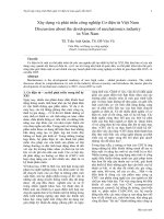
Fig. 1. Poverty incidence curves—Vietnam.

the minority groups of just under three quarters the average for the majority. The

incidence of poverty is calculated to be 60% for the Kinh and Chinese and 80% for the
minorities.8 Fig. 1 plots the poverty incidence curves giving the cumulative distribution
functions of per capita expenditures for every possible poverty line. It shows the
disparity in living standards more starkly and indicates first-order dominance. The result
that poverty incidence is higher among minority households is also robust to different
equivalent scales.9 Non-income indicators of poverty in Table 1 show the same pattern.
Education attainments are clearly lower on average for the minorities. A much higher
proportion belong to illiterate households Ž12% versus 3%.. For 27% of the minority but
only 12% of majority households, the most educated member had primary education,
while 53% of the latter had a member who attended high school compared to only 31%
of minority households.
Given our interest in the role of geographical disparities, it is also useful to examine
how community endowments vary across the groups. Table 2 presents means over both
groups on whether certain attributes, facilities, and services are found in a household’s
commune of residence as well as mean distances from the commune center to the closest
facilities. Access to infrastructure facilities and services tends to be worse for the

8
For details on the poverty lines see Dollar and Glewwe, 1998. When we use a lower cutoff point of
two-thirds of the poverty line the prevalence drops to 24% for the majority group and 45% for the ethnic
minorities.
9
We treated the original per capita poverty line Ž z . as the per capita expenditure needed to escape poverty
at average household size. So, the poverty line per equivalent single person is z n r nu where n is the average
household size and u is the size elasticity. At any given u —tested from 0 to 1 at intervals of 0.1—the poverty
ranking does not change.


D. Õan de Walle, D. Gunewardenar Journal of DeÕelopment Economics 65 (2001) 177–207


187

Table 2
Accessibility to facilities by ethnicity

Market in the commune
Periodic market
Distance to closest market Žkm.
Public transport
Radio station
Health care clinic
Distance to closest hospital Žkm.
Lower secondary school
Distance to closest lower secondary school Žkm.
Upper secondary school
Distance to closest upper secondary school Žkm.
Distance to district center Žkm.
Distance to closest post office Žkm.
Unskilled labor employment is available
Commercial enterprise exists

Majority ethnic groups

Minority ethnic groups

Mean

St. Dev.

Mean


St. Dev.

0.53
0.15
1.0
0.48
0.52
0.96
8.6
0.94
0.20
0.10
6.1
9.6
3.8
0.66
0.49

0.50
0.36
2.0
0.50
0.50
0.19
5.4
0.24
0.95
0.31
4.7

7.8
4.2
0.47
0.50

0.13
0.36
3.15
0.56
0.15
0.84
11.9
0.83
2.4
0.11
10.3
19.5
6.9
0.44
0.26

0.34
0.48
3.72
0.50
0.36
0.37
7.8
0.38
6.5

0.32
7.03
15.3
6.0
0.50
0.44

Note: Unless noted, the table gives the proportions of majority and minority households who live in communes
with each facility or attribute. For example, 53% of majority group households reside in a commune that has a
permanent market versus only 13% of ethnic minority households. The distance variables represent average
kilometers from a household’s commune center to the closest such facility.

minorities. For example, they are much less likely to live in a commune with a
permanent Žas opposed to a periodic. market, a radio station, a health care center and a
lower secondary school. Of course, these data tell us nothing about the quality of the
facilities, which could well also vary across communes. Distances to the closest facility
are also generally larger, with larger variance across communes. Interestingly, the
variance in community characteristics across geographic areas tends to be larger for
minority households. Finally, indicators of non-farm employment opportunities—
whether unskilled labor work is available and whether there is a large commercial
enterprise in the commune—are both higher communes where majority households
reside.
A look at household income sources further indicates less diversified livelihoods for
the minorities. Among minority households all but 26% Žstandard deviation of 2.0%.
derive their incomes solely from own-account farming activities, while 56% Žstandard
deviation of 1.0%. of majority households have non-farm incomes sources. The ethnic
majority more often combine farming with self-employment in non-farm enterprises or
wage-employment.

4. Econometric specification

Following the discussion in Section 2, household welfare is assumed to be a function
of household and community level endowments and other attributes. To explore its


188

D. Õan de Walle, D. Gunewardenar Journal of DeÕelopment Economics 65 (2001) 177–207

determinants, we regress the log of per capita expenditures ŽWi jk . for the ith household
in minority or majority group j living in commune k, against household characteristics
Ž X i jk . and geographic effects Žhi j .:
lnWi jk s b j X i jk q hi j q ´ i jk

Ž 3.

where ´ i jk is a random error term, orthogonal to the explanatory variables.
Household characteristics include demographics: proportions of children in the 0- to
6- and 7- to 16-year brackets; proportions of male and female adults; and a series of
dummy variables describing whether household structure consists of a single individual;
a couple; a couple with one, two, or three or more children; a three-generation
household; or some ‘other’ composition.10 A few variables are specific to the head of
household: age and age squared, and gender. We also include a dummy variable for
whether the household receives remittances from relatives abroad.11
Household human capital is measured as a series of dummy variables for the highest
education level of the member who has completed the most formal schooling. For
example, if the most educated member attended middle school, that dummy has a value
of one while all the others are zero. This specification allows us to measure the
incremental returns to extra years or levels of education. Education is assumed to be
pre-determined to current consumption. However, there could still be omitted variable
bias. For example, one likely omitted variable is the quality of education. Disparate

returns to schooling across the groups could be picking up either a difference in the
returns to quality, or a dissimilarity in how quality differences affect schooling quantity.
We return to this point below.
As noted in the Introduction, not speaking the national language could present a
severe handicap to minority households. Unfortunately, we are unable to test this
satisfactorily. The only indication of language skills in the questionnaire is that related to
whether Vietnamese was used for the VNLSS interview. This applies to virtually
everyone in the majority group Ž99.5%., and almost half of the minority households
Ž47.4%.. There is too little variance to include a language dummy variable in the
majority group regression Žthe effect is in the constant term., and, hence, this is not an
appropriate variable for the paper’s approach, which requires that the variables appear
jointly in both groups’ regressions. Out of interest, we did test a dummy variable for
language of interview in the minority regression. Contrary to expectations, we found it

10
There are concerns with assuming that the demographics are exogenous. However, one should also
recognize that per capita household expenditure may be an imperfect measure of welfare. For example, there
may be economies of scale in consumption or differences in needs for different age groups. Thus, demographic
controls are needed to deal with heterogeneity in welfare at given expenditures per person.
11
Note that, in as much as it is a dummy variable, it is not affected by differences in levels of remittances
among recipients. While there may nonetheless be endogeneity concerns about this variable, we believe it
would be worse to exclude it. The dummy could well proxy for important unobserved factors that affect
consumption, such as the household’s connections and political clout in the commune and at higher levels of
government.


D. Õan de Walle, D. Gunewardenar Journal of DeÕelopment Economics 65 (2001) 177–207

189


to be insignificant.12 These results probably indicate that language of interview is a poor
measure of a household’s Vietnamese language skills and should not be taken as
conclusive evidence that language is not important.
We also include as explanatory variables the total area of different types of land
cultivated by the household in the last 12 months. Land is disaggregated into area of
irrigated and non-irrigated annual crop land, perennial crop land, forest, water surface
Žmost often used for the culture of fish., and other land Žconsisting of vacant lots, bald
hills, burnt and fallow land, river banks, road and dike sides..13 To measure land quality,
we enter the shares of total irrigated and non-irrigated land recorded in the survey as
locally rated of good quality. Land markets did not exist at the time of data collection.
But even though households did not flexibly and freely choose land, the possibility of
endogeneity cannot be fully dismissed here either. Within communes, land allocations
were made by local administrations. Original household allocations of annual crop land
often date back to 1988 and were usually made on a per labor unit basis and allowing
for quality differentials and water access. Other land types Žperennial, forest and other
land. were distributed as late as 1991 or later, and appear to have frequently been
subject to greater local discretion.14 For example, Donovan et al. Ž1997. report great
variation in how the national land tenure regulations have been applied in the country’s
northern regions. They found that common criteria for distributing forest and other land
included evidence of sufficient household labor, capital, and ability to make investments.
They also describe numerous instances of apparent favoritism in forest and other land
allocation, with outcomes commonly favoring privileged village households.
The process of local land allocation suggests possible endogeneity, whereby some
land assets are a function of latent factors such as local political influence or access to
capital that also influence consumption but are not in the regression. The land coefficients then reflect both the returns to land and to those omitted variables. We will return
to this point when interpreting our results.
Finally, we include dummy variables for the commune in which the household lives.
As emphasized in Section 2, in this particular setting it can be argued that location is
largely exogenous and has a direct causal effect on living standards. Allowing for

commune fixed effects also helps deal with potential bias in other parameters of interest.
As also discussed in Section 2, latent factors that may be correlated with included
variables, and directly influence the dependent variable, are likely to be geographically
correlated. Communes are relatively small and the commune effects should adequately
capture differences in inter-commune quality of land and education attributes, local
infrastructure development, geo-environmental attributes, prices, and other community

12
It was insignificant everywhere except in the sample limited to communes where both groups are found,
without fixed effects. The effect disappeared when commune effects were entered.
13
Any swidden land that was cultivated during the last year is included in annual crop land. Swidden land is
more commonly cultivated by the minorities. Unfortunately, the survey does not collect information on area of
swidden land left fallow in the last year but available to the household.
14
For example, see the commune case studies reported in Donovan et al. Ž1997, vol. 2.. Also see Jamieson
Ž1996..


190

D. Õan de Walle, D. Gunewardenar Journal of DeÕelopment Economics 65 (2001) 177–207

level factors. This helps deal with the likely correlation between the included variables
—notably land and education—and location. Without geographical fixed effects a bias
is probable. There may of course still be some bias due to intra-commune differences in
omitted variables—including possible factors influencing within commune land allocations as noted above—but we can do nothing about this.
We run two sets of regressions. The first includes household level characteristics
excluding location. Since differences in the returns to those characteristics may well
reflect where one lives, we then run the regressions with commune fixed effects and test

for the influence of locational factors on the returns to household characteristics. In all
regressions, we estimate the standard errors using the Huber–White correction for
heteroscedasticity and we correct for the non-zero covariance within communes due to
sample design Žusing the robust cluster option in STATA 6..
5. Discussion of results
Table 3 presents the regression results for the majority and minority groups on the
full northern Viet Nam sample. Chow tests on these regressions reject the null
hypothesis that the parameters are the same for the two groups Ž F s 4.64 Ž34,84.. when
geographical fixed effects are excluded. Testing the joint restrictions Žincluding commune coefficients. is not possible when controlling for fixed effects since the number of
variables is now different in the two regressions as a result of both groups not being
found in all communes. However, we can still test for whether the coefficients on
household variables excluding location are the same; this test rejects the null that they
are Ž F s 36.48 Ž31,84... Table 4 gives the same regressions restricted to the sample of
704 households—366 majority and 338 minority—residing in mixed communes. Chow
tests also convincingly reject identical parameters both without and with fixed effects.15
The minority level regressions are rather similar for both samples, but some qualitative
differences arise in the majority group regressions. In general, the estimated parameters
in Table 4 have higher standard errors which would seem to support exploiting the
higher variance found in the larger sample. The discussion focuses on the regressions in
Table 3 since this is the full sample, representative of northern Viet Nam. Important
qualitative differences in the estimation performed on the sub-sample of mixed communes only are noted as we go along.
Subtracting the minority from the majority regression Žboth with commune effects.
tells us about the contribution to ethnic inequality of a change in specific household
attributes, controlling for commune of residence. The constant term—combining the
joint effects of excluded dummy variables—contributes positively to inequality between
the groups, as do the education variables, the receipt of remittances dummy, household
size, the household composition variables, the share of good quality irrigated land and
forest land. Other types of land, a male household head and household structures other
15
This is true using robust standard errors, both with and without cluster effects. However, on the model

estimated allowing for clustering, we can only test up to 21 constraints at a time Žequal to the number of
clusters minus one..


D. Õan de Walle, D. Gunewardenar Journal of DeÕelopment Economics 65 (2001) 177–207

191

than the left-out ‘couple,’ reduce inequality. The following discussion goes into more
detail.
5.1. Demographic effects
Although on balance the size of the demographic variable parameters favors the
majority group, demographic effects are similar across the groups and regressions with
and without fixed effects. Household size has a strong negative impact on welfare.
Compared with the omitted share of members aged under six, higher shares of all other
members have significant positive impacts on living standards. The household structure
variables have no apparent explanatory power with the exception of the negative effect
of being a one-child couple compared to a couple alone for the majority when we
control for location. This last effect disappears in the mixed commune sample.
5.2. Returns to education
Striking differences arise in the education parameter estimates. They are consistently
positive and significant for both groups but returns to education are substantially higher
for the minority in the regression not allowing for commune effects. An increment to per
capita consumption expenditures of 75% of original consumption is indicated as a result
of the most educated member completing primary schooling. The cumulative impact of
completing middle school is to raise per capita consumption by 84%, and of high school
to more than double it. By contrast, returns for the majority are, respectively: 22%, 34%
and 49% over original consumption per person. The cumulative advantages of education
to the ethnic minorities are maintained through vocational or university education,
though the returns are diminishing the higher the education level. Looking at the

non-fixed effects results, one might feel justified in concluding that as education
expands, this will in itself reduce and eliminate ethnic inequality, obviating any need to
target.
However, given the impediments to migration, a generalized policy of education
expansion is not the solution. Education is closely linked with where a minority
household resides, so that once one introduces the geographic effects, the results change
dramatically: differences in the returns to education between ethnic groups are reversed.
Although impacts on minority living standards remain positive and significant, their
magnitude declines to the point of being lower than those estimated for the majority for
all but primary schooling. By contrast, the majority parameter estimates are much less
affected by omitting the geographic effects. This is shown in Fig. 2 which plots the
cumulative returns to education relative to being illiterate for both groups with and
without the fixed effects. Note that the figure shows the proportionate gains to
consumption. Since the proportionate gains Žwith fixed effects. are higher for the
majority, and they are also on average richer, the level consumption gains from
education must be even higher for the majority.
In other words, we find that the differences in returns are strongly associated with
where a minority household lives. There are large unconditional returns to schooling to
minorities, but the difference upends when comparing ethnic minority and non-minority


192

D. Õan de Walle, D. Gunewardenar Journal of DeÕelopment Economics 65 (2001) 177–207

Table 3
Determinants of living standards Žfull sample.
Majority
Coefficient


Constant
13.12
Household size Žlog. y0.27
Proportion of
0.48
members 7–16
Proportion of
0.78
male adults
Proportion of
0.60
female adults
Single-member
y0.08
household
Couple and child
0.00
Couple and
0.07
two children
Couple and three
0.04
or more children
Three-generation
0.04
household
Other household type
0.02
Age of head
0.01

Age of head squared y0.00
Male household head
0.01

Minority
t-ratio Coefficient

Commune fixed effects
t-ratio Majority

Minority

Coefficient

t-ratio Coefficient

t-ratio

92.0
4.66
6.32

12.73
y0.29
0.25

43.15
3.23
1.84


13.35
y0.33
0.37

97.64
6.89
5.49

12.49
y0.4
0.25

32.68
3.91
2.21

7.19

0.85

3.89

0.60

6.75

0.60

3.33


5.97

0.50

3.01

0.41

4.12

0.36

2.30

0.96

0.004

0.02

y0.14

1.89

y0.12

0.49

0.06
1.19


0.06
0.11

0.41
0.71

y0.11
y0.05

2.26
0.84

0.04
0.04

0.42
0.27

0.61

0.12

0.66

y0.09

1.44

0.01


0.07

0.56

0.09

0.64

y0.06

1.05

0.07

0.54

0.30
2.47
2.49
0.40

0.13
0.005
y0.000
0.01

0.80
0.41
0.44

0.10

y0.07
0.01
y1.2ey4
0.02

1.24
3.17
3.12
0.69

0.12
0.01
y1.6ey4
0.06

0.84
1.06
1.11
1.15

Most educated:
1–5 years
primary education
Most educated:
1–3 years
middle school
Most educated:
1–4 years

high school
Most educated:
vocational education
Most educated:
university education

0.20

2.57

0.56

5.33

0.17

2.36

0.19

3.53

0.29

3.86

0.61

7.74


0.26

3.55

0.20

2.77

0.40

4.85

0.74

7.07

0.38

4.90

0.31

3.96

0.53

6.59

0.78


6.88

0.53

6.93

0.36

3.79

0.79

8.18

0.81

3.26

0.71

7.93

0.51

2.31

Irrigated land
Irrigated land
squared
Nonirrigated land

Nonirrigated land
squared
Perennial crop land
Perennial crop land
squared
Forest land

y3.2ey5
4.0ey9

1.40
2.54

1.3ey4
y8.9ey9

1.83
0.71

1.2ey5
1.4ey9

0.71
1.34

2.0ey4
y2.3ey8

4.06
3.09


y4.8ey6
1.0ey10

0.39
0.74

8.6ey6
y1.5ey10

0.50
0.28

8.6ey6
y9.5ey11

2.03
2.00

1.9ey5
y2.3ey10

0.83
0.30

3.8ey5
3.0ey10

1.33
0.21


5.9ey5
y3.0ey9

1.34
0.54

1.5ey5
2.3ey10

0.56
0.18

1.1ey4
y8.3ey9

1.94
1.31

0.12

1.6ey5

0.96

1.9ey5

1.99

1.7ey5


0.96

y1.4ey6


D. Õan de Walle, D. Gunewardenar Journal of DeÕelopment Economics 65 (2001) 177–207

193

Table 3 Ž continued .
Majority
Coefficient

Minority
t-ratio Coefficient

Commune fixed effects
t-ratio Majority
Coefficient

Forest land squared
3.3ey11
Water surface land
8.4ey5
Water surface land y4.4ey9
squared
Other land
y1.8ey5
Other land squared

3.2ey10
Proportion of
0.004
good quality
irrigated land
Proportion of
0.07
good quality
nonirrigated land
Income from
0.35
relatives abroad
Žyesrno.
Observations
F
Prob) F
R-squared
Root MSE

Minority
t-ratio Coefficient

t-ratio

0.13
2.88
2.42

y3.2ey10 0.63
4.0ey4 2.92

y2.2ey7 2.08

y4.7ey10 2.27
1.1ey4 3.68
y5.7ey9 2.94

y5.0ey10 0.98
3.8ey4 2.62
y1.8ey7 1.66

1.01
1.25
0.08

3.2ey6 0.21
1.1ey10 0.22
y0.05
0.46

5.4ey6 0.56
1.5ey11 0.11
0.03
0.89

2.5ey5 0.97
y5.6ey10 0.64
0.02
0.34

1.54


0.24

1.90

y0.01

0.25

0.20

2.74

4.57

0.34

3.49

0.27

5.40

0.24

4.82

2254
Ž28,80. s 27.44
0.0000

0.25
0.4007

466
Ž24,25. s119.81
0.0000
0.46
0.3833

2254
Ž32,80. s6975.05
0.0000
0.48
0.3398

466
Ž19,25. s 208.10
0.0000
0.61
0.3346

Note: the regression omits the proportion of members aged 0–6; households that consist of a couple; illiterate
education status. We leave out the commune fixed effects for ease of presentation. t-Ratios are estimated using
the robust cluster option in STATA 6.0 Ž1999..

households in the same place. The ethnic differences in unconditional returns thus arise
from the geographic distribution of ethnic groups such that the real difference between
high education, high consumption minority households and those with low education
and low consumption is in where they live. Under-developed labor markets and
considerable immobility allow this to happen.

These results suggest a substantial bias in the estimated returns to schooling for the
minorities when not controlling for commune effects. The key omitted characteristic is
likely to be the quality of education, which is itself determined geographically for the
minority group. Our results are consistent with a situation in which the places where
living standards are higher for the minority are places where education quality tends to
be better, and the latent quality differences are positively correlated with quantities of
education.16 However, we do not find a similar bias for the majority Žnoting that the
regressions with and without fixed effects are similar for the majority.. Either there are

16
Notice that both conditions are required. The omitted variable bias is the coefficient of the omitted
variable in the main regression times the regression coefficient of the excluded variable on the included
variable.


194

D. Õan de Walle, D. Gunewardenar Journal of DeÕelopment Economics 65 (2001) 177–207

Table 4
Determinants of living standards Žmixed communes only.
Majority
Coefficient

Minority
t-ratio Coefficient

Commune fixed effects
t-ratio Majority


Minority

Coefficient

t-ratio Coefficient

t-ratio

Constant
Household size Žlog.
Proportion of
members 7–16
Proportion of
male adults
Proportion of
female adults
Single-member
household
Couple and child
Couple and two
children
Couple and three
or more children
Three-generation
household
Other household type
Age of head
Age of head squared
Male household head


13.14
y0.44
0.50

44.97
2.85
2.61

13.05
y0.29
0.26

35.84
3.31
1.54

13.79
y0.37
0.28

46.31
2.95
1.53

13.33
y0.34
0.17

48.76
3.84

1.04

0.80

3.84

0.74

7.06

0.53

2.42

0.50

3.96

0.68

2.36

0.52

2.86

0.41

1.44


0.40

2.04

y0.06

0.40

0.14

0.48

y0.17

1.00

y0.02

0.08

0.10
0.19

1.07
1.80

y0.08
0.01

0.48

0.06

y0.11
y0.07

1.08
0.60

y0.13
y0.12

1.08
0.73

0.23

1.44

0.01

0.04

y0.07

0.53

y0.15

0.87


0.15

0.83

0.03

0.15

y0.10

0.69

y0.09

0.59

0.13
0.01
y8.8ey6
y0.40

1.34
0.40
0.06
0.37

0.09
0.01
y1.0ey4
0.06


0.58
0.70
0.75
1.08

y0.07
0.01
y4.5ey5
y0.02

0.73
0.60
0.37
0.20

y0.02
0.02
y2.4ey4
0.05

0.16
1.55
1.62
0.82

Most educated:
1–5 years
primary education
Most educated:

1–3 years
middle school
Most educated:
1–4 years high school
Most educated:
vocational education
Most educated:
university education

0.45

1.91

0.29

3.50

0.36

1.55

0.15

0.96

0.37

1.41

0.35


2.96

0.30

1.17

0.19

1.06

0.51

2.07

0.42

3.78

0.48

1.99

0.27

1.51

0.57

2.09


0.48

3.99

0.55

2.13

0.32

1.66

0.91

3.22

0.37

1.49

0.73

3.06

0.35

1.14

Irrigated land

Irrigated land squared
Nonirrigated land
Nonirrigated land
squared
Perennial crop land
Perennial crop land
squared
Forest land
Forest land squared
Water surface land

y8.6ey5
3.3ey8
y3.0ey5
y3.8ey10

0.97
2.14
2.99
3.54

1.3ey4
y1.1ey8
9.3ey7
8.4ey11

1.75
1.0ey4
0.83 y8.6ey9
0.06

3.9ey5
0.14 y4.7ey10

1.35
0.74
5.06
5.33

1.6ey4
y2.0ey8
y1.4ey6
1.4ey10

3.01
2.23
0.06
0.17

1.0ey4
y5.0ey9

2.89
1.32

4.3ey5
y2.8ey9

1.05
0.61


3.22
2.42

1.4ey4
y1.0ey8

2.24
1.63

y9.6ey6
7.4ey10
1.6ey4

0.39
0.78
0.69

1.6ey5
y3.3ey10
4.0ey4

0.92
0.59
2.78

0.47
0.16
2.36

1.6ey5

y4.2ey10
4.0ey4

0.94
0.81
2.82

1.3ey4
y9.6ey9
1.1ey5
1.6ey10
4.2ey4


D. Õan de Walle, D. Gunewardenar Journal of DeÕelopment Economics 65 (2001) 177–207

195

Table 4 Ž continued .
Majority

Minority

Coefficient t-ratio

Coefficient

Commune fixed effects
t-ratio


Majority

Minority

Coefficient t-ratio

Coefficient

t-ratio

Water surface land
squared
Other land
Other land squared
Proportion of
good quality
irrigated land
Proportion of
good quality
nonirrigated land
Income from
relatives abroad
Žyesrno.

y1.7ey8

0.74

y2.2ey7


2.09

y4.0ey8

2.24

y1.8ey7

1.71

y3.5ey5
6.5ey9
y0.06

0.65
1.24
0.57

y2.7ey7
1.9ey10
y0.07

0.02
0.44
0.68

y2.0ey5
4.4ey9
y0.15


0.44
0.97
1.74

5.5ey6
y1.4ey10
0.04

0.35
0.29
0.66

0.23

2.08

0.18

1.32

0.19

1.71

0.16

1.98

0.67


4.12

0.35

4.57

0.52

4.59

0.23

4.69

Observations
F
Prob) F
R-squared
Root MSE

366
Ž20,21. s 2200.5
0.0000
0.44
0.3770

338
Ž20,21. s 2143.7
0.0000
0.39

0.3387

366
Ž20,21. s 3450.8
0.0000
0.60
0.3271

338
Ž15,21. s132.4
0.0000
0.54
0.3054

Note: the regression omits the proportion of members aged 0–6; households that consist of a couple; illiterate
education status. We leave out the commune fixed effects for ease of presentation. t-Ratios are estimated using
the robust cluster option in STATA 6.0 Ž1999..

few quality differences for the majority, or the differences are uncorrelated with
differences in observed quantities. We cannot say which it is.
The seemingly high returns to minority education suggested by the model without
commune effects appear to be due not to education but to the combined effect of
restrictions on migration and geographical differences in the provision of education
services. These have simultaneously created large intra-commune differences in consumption and education levels for the minorities. This results in high estimated returns
to education Žwithout fixed effects., and suggests potentially large returns to minority
migration. The fact that this does not happen for majority households Žwhose mobility is
also restricted. suggests that the provision of education has been more equitable across
majority areas.17
Commune fixed effects have a similar impact on the mixed commune sample
regressions. Minority returns to education—though they are not higher than those for the


17
When we drop the receipt of income from relatives abroad dummy, the results are almost identical, but
with slightly higher returns to education for both groups. This is consistent with it proxying for omitted
indicators of, for example, political importance in the community. Leaving it in is likely to give better
estimates of the returns to education. The dummy is non-zero for only 3% of majority and 1% of minority
households. ŽDetails available from the authors..


196

D. Õan de Walle, D. Gunewardenar Journal of DeÕelopment Economics 65 (2001) 177–207

Fig. 2. Returns to education by ethnicity.

majority when not controlling for commune effects—undergo a proportionately larger
decline than the majority’s with commune effects. Large differences in the returns to
education remain—with minorities getting lower returns with and without fixed effects
on the smaller sample.18
5.3. Returns to land
Joint significance tests of the linear and quadratic terms show that perennial, water
surface, and irrigated land are significant at the 5% level in all regressions, except for
irrigated land in the minority without fixed effects, where it is significant at the 10%
level. Non-irrigated land has little explanatory power in any regressions. Other land is
significant Ž5% level. in both majority regressions, and in the minority fixed effects at
the 10% level. In addition, the forest land variables are significant in the majority fixed
effects Ž5%..
To see how the returns to land assets vary across the groups, we create Fig. 3a and b,
which Žanalogously to Fig. 2 for education. plots proportionate consumption gains for
different amounts of land relative to having no land. To deal with the different land

types, we create a land bundle Židentical for both groups. combining the relativities of
all land types at the mean. This bundle therefore contains a fixed share of Žgood and bad
quality. irrigated and non-irrigated land, and other land types and is expressed in
18
We cannot reject the null that the education coefficients are the same on the smaller sample of communes
where both groups live. Although the returns are higher for the majority with fixed effects, collinearity
between education and other regressors is no doubt raising the standard errors.


D. Õan de Walle, D. Gunewardenar Journal of DeÕelopment Economics 65 (2001) 177–207

197

Fig. 3. Ža. Returns to land by ethnicity. Žb. Returns to land by ethnicity Žmixed communes only..

different total amounts. Thus, using the parameter estimates for each group, we plot the
group-specific proportionate consumption gains from different quantities of land, holding quality constant.19 We first discuss the full sample results given in Fig. 3a.
19

At zero land, per capita consumption of the groups will differ. The graph should not be interpreted as
saying that the minorities have higher consumption at any given amount of land.


198

D. Õan de Walle, D. Gunewardenar Journal of DeÕelopment Economics 65 (2001) 177–207

The regression without geographic effects gives implausible results: returns to land
for the majority are actually negative. For both groups returns appear to be underestimated. These results are consistent with the land parameters in the regressions without
fixed effects picking up the effects of omitted cross-commune quality of land variations

that one would expect to be negatively correlated with quantities of land. If high quality
is associated with lower quantities of land across locations, then returns to land will be
underestimated unless one controls for commune effects. We also find that the marginal
returns to aggregate land are higher for the ethnic minority groups, especially controlling
for where they live.20 Analogously to Fig. 2, we note that the differences in the gains to
levels of consumption will be lower than the plotted proportionate gains since the
minority group is poorer. However, the gains in levels are still larger than for the
majority group given that the proportionate difference in returns to land Žwith fixed
effects. is so much larger than the proportionate difference in consumption.
The minorities obtain higher increments to consumption from extra land ceteris
paribus ŽFig. 3a.. This is the opposite of what we would expect if there was a bias due to
endogeneity of administrative land allocation, as discussed in Section 4. A priori, one
expects omitted attributes such as access to credit or political clout to be more strongly
correlated with land allocation for the majority group. When we examine individual land
types, we find similar patterns for all but forest land, where returns favor the majority.
The available evidence points to the allocation of forest land being more subject to
idiosyncratic household characteristics than other land types ŽDonovan et al., 1997.. The
returns to forest land may reflect an over-estimation of the coefficients due to latent
omitted variables. But this cannot explain our results for aggregate land.
Clearly, there must be one or more inputs that ethnic minority households supply in
greater quantity so as to obtain a larger output from the same land. What could that be?
The available evidence makes it implausible that the minority households are less credit
constrained at any given amount of land and generally have access to more productive
inputs such as machinery or extension services than the majority.21 One interpretation
for these findings is that minority households are working harder on their own land to
compensate for their lack of off-farm opportunities. In general, minority households
have lower levels of education, larger size, fewer children in school, fewer outside
non-farm economic opportunities, and face an even thinner labor market than others
given where they live. They then have little choice but to work harder on their land.22
20


We tested the results by running alternative specifications including one with total land, total land squared
and shares of each type of land making up the total to take into account land type and quality. The pattern
evidenced in Fig. 3 is closely repeated each time. We therefore stayed with our functional form as it is more
flexible, and, hence, econometrically preferred, than the alternatives.
21
Lower access is documented in, for example, MRDP et al. Ž1999., and Jamieson Ž1996..
22
There is a possible alternative explanation for the higher returns to land for the minorities. As mentioned,
more among the minority cultivate swidden land. If they also generate income from the unobserved swidden
land left fallow, then the results could reflect omitted variable bias. However, the direction of the bias will
depend on whether the area of fallow swidden land is positively or negatively correlated with currently
cultivated land area. A positive correlation would result in an overestimation of the returns to land and could
explain our results, while a negative correlation would underestimate returns. We think it unlikely that a
positive correlation is a general tendency.


D. Õan de Walle, D. Gunewardenar Journal of DeÕelopment Economics 65 (2001) 177–207

199

Mean hours worked on one’s own household farm from the survey data provide strong
corroboration for this interpretation. Converting yearly hours worked per household into
8-h day equivalents gives a mean of 397 days across the majority households versus 697
days for minority households.23 Unfortunately, we are unable to express time worked
per land area since the survey provides no information on labor time by land type.
Instead, we run a regression of the log of total hours worked on one’s farm for the entire
sample against land variables Žincluding squared terms and the land quality variables.
and a dummy taking the value one if the household is minority and zero otherwise. The
estimated coefficient is 0.45 Ž t s 4.75.. This suggests close to 50% higher labor time for

minority households at given amounts and quality of land.24
A likely contributory factor is that the minorities as a whole are more adept at
exploiting high-return, non-traditional, agricultural and forest products. This is likely to
require an intimate knowledge of the ecosystem, inputs and how remunerative certain
non-traditional and sometimes illegal products are. Minorities have often lived in the
same areas for generations. Their long confinement in these areas has no doubt fostered
a lot of specialized agro-environmental knowledge that helps to optimize land use and
maximize output. These effects are likely to be reinforced by the minority group’s lack
of more traditional alternatives, and greater inaccessibility and distance from public
interest and policing.
Thus, it can be argued that the forces that led to the high concentrations of minorities
in upland and mountainous areas may well have the effect that the marginal returns to
land are actually higher for them. In this case, as a result of the poorer ethnic group
experiencing lower access to off-farm work, reduced access to good quality flat land and
complementary inputs such as capital, it compensates in ways that result in higher
returns to land. Nonetheless, despite the minorities’ additional efforts and specialized
knowledge, their consumption remains lower.25
An interesting change in the structure of returns to land occurs when we focus solely
on the mixed commune sample. As can be seen in Table 4, there are some changes in
the majority regressions—forest land becomes insignificant and perennial land significant. Here too, returns are underestimated for both groups when not controlling for
commune effects. But when we do, minority returns to land fall absolutely while those
to the majority rise absolutely relative to that in the full sample, to a point where returns
to land are somewhat higher for the majority in the common commune sample. Fig. 3b
—analogously to Fig. 3a—summarizes the overall results. This difference with the full
23
Minority male adults work the equivalent of 271 eight-hour days; female adults 293; and children 133. For
the majority household members the averages are: 145, 188, and 65, respectively.
24
We tested a number of alternative specifications Žwithout the squared land terms; including all other
household characteristics; including commune dummies; limiting the sample to households in communes

where both groups live.. Without exception, we get strong positive and significant effects of minority
household status on hours of farm work.
25
An implication of the findings is that there are land transfers from majority to minority that would raise
average consumption over both groups, and enhance both efficiency and equity. Such trades are not occurring
given non-existent land markets. The administrative land allocation appears to be creating efficiency losses.
The situation is akin to the classic case of inequality impeding growth whereby the poor have higher marginal
returns because they cannot get inputs such as credit ŽBinswanger et al., 1995..


200

D. Õan de Walle, D. Gunewardenar Journal of DeÕelopment Economics 65 (2001) 177–207

Fig. 4. Returns to location by ethnicity.

sample may well be caused by selection bias, one source of which could be that in
places where both groups live, administrative land allocations or inputs favor the
majority. Communes with mixed populations appear to be untypical of northern Viet
Nam. Minority returns to land are higher over the sample as a whole. But despite the
minorities working longer hours at given land amounts and quality in mixed communes
as well, their returns are lower in communes where they compete with the majority.26
5.4. Returns to location
A similar comparison can be made of the estimated commune effects Žthe h ’s in Eq.
Ž3.., but only for the regression run on the sample of communes that are home to
households from both groups.27 Fig. 4 plots the commune coefficients estimated for the
majority against those estimated for the minority group. With very few exceptions,
returns to a specific geographic location are higher for the minorities. In a way similar to

26


In mixed communes, minority male adults work the equivalent of 258 eight-hour days, female adults 279,
and children 120, versus 174, 207, and 74, respectively, for the majority household members.
27
The coefficients are estimated relative to a left-out commune, and so change according to the omitted
communes.


D. Õan de Walle, D. Gunewardenar Journal of DeÕelopment Economics 65 (2001) 177–207

201

what we found for land, the minorities appear to be specializing and drawing greater
advantage from location attributes. As a result they achieve higher returns, compared to
the majority living in the same places. This partly, though only partly, compensates for
lower consumption.
5.5. Summarizing the regressions
We find that excluding commune effects results in severe omitted variable bias. This
reflects the fact that non-geographic variables tend to be geographically correlated.
Geography also independently affects living standards as indicated by significant
commune effects. Where you live matters much more to the ethnic minorities’ consumption levels than to the majority’s. Greater geographic variance in living standards exists
among minority households. Because omitted geographic variables for the minorities
tend to be more positively correlated with desirable household characteristics, omitting
the fixed effects tends to overestimate the returns to desirable household characteristics.
In the full sample, land is to some degree offsetting because its returns respond to added
effort and input by minority households—making up for their lack of outside income
earning opportunities in certain geographic areas. This does not hold for mixed
communes, where access to other inputs or quality differences appear to favor the
majority. There is also evidence of compensating effects of location. A component of
consumption is due purely to where a household resides. Average consumption is lower

for the minority groups but absolutely more of that consumption is due to where they
live.

6. Aggregate differences in returns
As we have seen, there are both positive and negative compensating influences on
ethnic inequality emanating from differences in the returns to the same characteristics.
We now ask how much, in aggregate, differences in returns account for differences in
living standards. We decompose the between-group difference in log per capita consumption expenditures using the methods discussed in Section 2. We use alternatively
the majority and minority parameters as reference weights. The decomposition is
undefined for the full sample with commune fixed effects because of the missing
parameter when only one group is present in the sample for a commune.28 It can be
done for the fixed effects model only on the sample limited to households living in
communes where both minority and majority are found. This decomposition also allows
us to test for the possibility that differences in characteristics across the full sample
reflect in part differences among the majority households across communes in which
very few minority households are found. Table 5 presents the results.
28

The decomposition is highly sensitive to the reference when the regressors are not observed for all groups.