Charu C. Aggarwal

Neural
Networks and
Deep Learning
A Textbook


Neural Networks and Deep Learning


Charu C. Aggarwal

Neural Networks and Deep
Learning
A Textbook

123


Charu C. Aggarwal
IBM T. J. Watson Research Center
International Business Machines
Yorktown Heights, NY, USA

ISBN 978-3-319-94462-3
ISBN 978-3-319-94463-0 (eBook)
/>Library of Congress Control Number: 2018947636
c Springer International Publishing AG, part of Springer Nature 2018
This work is subject to copyright. All rights are reserved by the Publisher, whether the whole or part of the material is
concerned, specifically the rights of translation, reprinting, reuse of illustrations, recitation, broadcasting, reproduction on

microfilms or in any other physical way, and transmission or information storage and retrieval, electronic adaptation, computer software, or by similar or dissimilar methodology now known or hereafter developed.
The use of general descriptive names, registered names, trademarks, service marks, etc. in this publication does not imply,
even in the absence of a specific statement, that such names are exempt from the relevant protective laws and regulations and
therefore free for general use.
The publisher, the authors and the editors are safe to assume that the advice and information in this book are believed to be
true and accurate at the date of publication. Neither the publisher nor the authors or the editors give a warranty, express or
implied, with respect to the material contained herein or for any errors or omissions that may have been made. The publisher
remains neutral with regard to jurisdictional claims in published maps and institutional affiliations.
This Springer imprint is published by the registered company Springer Nature Switzerland AG
The registered company address is: Gewerbestrasse 11, 6330 Cham, Switzerland


To my wife Lata, my daughter Sayani,
and my late parents Dr. Prem Sarup and Mrs. Pushplata Aggarwal.


Preface

“Any A.I. smart enough to pass a Turing test is smart enough to know to fail
it.”—Ian McDonald
Neural networks were developed to simulate the human nervous system for machine
learning tasks by treating the computational units in a learning model in a manner similar
to human neurons. The grand vision of neural networks is to create artificial intelligence
by building machines whose architecture simulates the computations in the human nervous system. This is obviously not a simple task because the computational power of the
fastest computer today is a minuscule fraction of the computational power of a human
brain. Neural networks were developed soon after the advent of computers in the fifties and
sixties. Rosenblatt’s perceptron algorithm was seen as a fundamental cornerstone of neural
networks, which caused an initial excitement about the prospects of artificial intelligence.
However, after the initial euphoria, there was a period of disappointment in which the data
hungry and computationally intensive nature of neural networks was seen as an impediment

to their usability. Eventually, at the turn of the century, greater data availability and increasing computational power lead to increased successes of neural networks, and this area
was reborn under the new label of “deep learning.” Although we are still far from the day
that artificial intelligence (AI) is close to human performance, there are specific domains
like image recognition, self-driving cars, and game playing, where AI has matched or exceeded human performance. It is also hard to predict what AI might be able to do in the
future. For example, few computer vision experts would have thought two decades ago that
any automated system could ever perform an intuitive task like categorizing an image more
accurately than a human.
Neural networks are theoretically capable of learning any mathematical function with
sufficient training data, and some variants like recurrent neural networks are known to be
Turing complete. Turing completeness refers to the fact that a neural network can simulate
any learning algorithm, given sufficient training data. The sticking point is that the amount
of data required to learn even simple tasks is often extraordinarily large, which causes a
corresponding increase in training time (if we assume that enough training data is available
in the first place). For example, the training time for image recognition, which is a simple
task for a human, can be on the order of weeks even on high-performance systems. Furthermore, there are practical issues associated with the stability of neural network training,
which are being resolved even today. Nevertheless, given that the speed of computers is
VII


VIII

PREFACE

expected to increase rapidly over time, and fundamentally more powerful paradigms like
quantum computing are on the horizon, the computational issue might not eventually turn
out to be quite as critical as imagined.
Although the biological analogy of neural networks is an exciting one and evokes comparisons with science fiction, the mathematical understanding of neural networks is a more
mundane one. The neural network abstraction can be viewed as a modular approach of
enabling learning algorithms that are based on continuous optimization on a computational
graph of dependencies between the input and output. To be fair, this is not very different

from traditional work in control theory; indeed, some of the methods used for optimization
in control theory are strikingly similar to (and historically preceded) the most fundamental
algorithms in neural networks. However, the large amounts of data available in recent years
together with increased computational power have enabled experimentation with deeper
architectures of these computational graphs than was previously possible. The resulting
success has changed the broader perception of the potential of deep learning.
The chapters of the book are organized as follows:
1. The basics of neural networks: Chapter 1 discusses the basics of neural network design.
Many traditional machine learning models can be understood as special cases of neural
learning. Understanding the relationship between traditional machine learning and
neural networks is the first step to understanding the latter. The simulation of various
machine learning models with neural networks is provided in Chapter 2. This will give
the analyst a feel of how neural networks push the envelope of traditional machine
learning algorithms.
2. Fundamentals of neural networks: Although Chapters 1 and 2 provide an overview
of the training methods for neural networks, a more detailed understanding of the
training challenges is provided in Chapters 3 and 4. Chapters 5 and 6 present radialbasis function (RBF) networks and restricted Boltzmann machines.
3. Advanced topics in neural networks: A lot of the recent success of deep learning is a
result of the specialized architectures for various domains, such as recurrent neural
networks and convolutional neural networks. Chapters 7 and 8 discuss recurrent and
convolutional neural networks. Several advanced topics like deep reinforcement learning, neural Turing mechanisms, and generative adversarial networks are discussed in
Chapters 9 and 10.
We have taken care to include some of the “forgotten” architectures like RBF networks
and Kohonen self-organizing maps because of their potential in many applications. The
book is written for graduate students, researchers, and practitioners. Numerous exercises
are available along with a solution manual to aid in classroom teaching. Where possible, an
application-centric view is highlighted in order to give the reader a feel for the technology.
Throughout this book, a vector or a multidimensional data point is annotated with a bar,
such as X or y. A vector or multidimensional point may be denoted by either small letters
or capital letters, as long as it has a bar. Vector dot products are denoted by centered dots,

such as X · Y . A matrix is denoted in capital letters without a bar, such as R. Throughout
the book, the n × d matrix corresponding to the entire training data set is denoted by
D, with n documents and d dimensions. The individual data points in D are therefore
d-dimensional row vectors. On the other hand, vectors with one component for each data


PREFACE

IX

point are usually n-dimensional column vectors. An example is the n-dimensional column
vector y of class variables of n data points. An observed value yi is distinguished from a
predicted value yˆi by a circumflex at the top of the variable.
Yorktown Heights, NY, USA

Charu C. Aggarwal


Acknowledgments

I would like to thank my family for their love and support during the busy time spent
in writing this book. I would also like to thank my manager Nagui Halim for his support
during the writing of this book.
Several figures in this book have been provided by the courtesy of various individuals
and institutions. The Smithsonian Institution made the image of the Mark I perceptron
(cf. Figure 1.5) available at no cost. Saket Sathe provided the outputs in Chapter 7 for
the tiny Shakespeare data set, based on code available/described in [233, 580]. Andrew
Zisserman provided Figures 8.12 and 8.16 in the section on convolutional visualizations.
Another visualization of the feature maps in the convolution network (cf. Figure 8.15) was
provided by Matthew Zeiler. NVIDIA provided Figure 9.10 on the convolutional neural

network for self-driving cars in Chapter 9, and Sergey Levine provided the image on selflearning robots (cf. Figure 9.9) in the same chapter. Alec Radford provided Figure 10.8,
which appears in Chapter 10. Alex Krizhevsky provided Figure 8.9(b) containing AlexNet.
This book has benefitted from significant feedback and several collaborations that I have
had with numerous colleagues over the years. I would like to thank Quoc Le, Saket Sathe,
Karthik Subbian, Jiliang Tang, and Suhang Wang for their feedback on various portions of
this book. Shuai Zheng provided feedbback on the section on regularized autoencoders in
Chapter 4. I received feedback on the sections on autoencoders from Lei Cai and Hao Yuan.
Feedback on the chapter on convolutional neural networks was provided by Hongyang Gao,
Shuiwang Ji, and Zhengyang Wang. Shuiwang Ji, Lei Cai, Zhengyang Wang and Hao Yuan
also reviewed the Chapters 3 and 7, and suggested several edits. They also suggested the
ideas of using Figures 8.6 and 8.7 for elucidating the convolution/deconvolution operations.
For their collaborations, I would like to thank Tarek F. Abdelzaher, Jinghui Chen, Jing
Gao, Quanquan Gu, Manish Gupta, Jiawei Han, Alexander Hinneburg, Thomas Huang,
Nan Li, Huan Liu, Ruoming Jin, Daniel Keim, Arijit Khan, Latifur Khan, Mohammad M.
Masud, Jian Pei, Magda Procopiuc, Guojun Qi, Chandan Reddy, Saket Sathe, Jaideep Srivastava, Karthik Subbian, Yizhou Sun, Jiliang Tang, Min-Hsuan Tsai, Haixun Wang, Jianyong Wang, Min Wang, Suhang Wang, Joel Wolf, Xifeng Yan, Mohammed Zaki, ChengXiang
Zhai, and Peixiang Zhao. I would also like to thank my advisor James B. Orlin for his guidance during my early years as a researcher.

XI


XII

ACKNOWLEDGMENTS

I would like to thank Lata Aggarwal for helping me with some of the figures created
using PowerPoint graphics in this book. My daughter, Sayani, was helpful in incorporating
special effects (e.g., image color, contrast, and blurring) in several JPEG images used at
various places in this book.



Contents

1 An Introduction to Neural Networks
1.1 Introduction . . . . . . . . . . . . . . . . . . . . . . . . . . . . . . . . . . .
1.1.1 Humans Versus Computers: Stretching the Limits
of Artificial Intelligence . . . . . . . . . . . . . . . . . . . . . . . .
1.2 The Basic Architecture of Neural Networks . . . . . . . . . . . . . . . . .
1.2.1 Single Computational Layer: The Perceptron . . . . . . . . . . . .
1.2.1.1 What Objective Function Is the Perceptron Optimizing?
1.2.1.2 Relationship with Support Vector Machines . . . . . . . .
1.2.1.3 Choice of Activation and Loss Functions . . . . . . . . .
1.2.1.4 Choice and Number of Output Nodes . . . . . . . . . . .
1.2.1.5 Choice of Loss Function . . . . . . . . . . . . . . . . . . .
1.2.1.6 Some Useful Derivatives of Activation Functions . . . . .
1.2.2 Multilayer Neural Networks . . . . . . . . . . . . . . . . . . . . . .
1.2.3 The Multilayer Network as a Computational Graph . . . . . . . .
1.3 Training a Neural Network with Backpropagation . . . . . . . . . . . . . .
1.4 Practical Issues in Neural Network Training . . . . . . . . . . . . . . . . .
1.4.1 The Problem of Overfitting . . . . . . . . . . . . . . . . . . . . . .
1.4.1.1 Regularization . . . . . . . . . . . . . . . . . . . . . . . .
1.4.1.2 Neural Architecture and Parameter Sharing . . . . . . . .
1.4.1.3 Early Stopping . . . . . . . . . . . . . . . . . . . . . . . .
1.4.1.4 Trading Off Breadth for Depth . . . . . . . . . . . . . . .
1.4.1.5 Ensemble Methods . . . . . . . . . . . . . . . . . . . . . .
1.4.2 The Vanishing and Exploding Gradient Problems . . . . . . . . . .
1.4.3 Difficulties in Convergence . . . . . . . . . . . . . . . . . . . . . . .
1.4.4 Local and Spurious Optima . . . . . . . . . . . . . . . . . . . . . .
1.4.5 Computational Challenges . . . . . . . . . . . . . . . . . . . . . . .
1.5 The Secrets to the Power of Function Composition . . . . . . . . . . . . .
1.5.1 The Importance of Nonlinear Activation . . . . . . . . . . . . . . .

1.5.2 Reducing Parameter Requirements with Depth . . . . . . . . . . .
1.5.3 Unconventional Neural Architectures . . . . . . . . . . . . . . . . .
1.5.3.1 Blurring the Distinctions Between Input, Hidden,
and Output Layers . . . . . . . . . . . . . . . . . . . . . .
1.5.3.2 Unconventional Operations and Sum-Product Networks .

.

1
1

.
.
.
.
.
.
.
.
.
.
.
.
.
.
.
.
.
.
.

.
.
.
.
.
.
.
.

3
4
5
8
10
11
14
14
16
17
20
21
24
25
26
27
27
27
28
28
29

29
29
30
32
34
35

.
.

35
36
XIII


XIV

1.6

CONTENTS

Common Neural Architectures . . . . . . . . . . . . . . . . . . .
1.6.1 Simulating Basic Machine Learning with Shallow Models
1.6.2 Radial Basis Function Networks . . . . . . . . . . . . . .
1.6.3 Restricted Boltzmann Machines . . . . . . . . . . . . . . .
1.6.4 Recurrent Neural Networks . . . . . . . . . . . . . . . . .
1.6.5 Convolutional Neural Networks . . . . . . . . . . . . . . .
1.6.6 Hierarchical Feature Engineering and Pretrained Models .
1.7 Advanced Topics . . . . . . . . . . . . . . . . . . . . . . . . . . .
1.7.1 Reinforcement Learning . . . . . . . . . . . . . . . . . . .

1.7.2 Separating Data Storage and Computations . . . . . . . .
1.7.3 Generative Adversarial Networks . . . . . . . . . . . . . .
1.8 Two Notable Benchmarks . . . . . . . . . . . . . . . . . . . . . .
1.8.1 The MNIST Database of Handwritten Digits . . . . . . .
1.8.2 The ImageNet Database . . . . . . . . . . . . . . . . . . .
1.9 Summary . . . . . . . . . . . . . . . . . . . . . . . . . . . . . . .
1.10 Bibliographic Notes . . . . . . . . . . . . . . . . . . . . . . . . . .
1.10.1 Video Lectures . . . . . . . . . . . . . . . . . . . . . . . .
1.10.2 Software Resources . . . . . . . . . . . . . . . . . . . . . .
1.11 Exercises . . . . . . . . . . . . . . . . . . . . . . . . . . . . . . .

.
.
.
.
.
.
.
.
.
.
.
.
.
.
.
.
.
.
.


.
.
.
.
.
.
.
.
.
.
.
.
.
.
.
.
.
.
.

.
.
.
.
.
.
.
.
.

.
.
.
.
.
.
.
.
.
.

.
.
.
.
.
.
.
.
.
.
.
.
.
.
.
.
.
.
.


.
.
.
.
.
.
.
.
.
.
.
.
.
.
.
.
.
.
.

.
.
.
.
.
.
.
.
.

.
.
.
.
.
.
.
.
.
.

37
37
37
38
38
40
42
44
44
45
45
46
46
47
48
48
50
50
51


2 Machine Learning with Shallow Neural Networks
2.1 Introduction . . . . . . . . . . . . . . . . . . . . . . . . . . . . . .
2.2 Neural Architectures for Binary Classification Models . . . . . .
2.2.1 Revisiting the Perceptron . . . . . . . . . . . . . . . . . .
2.2.2 Least-Squares Regression . . . . . . . . . . . . . . . . . .
2.2.2.1 Widrow-Hoff Learning . . . . . . . . . . . . . . .
2.2.2.2 Closed Form Solutions . . . . . . . . . . . . . . .
2.2.3 Logistic Regression . . . . . . . . . . . . . . . . . . . . . .
2.2.3.1 Alternative Choices of Activation and Loss . . .
2.2.4 Support Vector Machines . . . . . . . . . . . . . . . . . .
2.3 Neural Architectures for Multiclass Models . . . . . . . . . . . .
2.3.1 Multiclass Perceptron . . . . . . . . . . . . . . . . . . . .
2.3.2 Weston-Watkins SVM . . . . . . . . . . . . . . . . . . . .
2.3.3 Multinomial Logistic Regression (Softmax Classifier) . . .
2.3.4 Hierarchical Softmax for Many Classes . . . . . . . . . . .
2.4 Backpropagated Saliency for Feature Selection . . . . . . . . . .
2.5 Matrix Factorization with Autoencoders . . . . . . . . . . . . . .
2.5.1 Autoencoder: Basic Principles . . . . . . . . . . . . . . . .
2.5.1.1 Autoencoder with a Single Hidden Layer . . . .
2.5.1.2 Connections with Singular Value Decomposition
2.5.1.3 Sharing Weights in Encoder and Decoder . . . .
2.5.1.4 Other Matrix Factorization Methods . . . . . . .
2.5.2 Nonlinear Activations . . . . . . . . . . . . . . . . . . . .
2.5.3 Deep Autoencoders . . . . . . . . . . . . . . . . . . . . . .
2.5.4 Application to Outlier Detection . . . . . . . . . . . . . .
2.5.5 When the Hidden Layer Is Broader than the Input Layer
2.5.5.1 Sparse Feature Learning . . . . . . . . . . . . . .
2.5.6 Other Applications . . . . . . . . . . . . . . . . . . . . . .


.
.
.
.
.
.
.
.
.
.
.
.
.
.
.
.
.
.
.
.
.
.
.
.
.
.
.

.
.

.
.
.
.
.
.
.
.
.
.
.
.
.
.
.
.
.
.
.
.
.
.
.
.
.

.
.
.
.

.
.
.
.
.
.
.
.
.
.
.
.
.
.
.
.
.
.
.
.
.
.
.

.
.
.
.
.
.

.
.
.
.
.
.
.
.
.
.
.
.
.
.
.
.
.
.
.
.
.

.
.
.
.
.
.
.
.

.
.
.
.
.
.
.
.
.
.
.
.
.
.
.
.
.
.
.

.
.
.
.
.
.
.
.
.
.

.
.
.
.
.
.
.
.
.
.
.
.
.
.
.
.
.

53
53
55
56
58
59
61
61
63
63
65
65

67
68
69
70
70
71
72
74
74
76
76
78
80
81
81
82


CONTENTS

XV

2.5.7 Recommender Systems: Row Index to Row Value Prediction
2.5.8 Discussion . . . . . . . . . . . . . . . . . . . . . . . . . . . . .
2.6 Word2vec: An Application of Simple Neural Architectures . . . . . .
2.6.1 Neural Embedding with Continuous Bag of Words . . . . . .
2.6.2 Neural Embedding with Skip-Gram Model . . . . . . . . . . .
2.6.3 Word2vec (SGNS) Is Logistic Matrix Factorization . . . . . .
2.6.4 Vanilla Skip-Gram Is Multinomial Matrix Factorization . . .
2.7 Simple Neural Architectures for Graph Embeddings . . . . . . . . .

2.7.1 Handling Arbitrary Edge Counts . . . . . . . . . . . . . . . .
2.7.2 Multinomial Model . . . . . . . . . . . . . . . . . . . . . . . .
2.7.3 Connections with DeepWalk and Node2vec . . . . . . . . . .
2.8 Summary . . . . . . . . . . . . . . . . . . . . . . . . . . . . . . . . .
2.9 Bibliographic Notes . . . . . . . . . . . . . . . . . . . . . . . . . . . .
2.9.1 Software Resources . . . . . . . . . . . . . . . . . . . . . . . .
2.10 Exercises . . . . . . . . . . . . . . . . . . . . . . . . . . . . . . . . .

.
.
.
.
.
.
.
.
.
.
.
.
.
.
.

.
.
.
.
.
.

.
.
.
.
.
.
.
.
.

.
.
.
.
.
.
.
.
.
.
.
.
.
.
.

.
.
.
.

.
.
.
.
.
.
.
.
.
.
.

83
86
87
87
90
95
98
98
100
100
100
101
101
102
103

3 Training Deep Neural Networks
3.1 Introduction . . . . . . . . . . . . . . . . . . . . . . . . . . . . . . . .

3.2 Backpropagation: The Gory Details . . . . . . . . . . . . . . . . . . .
3.2.1 Backpropagation with the Computational Graph Abstraction
3.2.2 Dynamic Programming to the Rescue . . . . . . . . . . . . .
3.2.3 Backpropagation with Post-Activation Variables . . . . . . .
3.2.4 Backpropagation with Pre-activation Variables . . . . . . . .
3.2.5 Examples of Updates for Various Activations . . . . . . . . .
3.2.5.1 The Special Case of Softmax . . . . . . . . . . . . .
3.2.6 A Decoupled View of Vector-Centric Backpropagation . . . .
3.2.7 Loss Functions on Multiple Output Nodes and Hidden Nodes
3.2.8 Mini-Batch Stochastic Gradient Descent . . . . . . . . . . . .
3.2.9 Backpropagation Tricks for Handling Shared Weights . . . .
3.2.10 Checking the Correctness of Gradient Computation . . . . .
3.3 Setup and Initialization Issues . . . . . . . . . . . . . . . . . . . . . .
3.3.1 Tuning Hyperparameters . . . . . . . . . . . . . . . . . . . .
3.3.2 Feature Preprocessing . . . . . . . . . . . . . . . . . . . . . .
3.3.3 Initialization . . . . . . . . . . . . . . . . . . . . . . . . . . .
3.4 The Vanishing and Exploding Gradient Problems . . . . . . . . . . .
3.4.1 Geometric Understanding of the Effect of Gradient Ratios . .
3.4.2 A Partial Fix with Activation Function Choice . . . . . . . .
3.4.3 Dying Neurons and “Brain Damage” . . . . . . . . . . . . . .
3.4.3.1 Leaky ReLU . . . . . . . . . . . . . . . . . . . . . .
3.4.3.2 Maxout . . . . . . . . . . . . . . . . . . . . . . . . .
3.5 Gradient-Descent Strategies . . . . . . . . . . . . . . . . . . . . . . .
3.5.1 Learning Rate Decay . . . . . . . . . . . . . . . . . . . . . . .
3.5.2 Momentum-Based Learning . . . . . . . . . . . . . . . . . . .
3.5.2.1 Nesterov Momentum . . . . . . . . . . . . . . . . .
3.5.3 Parameter-Specific Learning Rates . . . . . . . . . . . . . . .
3.5.3.1 AdaGrad . . . . . . . . . . . . . . . . . . . . . . . .
3.5.3.2 RMSProp . . . . . . . . . . . . . . . . . . . . . . . .
3.5.3.3 RMSProp with Nesterov Momentum . . . . . . . . .


.
.
.
.
.
.
.
.
.
.
.
.
.
.
.
.
.
.
.
.
.
.
.
.
.
.
.
.
.

.
.

.
.
.
.
.
.
.
.
.
.
.
.
.
.
.
.
.
.
.
.
.
.
.
.
.
.
.

.
.
.
.

.
.
.
.
.
.
.
.
.
.
.
.
.
.
.
.
.
.
.
.
.
.
.
.
.

.
.
.
.
.
.

.
.
.
.
.
.
.
.
.
.
.
.
.
.
.
.
.
.
.
.
.
.
.

.
.
.
.
.
.
.
.

105
105
107
107
111
113
115
117
117
118
121
121
123
124
125
125
126
128
129
130
133

133
133
134
134
135
136
137
137
138
138
139


XVI

CONTENTS

3.5.3.4 AdaDelta . . . . . . . . . . . . . . . . . . . . . . . . .
3.5.3.5 Adam . . . . . . . . . . . . . . . . . . . . . . . . . . .
3.5.4 Cliffs and Higher-Order Instability . . . . . . . . . . . . . . . .
3.5.5 Gradient Clipping . . . . . . . . . . . . . . . . . . . . . . . . .
3.5.6 Second-Order Derivatives . . . . . . . . . . . . . . . . . . . . .
3.5.6.1 Conjugate Gradients and Hessian-Free Optimization .
3.5.6.2 Quasi-Newton Methods and BFGS . . . . . . . . . . .
3.5.6.3 Problems with Second-Order Methods: Saddle Points
3.5.7 Polyak Averaging . . . . . . . . . . . . . . . . . . . . . . . . . .
3.5.8 Local and Spurious Minima . . . . . . . . . . . . . . . . . . . .
3.6 Batch Normalization . . . . . . . . . . . . . . . . . . . . . . . . . . . .
3.7 Practical Tricks for Acceleration and Compression . . . . . . . . . . .
3.7.1 GPU Acceleration . . . . . . . . . . . . . . . . . . . . . . . . .

3.7.2 Parallel and Distributed Implementations . . . . . . . . . . . .
3.7.3 Algorithmic Tricks for Model Compression . . . . . . . . . . .
3.8 Summary . . . . . . . . . . . . . . . . . . . . . . . . . . . . . . . . . .
3.9 Bibliographic Notes . . . . . . . . . . . . . . . . . . . . . . . . . . . . .
3.9.1 Software Resources . . . . . . . . . . . . . . . . . . . . . . . . .
3.10 Exercises . . . . . . . . . . . . . . . . . . . . . . . . . . . . . . . . . .
4 Teaching Deep Learners to Generalize
4.1 Introduction . . . . . . . . . . . . . . . . . . . . . . . . . . . . . . . .
4.2 The Bias-Variance Trade-Off . . . . . . . . . . . . . . . . . . . . . .
4.2.1 Formal View . . . . . . . . . . . . . . . . . . . . . . . . . . .
4.3 Generalization Issues in Model Tuning and Evaluation . . . . . . . .
4.3.1 Evaluating with Hold-Out and Cross-Validation . . . . . . . .
4.3.2 Issues with Training at Scale . . . . . . . . . . . . . . . . . .
4.3.3 How to Detect Need to Collect More Data . . . . . . . . . . .
4.4 Penalty-Based Regularization . . . . . . . . . . . . . . . . . . . . . .
4.4.1 Connections with Noise Injection . . . . . . . . . . . . . . . .
4.4.2 L1 -Regularization . . . . . . . . . . . . . . . . . . . . . . . .
4.4.3 L1 - or L2 -Regularization? . . . . . . . . . . . . . . . . . . . .
4.4.4 Penalizing Hidden Units: Learning Sparse Representations . .
4.5 Ensemble Methods . . . . . . . . . . . . . . . . . . . . . . . . . . . .
4.5.1 Bagging and Subsampling . . . . . . . . . . . . . . . . . . . .
4.5.2 Parametric Model Selection and Averaging . . . . . . . . . .
4.5.3 Randomized Connection Dropping . . . . . . . . . . . . . . .
4.5.4 Dropout . . . . . . . . . . . . . . . . . . . . . . . . . . . . . .
4.5.5 Data Perturbation Ensembles . . . . . . . . . . . . . . . . . .
4.6 Early Stopping . . . . . . . . . . . . . . . . . . . . . . . . . . . . . .
4.6.1 Understanding Early Stopping from the Variance Perspective
4.7 Unsupervised Pretraining . . . . . . . . . . . . . . . . . . . . . . . .
4.7.1 Variations of Unsupervised Pretraining . . . . . . . . . . . . .
4.7.2 What About Supervised Pretraining? . . . . . . . . . . . . .

4.8 Continuation and Curriculum Learning . . . . . . . . . . . . . . . . .
4.8.1 Continuation Learning . . . . . . . . . . . . . . . . . . . . . .
4.8.2 Curriculum Learning . . . . . . . . . . . . . . . . . . . . . . .
4.9 Parameter Sharing . . . . . . . . . . . . . . . . . . . . . . . . . . . .

.
.
.
.
.
.
.
.
.
.
.
.
.
.
.
.
.
.
.
.
.
.
.
.
.

.
.

.
.
.
.
.
.
.
.
.
.
.
.
.
.
.
.
.
.
.

.
.
.
.
.
.
.

.
.
.
.
.
.
.
.
.
.
.
.

.
.
.
.
.
.
.
.
.
.
.
.
.
.
.
.
.

.
.

139
140
141
142
143
145
148
149
151
151
152
156
157
158
160
163
163
165
165

.
.
.
.
.
.
.

.
.
.
.
.
.
.
.
.
.
.
.
.
.
.
.
.
.
.
.

.
.
.
.
.
.
.
.
.

.
.
.
.
.
.
.
.
.
.
.
.
.
.
.
.
.
.

.
.
.
.
.
.
.
.
.
.
.

.
.
.
.
.
.
.
.
.
.
.
.
.
.
.
.

169
169
174
175
178
179
180
181
181
182
183
184
185

186
186
187
188
188
191
192
192
193
197
197
199
199
200
200


CONTENTS

XVII

4.10 Regularization in Unsupervised Applications . . . . . . . . . . . . .
4.10.1 Value-Based Penalization: Sparse Autoencoders . . . . . . . .
4.10.2 Noise Injection: De-noising Autoencoders . . . . . . . . . . .
4.10.3 Gradient-Based Penalization: Contractive Autoencoders . . .
4.10.4 Hidden Probabilistic Structure: Variational Autoencoders . .
4.10.4.1 Reconstruction and Generative Sampling . . . . . .
4.10.4.2 Conditional Variational Autoencoders . . . . . . . .
4.10.4.3 Relationship with Generative Adversarial Networks
4.11 Summary . . . . . . . . . . . . . . . . . . . . . . . . . . . . . . . . .

4.12 Bibliographic Notes . . . . . . . . . . . . . . . . . . . . . . . . . . . .
4.12.1 Software Resources . . . . . . . . . . . . . . . . . . . . . . . .
4.13 Exercises . . . . . . . . . . . . . . . . . . . . . . . . . . . . . . . . .
5 Radial Basis Function Networks
5.1 Introduction . . . . . . . . . . . . . . . . . . . . . . . . . . . .
5.2 Training an RBF Network . . . . . . . . . . . . . . . . . . . .
5.2.1 Training the Hidden Layer . . . . . . . . . . . . . . . .
5.2.2 Training the Output Layer . . . . . . . . . . . . . . .
5.2.2.1 Expression with Pseudo-Inverse . . . . . . .
5.2.3 Orthogonal Least-Squares Algorithm . . . . . . . . . .
5.2.4 Fully Supervised Learning . . . . . . . . . . . . . . . .
5.3 Variations and Special Cases of RBF Networks . . . . . . . .
5.3.1 Classification with Perceptron Criterion . . . . . . . .
5.3.2 Classification with Hinge Loss . . . . . . . . . . . . . .
5.3.3 Example of Linear Separability Promoted by RBF . .
5.3.4 Application to Interpolation . . . . . . . . . . . . . . .
5.4 Relationship with Kernel Methods . . . . . . . . . . . . . . .
5.4.1 Kernel Regression as a Special Case of RBF Networks
5.4.2 Kernel SVM as a Special Case of RBF Networks . . .
5.4.3 Observations . . . . . . . . . . . . . . . . . . . . . . .
5.5 Summary . . . . . . . . . . . . . . . . . . . . . . . . . . . . .
5.6 Bibliographic Notes . . . . . . . . . . . . . . . . . . . . . . . .
5.7 Exercises . . . . . . . . . . . . . . . . . . . . . . . . . . . . .

.
.
.
.
.
.

.
.
.
.
.
.

.
.
.
.
.
.
.
.
.
.
.
.

.
.
.
.
.
.
.
.
.
.

.
.

.
.
.
.
.
.
.
.
.
.
.
.

201
202
202
204
207
210
212
213
213
214
215
215

.

.
.
.
.
.
.
.
.
.
.
.
.
.
.
.
.
.
.

.
.
.
.
.
.
.
.
.
.
.

.
.
.
.
.
.
.
.

.
.
.
.
.
.
.
.
.
.
.
.
.
.
.
.
.
.
.

.

.
.
.
.
.
.
.
.
.
.
.
.
.
.
.
.
.
.

.
.
.
.
.
.
.
.
.
.
.

.
.
.
.
.
.
.
.

.
.
.
.
.
.
.
.
.
.
.
.
.
.
.
.
.
.
.

.

.
.
.
.
.
.
.
.
.
.
.
.
.
.
.
.
.
.

217
217
220
221
222
224
224
225
226
226
227

227
228
229
229
230
231
231
232
232

6 Restricted Boltzmann Machines
6.1 Introduction . . . . . . . . . . . . . . . . . . . . . . . . . . . . . .
6.1.1 Historical Perspective . . . . . . . . . . . . . . . . . . . .
6.2 Hopfield Networks . . . . . . . . . . . . . . . . . . . . . . . . . .
6.2.1 Optimal State Configurations of a Trained Network . . .
6.2.2 Training a Hopfield Network . . . . . . . . . . . . . . . .
6.2.3 Building a Toy Recommender and Its Limitations . . . .
6.2.4 Increasing the Expressive Power of the Hopfield Network
6.3 The Boltzmann Machine . . . . . . . . . . . . . . . . . . . . . . .
6.3.1 How a Boltzmann Machine Generates Data . . . . . . . .
6.3.2 Learning the Weights of a Boltzmann Machine . . . . . .
6.4 Restricted Boltzmann Machines . . . . . . . . . . . . . . . . . . .
6.4.1 Training the RBM . . . . . . . . . . . . . . . . . . . . . .
6.4.2 Contrastive Divergence Algorithm . . . . . . . . . . . . .
6.4.3 Practical Issues and Improvisations . . . . . . . . . . . . .

.
.
.
.

.
.
.
.
.
.
.
.
.
.

.
.
.
.
.
.
.
.
.
.
.
.
.
.

.
.
.
.

.
.
.
.
.
.
.
.
.
.

.
.
.
.
.
.
.
.
.
.
.
.
.
.

.
.
.
.

.
.
.
.
.
.
.
.
.
.

.
.
.
.
.
.
.
.
.
.
.
.
.
.

235
235
236
237

238
240
241
242
243
244
245
247
249
250
251

.
.
.
.
.
.
.
.
.
.
.
.
.
.
.
.
.
.

.


XVIII

6.5

Applications of Restricted Boltzmann Machines . . . . . . . .
6.5.1 Dimensionality Reduction and Data Reconstruction .
6.5.2 RBMs for Collaborative Filtering . . . . . . . . . . . .
6.5.3 Using RBMs for Classification . . . . . . . . . . . . . .
6.5.4 Topic Models with RBMs . . . . . . . . . . . . . . . .
6.5.5 RBMs for Machine Learning with Multimodal Data .
6.6 Using RBMs Beyond Binary Data Types . . . . . . . . . . . .
6.7 Stacking Restricted Boltzmann Machines . . . . . . . . . . .
6.7.1 Unsupervised Learning . . . . . . . . . . . . . . . . . .
6.7.2 Supervised Learning . . . . . . . . . . . . . . . . . . .
6.7.3 Deep Boltzmann Machines and Deep Belief Networks
6.8 Summary . . . . . . . . . . . . . . . . . . . . . . . . . . . . .
6.9 Bibliographic Notes . . . . . . . . . . . . . . . . . . . . . . . .
6.10 Exercises . . . . . . . . . . . . . . . . . . . . . . . . . . . . .

CONTENTS

.
.
.
.
.
.

.
.
.
.
.
.
.
.

.
.
.
.
.
.
.
.
.
.
.
.
.
.

.
.
.
.
.
.

.
.
.
.
.
.
.
.

.
.
.
.
.
.
.
.
.
.
.
.
.
.

.
.
.
.
.
.

.
.
.
.
.
.
.
.

.
.
.
.
.
.
.
.
.
.
.
.
.
.

.
.
.
.
.
.

.
.
.
.
.
.
.
.

.
.
.
.
.
.
.
.
.
.
.
.
.
.

251
252
254
257
260
262

263
264
266
267
267
268
268
270

7 Recurrent Neural Networks
7.1 Introduction . . . . . . . . . . . . . . . . . . . . . . . . . . . . . .
7.1.1 Expressiveness of Recurrent Networks . . . . . . . . . . .
7.2 The Architecture of Recurrent Neural Networks . . . . . . . . . .
7.2.1 Language Modeling Example of RNN . . . . . . . . . . .
7.2.1.1 Generating a Language Sample . . . . . . . . . .
7.2.2 Backpropagation Through Time . . . . . . . . . . . . . .
7.2.3 Bidirectional Recurrent Networks . . . . . . . . . . . . . .
7.2.4 Multilayer Recurrent Networks . . . . . . . . . . . . . . .
7.3 The Challenges of Training Recurrent Networks . . . . . . . . . .
7.3.1 Layer Normalization . . . . . . . . . . . . . . . . . . . . .
7.4 Echo-State Networks . . . . . . . . . . . . . . . . . . . . . . . . .
7.5 Long Short-Term Memory (LSTM) . . . . . . . . . . . . . . . . .
7.6 Gated Recurrent Units (GRUs) . . . . . . . . . . . . . . . . . . .
7.7 Applications of Recurrent Neural Networks . . . . . . . . . . . .
7.7.1 Application to Automatic Image Captioning . . . . . . . .
7.7.2 Sequence-to-Sequence Learning and Machine Translation
7.7.2.1 Question-Answering Systems . . . . . . . . . . .
7.7.3 Application to Sentence-Level Classification . . . . . . . .
7.7.4 Token-Level Classification with Linguistic Features . . . .
7.7.5 Time-Series Forecasting and Prediction . . . . . . . . . .

7.7.6 Temporal Recommender Systems . . . . . . . . . . . . . .
7.7.7 Secondary Protein Structure Prediction . . . . . . . . . .
7.7.8 End-to-End Speech Recognition . . . . . . . . . . . . . . .
7.7.9 Handwriting Recognition . . . . . . . . . . . . . . . . . .
7.8 Summary . . . . . . . . . . . . . . . . . . . . . . . . . . . . . . .
7.9 Bibliographic Notes . . . . . . . . . . . . . . . . . . . . . . . . . .
7.9.1 Software Resources . . . . . . . . . . . . . . . . . . . . . .
7.10 Exercises . . . . . . . . . . . . . . . . . . . . . . . . . . . . . . .

.
.
.
.
.
.
.
.
.
.
.
.
.
.
.
.
.
.
.
.
.

.
.
.
.
.
.
.

.
.
.
.
.
.
.
.
.
.
.
.
.
.
.
.
.
.
.
.
.
.

.
.
.
.
.
.

.
.
.
.
.
.
.
.
.
.
.
.
.
.
.
.
.
.
.
.
.
.
.

.
.
.
.
.

.
.
.
.
.
.
.
.
.
.
.
.
.
.
.
.
.
.
.
.
.
.
.
.

.
.
.
.

.
.
.
.
.
.
.
.
.
.
.
.
.
.
.
.
.
.
.
.
.
.
.
.
.

.
.
.

.
.
.
.
.
.
.
.
.
.
.
.
.
.
.
.
.
.
.
.
.
.
.
.
.
.

.
.

271
271
274
274
277
278
280
283
284
286
289
290
292
295
297
298
299
301
303
304
305
307
309
309
309
310
310

311
312


CONTENTS

XIX

8 Convolutional Neural Networks
8.1 Introduction . . . . . . . . . . . . . . . . . . . . . . . . . . . . . . . . . .
8.1.1 Historical Perspective and Biological Inspiration . . . . . . . . .
8.1.2 Broader Observations About Convolutional Neural Networks . .
8.2 The Basic Structure of a Convolutional Network . . . . . . . . . . . . .
8.2.1 Padding . . . . . . . . . . . . . . . . . . . . . . . . . . . . . . . .
8.2.2 Strides . . . . . . . . . . . . . . . . . . . . . . . . . . . . . . . . .
8.2.3 Typical Settings . . . . . . . . . . . . . . . . . . . . . . . . . . .
8.2.4 The ReLU Layer . . . . . . . . . . . . . . . . . . . . . . . . . . .
8.2.5 Pooling . . . . . . . . . . . . . . . . . . . . . . . . . . . . . . . .
8.2.6 Fully Connected Layers . . . . . . . . . . . . . . . . . . . . . . .
8.2.7 The Interleaving Between Layers . . . . . . . . . . . . . . . . . .
8.2.8 Local Response Normalization . . . . . . . . . . . . . . . . . . .
8.2.9 Hierarchical Feature Engineering . . . . . . . . . . . . . . . . . .
8.3 Training a Convolutional Network . . . . . . . . . . . . . . . . . . . . .
8.3.1 Backpropagating Through Convolutions . . . . . . . . . . . . . .
8.3.2 Backpropagation as Convolution with Inverted/Transposed Filter
8.3.3 Convolution/Backpropagation as Matrix Multiplications . . . . .
8.3.4 Data Augmentation . . . . . . . . . . . . . . . . . . . . . . . . .
8.4 Case Studies of Convolutional Architectures . . . . . . . . . . . . . . . .
8.4.1 AlexNet . . . . . . . . . . . . . . . . . . . . . . . . . . . . . . . .
8.4.2 ZFNet . . . . . . . . . . . . . . . . . . . . . . . . . . . . . . . . .

8.4.3 VGG . . . . . . . . . . . . . . . . . . . . . . . . . . . . . . . . . .
8.4.4 GoogLeNet . . . . . . . . . . . . . . . . . . . . . . . . . . . . . .
8.4.5 ResNet . . . . . . . . . . . . . . . . . . . . . . . . . . . . . . . .
8.4.6 The Effects of Depth . . . . . . . . . . . . . . . . . . . . . . . . .
8.4.7 Pretrained Models . . . . . . . . . . . . . . . . . . . . . . . . . .
8.5 Visualization and Unsupervised Learning . . . . . . . . . . . . . . . . .
8.5.1 Visualizing the Features of a Trained Network . . . . . . . . . .
8.5.2 Convolutional Autoencoders . . . . . . . . . . . . . . . . . . . . .
8.6 Applications of Convolutional Networks . . . . . . . . . . . . . . . . . .
8.6.1 Content-Based Image Retrieval . . . . . . . . . . . . . . . . . . .
8.6.2 Object Localization . . . . . . . . . . . . . . . . . . . . . . . . .
8.6.3 Object Detection . . . . . . . . . . . . . . . . . . . . . . . . . . .
8.6.4 Natural Language and Sequence Learning . . . . . . . . . . . . .
8.6.5 Video Classification . . . . . . . . . . . . . . . . . . . . . . . . .
8.7 Summary . . . . . . . . . . . . . . . . . . . . . . . . . . . . . . . . . . .
8.8 Bibliographic Notes . . . . . . . . . . . . . . . . . . . . . . . . . . . . . .
8.8.1 Software Resources and Data Sets . . . . . . . . . . . . . . . . .
8.9 Exercises . . . . . . . . . . . . . . . . . . . . . . . . . . . . . . . . . . .

.
.
.
.
.
.
.
.
.
.
.

.
.
.
.
.
.
.
.
.
.
.
.
.
.
.
.
.
.
.
.
.
.
.
.
.
.
.
.

.

.
.
.
.
.
.
.
.
.
.
.
.
.
.
.
.
.
.
.
.
.
.
.
.
.
.
.
.
.
.

.
.
.
.
.
.
.
.

315
315
316
317
318
322
324
324
325
326
327
328
330
331
332
333
334
335
337
338
339

341
342
345
347
350
351
352
353
357
363
363
364
365
366
367
368
368
370
371

9 Deep Reinforcement Learning
9.1 Introduction . . . . . . . . . . . . . . . . . . . . .
9.2 Stateless Algorithms: Multi-Armed Bandits . . .
9.2.1 Naăve Algorithm . . . . . . . . . . . . . .
9.2.2 ǫ-Greedy Algorithm . . . . . . . . . . . .
9.2.3 Upper Bounding Methods . . . . . . . . .
9.3 The Basic Framework of Reinforcement Learning
9.3.1 Challenges of Reinforcement Learning . .

.

.
.
.
.
.
.

.
.
.
.
.
.
.

373
373
375
376
376
376
377
379

.
.
.
.
.
.

.

.
.
.
.
.
.
.

.
.
.
.
.
.
.

.
.
.
.
.
.
.

.
.
.
.

.
.
.

.
.
.
.
.
.
.

.
.
.
.
.
.
.

.
.
.
.
.
.
.

.
.

.
.
.
.
.

.
.
.
.
.
.
.

.
.
.
.
.
.
.

.
.
.
.
.
.
.


.
.
.
.
.
.
.


XX

CONTENTS

9.3.2 Simple Reinforcement Learning for Tic-Tac-Toe . . . . . . . . . .
9.3.3 Role of Deep Learning and a Straw-Man Algorithm . . . . . . .
9.4 Bootstrapping for Value Function Learning . . . . . . . . . . . . . . . .
9.4.1 Deep Learning Models as Function Approximators . . . . . . . .
9.4.2 Example: Neural Network for Atari Setting . . . . . . . . . . . .
9.4.3 On-Policy Versus Off-Policy Methods: SARSA . . . . . . . . . .
9.4.4 Modeling States Versus State-Action Pairs . . . . . . . . . . . . .
9.5 Policy Gradient Methods . . . . . . . . . . . . . . . . . . . . . . . . . .
9.5.1 Finite Difference Methods . . . . . . . . . . . . . . . . . . . . . .
9.5.2 Likelihood Ratio Methods . . . . . . . . . . . . . . . . . . . . . .
9.5.3 Combining Supervised Learning with Policy Gradients . . . . . .
9.5.4 Actor-Critic Methods . . . . . . . . . . . . . . . . . . . . . . . .
9.5.5 Continuous Action Spaces . . . . . . . . . . . . . . . . . . . . . .
9.5.6 Advantages and Disadvantages of Policy Gradients . . . . . . . .
9.6 Monte Carlo Tree Search . . . . . . . . . . . . . . . . . . . . . . . . . . .
9.7 Case Studies . . . . . . . . . . . . . . . . . . . . . . . . . . . . . . . . .
9.7.1 AlphaGo: Championship Level Play at Go . . . . . . . . . . . . .

9.7.1.1 Alpha Zero: Enhancements to Zero Human Knowledge
9.7.2 Self-Learning Robots . . . . . . . . . . . . . . . . . . . . . . . . .
9.7.2.1 Deep Learning of Locomotion Skills . . . . . . . . . . .
9.7.2.2 Deep Learning of Visuomotor Skills . . . . . . . . . . .
9.7.3 Building Conversational Systems: Deep Learning for Chatbots .
9.7.4 Self-Driving Cars . . . . . . . . . . . . . . . . . . . . . . . . . . .
9.7.5 Inferring Neural Architectures with Reinforcement Learning . . .
9.8 Practical Challenges Associated with Safety . . . . . . . . . . . . . . . .
9.9 Summary . . . . . . . . . . . . . . . . . . . . . . . . . . . . . . . . . . .
9.10 Bibliographic Notes . . . . . . . . . . . . . . . . . . . . . . . . . . . . . .
9.10.1 Software Resources and Testbeds . . . . . . . . . . . . . . . . . .
9.11 Exercises . . . . . . . . . . . . . . . . . . . . . . . . . . . . . . . . . . .
10 Advanced Topics in Deep Learning
10.1 Introduction . . . . . . . . . . . . . . . . . . . . . . . . . . . . .
10.2 Attention Mechanisms . . . . . . . . . . . . . . . . . . . . . . .
10.2.1 Recurrent Models of Visual Attention . . . . . . . . . .
10.2.1.1 Application to Image Captioning . . . . . . . .
10.2.2 Attention Mechanisms for Machine Translation . . . . .
10.3 Neural Networks with External Memory . . . . . . . . . . . . .
10.3.1 A Fantasy Video Game: Sorting by Example . . . . . .
10.3.1.1 Implementing Swaps with Memory Operations
10.3.2 Neural Turing Machines . . . . . . . . . . . . . . . . . .
10.3.3 Differentiable Neural Computer: A Brief Overview . . .
10.4 Generative Adversarial Networks (GANs) . . . . . . . . . . . .
10.4.1 Training a Generative Adversarial Network . . . . . . .
10.4.2 Comparison with Variational Autoencoder . . . . . . . .
10.4.3 Using GANs for Generating Image Data . . . . . . . . .
10.4.4 Conditional Generative Adversarial Networks . . . . . .
10.5 Competitive Learning . . . . . . . . . . . . . . . . . . . . . . .
10.5.1 Vector Quantization . . . . . . . . . . . . . . . . . . . .

10.5.2 Kohonen Self-Organizing Map . . . . . . . . . . . . . .

.
.
.
.
.
.
.
.
.
.
.
.
.
.
.
.
.
.

.
.
.
.
.
.
.
.
.

.
.
.
.
.
.
.
.
.

.
.
.
.
.
.
.
.
.
.
.
.
.
.
.
.
.
.

.

.
.
.
.
.
.
.
.
.
.
.
.
.
.
.
.
.

.
.
.
.
.
.
.
.
.
.
.
.

.
.
.
.
.
.

.
.
.
.
.
.
.
.
.
.
.
.
.
.
.
.
.
.
.
.
.
.
.

.
.
.
.
.
.

.
.
.
.
.
.
.
.
.
.
.
.
.
.
.
.
.
.
.
.
.
.
.

.
.
.
.
.
.

380
380
383
384
386
387
389
391
392
393
395
395
397
397
398
399
399
402
404
404
406
407
410

412
413
414
414
416
416

.
.
.
.
.
.
.
.
.
.
.
.
.
.
.
.
.
.

.
.
.
.

.
.
.
.
.
.
.
.
.
.
.
.
.
.

419
419
421
422
424
425
429
430
431
432
437
438
439
442
442

444
449
450
450


CONTENTS

10.6 Limitations of Neural Networks . . . . . . . . . . . . . .
10.6.1 An Aspirational Goal: One-Shot Learning . . . .
10.6.2 An Aspirational Goal: Energy-Efficient Learning
10.7 Summary . . . . . . . . . . . . . . . . . . . . . . . . . .
10.8 Bibliographic Notes . . . . . . . . . . . . . . . . . . . . .
10.8.1 Software Resources . . . . . . . . . . . . . . . . .
10.9 Exercises . . . . . . . . . . . . . . . . . . . . . . . . . .

XXI

.
.
.
.
.
.
.

.
.
.
.

.
.
.

.
.
.
.
.
.
.

.
.
.
.
.
.
.

.
.
.
.
.
.
.

.
.

.
.
.
.
.

.
.
.
.
.
.
.

.
.
.
.
.
.
.

.
.
.
.
.
.
.


.
.
.
.
.
.
.

.
.
.
.
.
.
.

453
453
455
456
457
458
458

Bibliography

459

Index


493


Author Biography

Charu C. Aggarwal is a Distinguished Research Staff Member (DRSM) at the IBM
T. J. Watson Research Center in Yorktown Heights, New York. He completed his undergraduate degree in Computer Science from the Indian Institute of Technology at Kanpur in 1993 and his Ph.D. from the Massachusetts Institute of Technology in 1996.
He has worked extensively in the field of data mining. He has published more than 350 papers in refereed conferences and journals
and authored over 80 patents. He is the author or editor of 18
books, including textbooks on data mining, recommender systems,
and outlier analysis. Because of the commercial value of his patents,
he has thrice been designated a Master Inventor at IBM. He is a
recipient of an IBM Corporate Award (2003) for his work on bioterrorist threat detection in data streams, a recipient of the IBM
Outstanding Innovation Award (2008) for his scientific contributions to privacy technology, and a recipient of two IBM Outstanding
Technical Achievement Awards (2009, 2015) for his work on data streams/high-dimensional
data. He received the EDBT 2014 Test of Time Award for his work on condensation-based
privacy-preserving data mining. He is also a recipient of the IEEE ICDM Research Contributions Award (2015), which is one of the two highest awards for influential research
contributions in the field of data mining.
He has served as the general co-chair of the IEEE Big Data Conference (2014) and as
the program co-chair of the ACM CIKM Conference (2015), the IEEE ICDM Conference
(2015), and the ACM KDD Conference (2016). He served as an associate editor of the IEEE
Transactions on Knowledge and Data Engineering from 2004 to 2008. He is an associate
editor of the IEEE Transactions on Big Data, an action editor of the Data Mining and
Knowledge Discovery Journal, and an associate editor of the Knowledge and Information
Systems Journal. He serves as the editor-in-chief of the ACM Transactions on Knowledge
Discovery from Data as well as the ACM SIGKDD Explorations. He serves on the advisory
board of the Lecture Notes on Social Networks, a publication by Springer. He has served as
the vice-president of the SIAM Activity Group on Data Mining and is a member of the SIAM
industry committee. He is a fellow of the SIAM, ACM, and the IEEE, for “contributions to
knowledge discovery and data mining algorithms.”


XXIII


Chapter 1

An Introduction to Neural Networks

“Thou shalt not make a machine to counterfeit a human mind.”—Frank Herbert

1.1

Introduction

Artificial neural networks are popular machine learning techniques that simulate the mechanism of learning in biological organisms. The human nervous system contains cells, which
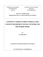
are referred to as neurons. The neurons are connected to one another with the use of axons and dendrites, and the connecting regions between axons and dendrites are referred to
as synapses. These connections are illustrated in Figure 1.1(a). The strengths of synaptic
connections often change in response to external stimuli. This change is how learning takes
place in living organisms.
This biological mechanism is simulated in artificial neural networks, which contain computation units that are referred to as neurons. Throughout this book, we will use the term
“neural networks” to refer to artificial neural networks rather than biological ones. The
computational units are connected to one another through weights, which serve the same

w1
w2
w3

NEURON

AXON


w4
w5
DENDRITES WITH
SYNAPTIC WEIGHTS

(a) Biological neural network

(b) Artificial neural network

Figure 1.1: The synaptic connections between neurons. The image in (a) is from “The Brain:
Understanding Neurobiology Through the Study of Addiction [598].” Copyright c 2000 by
BSCS & Videodiscovery. All rights reserved. Used with permission.
© Springer International Publishing AG, part of Springer Nature 2018
C. C. Aggarwal, Neural Networks and Deep Learning,
1

1


2

CHAPTER 1. AN INTRODUCTION TO NEURAL NETWORKS

role as the strengths of synaptic connections in biological organisms. Each input to a neuron
is scaled with a weight, which affects the function computed at that unit. This architecture
is illustrated in Figure 1.1(b). An artificial neural network computes a function of the inputs
by propagating the computed values from the input neurons to the output neuron(s) and
using the weights as intermediate parameters. Learning occurs by changing the weights connecting the neurons. Just as external stimuli are needed for learning in biological organisms,
the external stimulus in artificial neural networks is provided by the training data containing examples of input-output pairs of the function to be learned. For example, the training

data might contain pixel representations of images (input) and their annotated labels (e.g.,
carrot, banana) as the output. These training data pairs are fed into the neural network by
using the input representations to make predictions about the output labels. The training
data provides feedback to the correctness of the weights in the neural network depending
on how well the predicted output (e.g., probability of carrot) for a particular input matches
the annotated output label in the training data. One can view the errors made by the neural
network in the computation of a function as a kind of unpleasant feedback in a biological
organism, leading to an adjustment in the synaptic strengths. Similarly, the weights between
neurons are adjusted in a neural network in response to prediction errors. The goal of changing the weights is to modify the computed function to make the predictions more correct in
future iterations. Therefore, the weights are changed carefully in a mathematically justified
way so as to reduce the error in computation on that example. By successively adjusting
the weights between neurons over many input-output pairs, the function computed by the
neural network is refined over time so that it provides more accurate predictions. Therefore,
if the neural network is trained with many different images of bananas, it will eventually
be able to properly recognize a banana in an image it has not seen before. This ability to
accurately compute functions of unseen inputs by training over a finite set of input-output
pairs is referred to as model generalization. The primary usefulness of all machine learning
models is gained from their ability to generalize their learning from seen training data to
unseen examples.
The biological comparison is often criticized as a very poor caricature of the workings
of the human brain; nevertheless, the principles of neuroscience have often been useful in
designing neural network architectures. A different view is that neural networks are built
as higher-level abstractions of the classical models that are commonly used in machine
learning. In fact, the most basic units of computation in the neural network are inspired by
traditional machine learning algorithms like least-squares regression and logistic regression.
Neural networks gain their power by putting together many such basic units, and learning
the weights of the different units jointly in order to minimize the prediction error. From
this point of view, a neural network can be viewed as a computational graph of elementary
units in which greater power is gained by connecting them in particular ways. When a
neural network is used in its most basic form, without hooking together multiple units, the

learning algorithms often reduce to classical machine learning models (see Chapter 2). The
real power of a neural model over classical methods is unleashed when these elementary
computational units are combined, and the weights of the elementary models are trained
using their dependencies on one another. By combining multiple units, one is increasing the
power of the model to learn more complicated functions of the data than are inherent in the
elementary models of basic machine learning. The way in which these units are combined
also plays a role in the power of the architecture, and requires some understanding and
insight from the analyst. Furthermore, sufficient training data is also required in order to
learn the larger number of weights in these expanded computational graphs.


1.1. INTRODUCTION

3

ACCURACY

DEEP LEARNING

CONVENTIONAL
MACHINE LEARNING

AMOUNT OF DATA

Figure 1.2: An illustrative comparison of the accuracy of a typical machine learning algorithm with that of a large neural network. Deep learners become more attractive than
conventional methods primarily when sufficient data/computational power is available. Recent years have seen an increase in data availability and computational power, which has
led to a “Cambrian explosion” in deep learning technology.

1.1.1


Humans Versus Computers: Stretching the Limits
of Artificial Intelligence

Humans and computers are inherently suited to different types of tasks. For example, computing the cube root of a large number is very easy for a computer, but it is extremely
difficult for humans. On the other hand, a task such as recognizing the objects in an image
is a simple matter for a human, but has traditionally been very difficult for an automated
learning algorithm. It is only in recent years that deep learning has shown an accuracy on
some of these tasks that exceeds that of a human. In fact, the recent results by deep learning
algorithms that surpass human performance [184] in (some narrow tasks on) image recognition would not have been considered likely by most computer vision experts as recently
as 10 years ago.
Many deep learning architectures that have shown such extraordinary performance are
not created by indiscriminately connecting computational units. The superior performance
of deep neural networks mirrors the fact that biological neural networks gain much of their
power from depth as well. Furthermore, biological networks are connected in ways we do not
fully understand. In the few cases that the biological structure is understood at some level,
significant breakthroughs have been achieved by designing artificial neural networks along
those lines. A classical example of this type of architecture is the use of the convolutional
neural network for image recognition. This architecture was inspired by Hubel and Wiesel’s
experiments [212] in 1959 on the organization of the neurons in the cat’s visual cortex. The
precursor to the convolutional neural network was the neocognitron [127], which was directly
based on these results.
The human neuronal connection structure has evolved over millions of years to optimize
survival-driven performance; survival is closely related to our ability to merge sensation and
intuition in a way that is currently not possible with machines. Biological neuroscience [232]
is a field that is still very much in its infancy, and only a limited amount is known about how
the brain truly works. Therefore, it is fair to suggest that the biologically inspired success
of convolutional neural networks might be replicated in other settings, as we learn more
about how the human brain works [176]. A key advantage of neural networks over traditional machine learning is that the former provides a higher-level abstraction of expressing
semantic insights about data domains by architectural design choices in the computational
graph. The second advantage is that neural networks provide a simple way to adjust the



4

CHAPTER 1. AN INTRODUCTION TO NEURAL NETWORKS

complexity of a model by adding or removing neurons from the architecture according to
the availability of training data or computational power. A large part of the recent success of neural networks is explained by the fact that the increased data availability and
computational power of modern computers has outgrown the limits of traditional machine
learning algorithms, which fail to take full advantage of what is now possible. This situation
is illustrated in Figure 1.2. The performance of traditional machine learning remains better
at times for smaller data sets because of more choices, greater ease of model interpretation,
and the tendency to hand-craft interpretable features that incorporate domain-specific insights. With limited data, the best of a very wide diversity of models in machine learning
will usually perform better than a single class of models (like neural networks). This is one
reason why the potential of neural networks was not realized in the early years.
The “big data” era has been enabled by the advances in data collection technology; virtually everything we do today, including purchasing an item, using the phone, or clicking on
a site, is collected and stored somewhere. Furthermore, the development of powerful Graphics Processor Units (GPUs) has enabled increasingly efficient processing on such large data
sets. These advances largely explain the recent success of deep learning using algorithms
that are only slightly adjusted from the versions that were available two decades back.
Furthermore, these recent adjustments to the algorithms have been enabled by increased
speed of computation, because reduced run-times enable efficient testing (and subsequent
algorithmic adjustment). If it requires a month to test an algorithm, at most twelve variations can be tested in an year on a single hardware platform. This situation has historically
constrained the intensive experimentation required for tweaking neural-network learning
algorithms. The rapid advances associated with the three pillars of improved data, computation, and experimentation have resulted in an increasingly optimistic outlook about the
future of deep learning. By the end of this century, it is expected that computers will have
the power to train neural networks with as many neurons as the human brain. Although
it is hard to predict what the true capabilities of artificial intelligence will be by then, our
experience with computer vision should prepare us to expect the unexpected.
Chapter Organization
This chapter is organized as follows. The next section introduces single-layer and multi-layer

networks. The different types of activation functions, output nodes, and loss functions are
discussed. The backpropagation algorithm is introduced in Section 1.3. Practical issues in
neural network training are discussed in Section 1.4. Some key points on how neural networks
gain their power with specific choices of activation functions are discussed in Section 1.5. The
common architectures used in neural network design are discussed in Section 1.6. Advanced
topics in deep learning are discussed in Section 1.7. Some notable benchmarks used by the
deep learning community are discussed in Section 1.8. A summary is provided in Section 1.9.

1.2

The Basic Architecture of Neural Networks

In this section, we will introduce single-layer and multi-layer neural networks. In the singlelayer network, a set of inputs is directly mapped to an output by using a generalized variation
of a linear function. This simple instantiation of a neural network is also referred to as the
perceptron. In multi-layer neural networks, the neurons are arranged in layered fashion, in
which the input and output layers are separated by a group of hidden layers. This layer-wise
architecture of the neural network is also referred to as a feed-forward network. This section
will discuss both single-layer and multi-layer networks.


1.2. THE BASIC ARCHITECTURE OF NEURAL NETWORKS

INPUT NODES

INPUT NODES

x1
x2
x3


x1
w1
w2
w3
w4

x4

5

∑

w1
w2

x2

OUTPUT NODE

y

w3

x3

∑

w4
x4


w5

OUTPUT NODE

y

w5

b

x5

x5

(a) Perceptron without bias

+1 BIAS NEURON

(b) Perceptron with bias

Figure 1.3: The basic architecture of the perceptron

1.2.1

Single Computational Layer: The Perceptron

The simplest neural network is referred to as the perceptron. This neural network contains
a single input layer and an output node. The basic architecture of the perceptron is shown
in Figure 1.3(a). Consider a situation where each training instance is of the form (X, y),
where each X = [x1 , . . . xd ] contains d feature variables, and y ∈ {−1, +1} contains the

observed value of the binary class variable. By “observed value” we refer to the fact that it
is given to us as a part of the training data, and our goal is to predict the class variable for
cases in which it is not observed. For example, in a credit-card fraud detection application,
the features might represent various properties of a set of credit card transactions (e.g.,
amount and frequency of transactions), and the class variable might represent whether or
not this set of transactions is fraudulent. Clearly, in this type of application, one would have
historical cases in which the class variable is observed, and other (current) cases in which
the class variable has not yet been observed but needs to be predicted.
The input layer contains d nodes that transmit the d features X = [x1 . . . xd ] with
edges of weight W = [w1 . . . wd ] to an output node. The input layer does not perform
d
any computation in its own right. The linear function W · X = i=1 wi xi is computed at
the output node. Subsequently, the sign of this real value is used in order to predict the
dependent variable of X. Therefore, the prediction yˆ is computed as follows:
d

yˆ = sign{W · X} = sign{

j=1

wj x j }

(1.1)

The sign function maps a real value to either +1 or −1, which is appropriate for binary
classification. Note the circumflex on top of the variable y to indicate that it is a predicted
value rather than an observed value. The error of the prediction is therefore E(X) = y − yˆ,
which is one of the values drawn from the set {−2, 0, +2}. In cases where the error value
E(X) is nonzero, the weights in the neural network need to be updated in the (negative)
direction of the error gradient. As we will see later, this process is similar to that used in

various types of linear models in machine learning. In spite of the similarity of the perceptron
with respect to traditional machine learning models, its interpretation as a computational
unit is very useful because it allows us to put together multiple units in order to create far
more powerful models than are available in traditional machine learning.