Many body quantum theory in condensed matter physics nodrm
Bạn đang xem bản rút gọn của tài liệu. Xem và tải ngay bản đầy đủ của tài liệu tại đây (3.66 MB, 458 trang )
Many-body Quantum Theory in
Condensed Matter Physics
Many-body Quantum Theory
in Condensed Matter Physics
an introduction
H E N R I K B RU U S
Department of Physics
Technical University of Denmark
and
K A R S T E N F L E N S B E RG
Niels Bohr Institute,
University of Copenhagen
Copenhagen, 14 July 2004
Corrected version: 14 January 2016
1
Great Clarendon Street, Oxford OX2 6DP
Oxford University Press is a department of the University of Oxford.
It furthers the University’s objective of excellence in research, scholarship,
and education by publishing worldwide in
Oxford New York
Auckland Cape Town Dar es Salaam Hong Kong Karachi
Kuala Lumpur Madrid Melbourne Mexico City Nairobi
New Delhi Shanghai Taipei Toronto
With offices in
Argentina Austria Brazil Chile Czech Republic France Greece
Guatemala Hungary Italy Japan South Korea Poland Portugal
Singapore Switzerland Thailand Turkey Ukraine Vietnam
Oxford is a registered trade mark of Oxford University Press
in the UK and in certain other countries
Published in the United States
by Oxford University Press Inc., New York
© Oxford University Press 2004
The moral rights of the author have been asserted
Database right Oxford University Press (maker)
First published 2004
Reprinted 2005, 2006, 2007 (twice), 2009 (twice), 2010, 2011,
2012 (twice), 2013, 2015, 2016 (with corrections)
All rights reserved. No part of this publication may be reproduced,
stored in a retrieval system, or transmitted, in any form or by any means,
without the prior permission in writing of Oxford University Press,
or as expressly permitted by law, or under terms agreed with the appropriate
reprographics rights organization. Enquiries concerning reproduction
outside the scope of the above should be sent to the Rights Department,
Oxford University Press, at the address above.
You must not circulate this book in any other binding or cover
and you must impose this same condition on any acquirer.
A catalogue record for this title is available from the British Library
Library of Congress Cataloging in Publication Data
(Data available)
ISBN 978-0-19-856633-5 (Hbk)
14
Printed in Great Britain
by CPI Group (UK) Ltd, Croydon, CR0 4YY
PREFACE
This introduction to many-body quantum theory in condensed matter physics has
emerged from a set of lecture notes used in our courses Many-particle Physics I and
II for graduate and advanced undergraduate students at the Niels Bohr Institute,
University of Copenhagen, held six times between 1999 and 2004. The notes have also
been used twice in the course Transport in Nanostructures taught at the Technical
University of Denmark. The courses have been followed by students of both theoretical
and experimental physics and it is our experience that both groups have benefited
from the notes. The theory students gained a good background for further studies,
while the experimental students obtained a familiarity with theoretical concepts they
encounter in research papers.
We have gone through the trouble of writing this textbook, because we felt the
pedagogical need for putting an emphasis on the physical contents and applications of
the machinery of quantum field theory without loosing mathematical rigor. We hope
we have succeeded, at least to some extent, in reaching this goal.
Since our main purpose is to provide a pedagogical introduction, and not to present
a review of the physical examples presented, we do not give comprehensive references
to these topics. Instead, we refer the reader to the review papers and topical books
mentioned in the text and in the bibliography.
We would like to thank our ever enthusiastic students for their valuable help
throughout the years improving the notes preceding this book.
Copenhagen, July 2004.
Karsten Flensberg
Ørsted Laboratory
Niels Bohr Institute
University of Copenhagen
Henrik Bruus
MIC – Department of
Micro and Nanotechnology
Technical University of Denmark
Preface to corrected edition January 2016.
The book has been corrected for an, unfortunately, rather large number of misprints. We would like to thank all the colleagues and readers who have sent corrections
to us and in particular the many students and the teachers of the courses Condensed
Matter Theory I at University of Copenhagen and Transport in nanostructures at
the Technical University of Denmark for helping in locating the misprints. We have
not made major changes to the book other than Section 10.5 has been rewritten
somewhat.
Karsten Flensberg
Niels Bohr Institute
University of Copenhagen
Henrik Bruus
Department of Physics
Technical University of Denmark
v
CONTENTS
List of symbols
xiv
1
First and second quantization
1.1 First quantization, single-particle systems
1.2 First quantization, many-particle systems
1.2.1 Permutation symmetry and indistinguishability
1.2.2 The single-particle states as basis states
1.2.3 Operators in first quantization
1.3 Second quantization, basic concepts
1.3.1 The occupation number representation
1.3.2 The boson creation and annihilation operators
1.3.3 The fermion creation and annihilation operators
1.3.4 The general form for second quantization operators
1.3.5 Change of basis in second quantization
1.3.6 Quantum field operators and their Fourier transforms
1.4 Second quantization, specific operators
1.4.1 The harmonic oscillator in second quantization
1.4.2 The electromagnetic field in second quantization
1.4.3 Operators for kinetic energy, spin, density and current
1.4.4 The Coulomb interaction in second quantization
1.4.5 Basis states for systems with different particles
1.5 Second quantization and statistical mechanics
1.5.1 The distribution function for non-interacting fermions
1.5.2 The distribution function for non-interacting bosons
1.6 Summary and outlook
1
2
4
5
6
8
10
10
10
13
14
16
17
18
18
19
21
23
25
26
29
29
30
2
The electron gas
2.1 The non-interacting electron gas
2.1.1 Bloch theory of electrons in a static ion lattice
2.1.2 Non-interacting electrons in the jellium model
2.1.3 Non-interacting electrons at finite temperature
2.2 Electron interactions in perturbation theory
2.2.1 Electron interactions in 1st -order perturbation theory
2.2.2 Electron interactions in 2nd -order perturbation theory
2.3 Electron gases in 3, 2, 1 and 0 dimensions
2.3.1 3D electron gases: metals and semiconductors
2.3.2 2D electron gases: GaAs/GaAlAs heterostructures
2.3.3 1D electron gases: carbon nanotubes
2.3.4 0D electron gases: quantum dots
2.4 Summary and outlook
32
33
33
36
39
40
42
44
45
45
47
49
50
51
vii
viii
CONTENTS
3
Phonons; coupling to electrons
3.1 Jellium oscillations and Einstein phonons
3.2 Electron–phonon interaction and the sound velocity
3.3 Lattice vibrations and phonons in 1D
3.4 Acoustical and optical phonons in 3D
3.5 The specific heat of solids in the Debye model
3.6 Electron–phonon interaction in the lattice model
3.7 Electron–phonon interaction in the jellium model
3.8 Summary and outlook
52
52
53
54
57
59
61
64
65
4
Mean-field theory
4.1 Basic concepts of mean-field theory
4.2 The art of mean-field theory
4.3 Hartree–Fock approximation
4.3.1 H–F approximation for the homogenous electron gas
4.4 Broken symmetry
4.5 Ferromagnetism
4.5.1 The Heisenberg model of ionic ferromagnets
4.5.2 The Stoner model of metallic ferromagnets
4.6 Summary and outlook
66
66
69
70
71
72
74
74
76
78
5
Time dependence in quantum theory
5.1 The Schrăodinger picture
5.2 The Heisenberg picture
5.3 The interaction picture
5.4 Time-evolution in linear response
5.5 Time-dependent creation and annihilation operators
5.6 Fermi’s golden rule
5.7 The T -matrix and the generalized Fermi’s golden rule
5.8 Fourier transforms of advanced and retarded functions
5.9 Summary and outlook
80
80
81
81
84
84
86
87
88
90
6
Linear response theory
6.1 The general Kubo formula
6.1.1 Kubo formula in the frequency domain
6.2 Kubo formula for conductivity
6.3 Kubo formula for conductance
6.4 Kubo formula for the dielectric function
6.4.1 Dielectric function for translation-invariant system
6.4.2 Relation between dielectric function and conductivity
6.5 Summary and outlook
92
92
94
95
97
98
100
100
101
CONTENTS
ix
7
Transport in mesoscopic systems
7.1 The S-matrix and scattering states
7.1.1 Definition of the S-matrix
7.1.2 Definition of the scattering states
7.1.3 Unitarity of the S-matrix
7.1.4 Time-reversal symmetry
7.2 Conductance and transmission coefficients
7.2.1 The Landauer formula, heuristic derivation
7.2.2 The Landauer formula, linear response derivation
7.2.3 LandauerBă
uttiker formalism for multiprobe systems
7.3 Electron wave guides
7.3.1 Quantum point contact and conductance quantization
7.3.2 The Aharonov–Bohm effect
7.4 Summary and outlook
102
103
103
106
106
107
108
109
111
112
113
113
117
118
8
Green’s functions
8.1 Classical Greens functions
8.2 Greens function for the one-particle Schrăodinger equation
8.2.1 Example: from the S-matrix to the Green’s function
8.3 Single-particle Green’s functions of many-body systems
8.3.1 Green’s function of translation-invariant systems
8.3.2 Green’s function of free electrons
8.3.3 The Lehmann representation
8.3.4 The spectral function
8.3.5 Broadening of the spectral function
8.4 Measuring the single-particle spectral function
8.4.1 Tunneling spectroscopy
8.5 Two-particle correlation functions of many-body systems
8.6 Summary and outlook
120
120
120
123
124
125
125
127
129
130
131
132
135
138
9
Equation of motion theory
9.1 The single-particle Green’s function
9.1.1 Non-interacting particles
9.2 Single level coupled to a continuum
9.3 Anderson’s model for magnetic impurities
9.3.1 The equation of motion for the Anderson model
9.3.2 Mean-field approximation for the Anderson model
9.4 The two-particle correlation function
9.4.1 The random phase approximation
9.5 Summary and outlook
139
139
141
141
142
144
145
148
148
150
10 Transport in interacting mesoscopic systems
10.1 Model Hamiltonians
10.2 Sequential tunneling: the Coulomb blockade regime
10.2.1 Coulomb blockade for a metallic dot
10.2.2 Coulomb blockade for a quantum dot
151
151
153
154
157
x
CONTENTS
10.3 Coherent many-body transport phenomena
10.3.1 Cotunneling
10.3.2 Inelastic cotunneling for a metallic dot
10.3.3 Elastic cotunneling for a quantum dot
10.4 The conductance for Anderson-type models
10.4.1 The conductance in linear response
10.4.2 Calculation of Coulomb blockade peaks
10.5 The Kondo effect in quantum dots
10.5.1 From the Anderson model to the Kondo model
10.5.2 Comparing Kondo effect in metals and quantum dots
(2)
10.5.3 Kondo-model conductance to second order in HS
(2)
10.5.4 Kondo-model conductance to third order in HS
10.5.5 Origin of the logarithmic divergence
10.5.6 The Kondo problem beyond perturbation theory
10.6 Summary and outlook
158
158
159
160
161
162
165
168
168
173
173
174
179
181
182
11 Imaginary-time Green’s functions
11.1 Definitions of Matsubara Green’s functions
11.1.1 Fourier transform of Matsubara Green’s functions
11.2 Connection between Matsubara and retarded functions
11.2.1 Advanced functions
11.3 Single-particle Matsubara Green’s function
11.3.1 Matsubara Green’s function, non-interacting particles
11.4 Evaluation of Matsubara sums
11.4.1 Summations over functions with simple poles
11.4.2 Summations over functions with known branch cuts
11.5 Equation of motion
11.6 Wick’s theorem
11.7 Example: polarizability of free electrons
11.8 Summary and outlook
184
187
188
189
191
192
192
193
194
196
197
198
201
202
12 Feynman diagrams and external potentials
12.1 Non-interacting particles in external potentials
12.2 Elastic scattering and Matsubara frequencies
12.3 Random impurities in disordered metals
12.3.1 Feynman diagrams for the impurity scattering
12.4 Impurity self-average
12.5 Self-energy for impurity scattered electrons
12.5.1 Lowest-order approximation
12.5.2 First-order Born approximation
12.5.3 The full Born approximation
12.5.4 Self-consistent full Born approximation and beyond
12.6 Summary and outlook
204
204
206
208
209
211
216
217
217
220
222
224
CONTENTS
13 Feynman diagrams and pair interactions
13.1 The perturbation series for G
13.2 The Feynman rules for pair interactions
13.2.1 Feynman rules for the denominator of G(b, a)
13.2.2 Feynman rules for the numerator of G(b, a)
13.2.3 The cancellation of disconnected Feynman diagrams
13.3 Self-energy and Dyson’s equation
13.4 The Feynman rules in Fourier space
13.5 Examples of how to evaluate Feynman diagrams
13.5.1 The Hartree self-energy diagram
13.5.2 The Fock self-energy diagram
13.5.3 The pair-bubble self-energy diagram
13.6 Cancellation of disconnected diagrams, general case
13.7 Feynman diagrams for the Kondo model
13.7.1 Kondo model self-energy, second order in J
13.7.2 Kondo model self-energy, third order in J
13.8 Summary and outlook
14 The interacting electron gas
14.1 The self-energy in the random phase approximation
14.1.1 The density dependence of self-energy diagrams
14.1.2 The divergence number of self-energy diagrams
14.1.3 RPA resummation of the self-energy
14.2 The renormalized Coulomb interaction in RPA
14.2.1 Calculation of the pair-bubble
14.2.2 The electron-hole pair interpretation of RPA
14.3 The groundstate energy of the electron gas
14.4 The dielectric function and screening
14.5 Plasma oscillations and Landau damping
14.5.1 Plasma oscillations and plasmons
14.5.2 Landau damping
14.6 Summary and outlook
15 Fermi liquid theory
15.1 Adiabatic continuity
15.1.1 Example: one-dimensional well
15.1.2 The quasiparticle concept and conserved quantities
15.2 Semi-classical treatment of screening and plasmons
15.2.1 Static screening
15.2.2 Dynamical screening
15.3 Semi-classical transport equation
15.3.1 Finite lifetime of the quasiparticles
15.4 Microscopic basis of the Fermi liquid theory
15.4.1 Renormalizationofthesingle-particleGreen’s function
15.4.2 Imaginary part of the single-particle Green’s function
15.4.3 Mass renormalization?
15.5 Summary and outlook
xi
226
227
228
229
230
231
233
233
236
236
237
238
239
241
243
244
245
246
246
247
248
248
250
251
253
253
256
260
262
263
264
266
266
267
268
269
270
271
272
276
278
278
280
283
283
xii
CONTENTS
16 Impurity scattering and conductivity
16.1 Vertex corrections and dressed Green’s functions
16.2 The conductivity in terms of a general vertex function
16.3 The conductivity in the first Born approximation
16.4 Conductivity from Born scattering with interactions
16.5 The weak localization correction to the conductivity
16.6 Disordered mesoscopic systems
16.6.1 Statistics of quantum conductance,
random matrix theory
16.6.2 Weak localization in mesoscopic systems
16.6.3 Universal conductance fluctuations
16.7 Summary and outlook
17 Green’s functions and phonons
17.1 The Green’s function for free phonons
17.2 Electron–phonon interaction and Feynman diagrams
17.3 Combining Coulomb and electron–phonon interactions
17.3.1 Migdal’s theorem
17.3.2 Jellium phonons and the effective
electron–electron interaction
17.4 Phonon renormalization by electron screening in RPA
17.5 The Cooper instability and Feynman diagrams
17.6 Summary and outlook
18 Superconductivity
18.1 The Cooper instability
18.2 The BCS groundstate
18.3 Microscopic BCS theory
18.4 BCS theory with Matsubara Green’s functions
18.4.1 Self-consistent determination of
the BCS order parameter ∆k
18.4.2 Determination of the critical temperature Tc
18.4.3 Determination of BCS quasiparticle density of states
18.5 The Nambu formalism of the BCS theory
18.5.1 Spinors and Green’s functions in Nambu formalism
18.5.2 The Meissner effect and the London equation
18.5.3 Zero paramagnetic current response in BCS theory
18.6 Gauge symmetry breaking and zero resistivity
18.6.1 Gauge transformations
18.6.2 Broken gauge symmetry and dissipationless current
18.7 The Josephson effect
18.8 Summary and outlook
285
286
291
293
296
298
308
308
309
310
312
313
313
314
316
317
318
319
322
324
325
325
327
329
331
332
333
334
335
335
336
337
341
341
342
343
346
CONTENTS
xiii
19 1D electron gases and Luttinger liquids
19.1 What is a Luttinger liquid?
19.2 Experimental realizations of Luttinger liquid physics
19.2.1 Example: Carbon Nanotubes
19.2.2 Example: semiconductor wires
19.2.3 Example: quasi 1D materials
19.2.4 Example: Edge states in fractional quantum Hall effect
19.3 A first look at the theory of interacting electrons in 1D
19.3.1 The “quasiparticles” in 1D
19.3.2 The lifetime of the “quasiparticles” in 1D
19.4 The spinless Luttinger–Tomonaga model
19.4.1 The Luttinger–Tomonaga model Hamiltonian
19.4.2 Inter-branch interaction
19.4.3 Intra-branch interaction and charge conservation
19.4.4 Umklapp processes in the half-filled band case
19.5 Bosonization of the Tomonaga model Hamiltonian
19.5.1 Derivation of the bosonized Hamiltonian
19.5.2 Diagonalization of the bosonized Hamiltonian
19.5.3 Real space representation
19.6 Electron operators in bosonized form
19.7 Green’s functions
19.8 Measuring local density of states by tunneling
19.9 Luttinger liquid with spin
19.10 Summary and outlook
347
347
348
348
348
348
348
348
350
351
352
352
354
355
356
357
357
360
360
363
368
369
373
374
A Fourier transformations
A.1 Continuous functions in a finite region
A.2 Continuous functions in an infinite region
A.3 Time and frequency Fourier transforms
A.4 Some useful rules
A.5 Translation-invariant systems
376
376
377
377
377
378
Exercises
380
Bibliography
423
Index
426
LIST OF SYMBOLS
Symbol
Meaning
Definition
ˆ
♥
operator ♥ in the interaction picture
time derivative of ♥
Dirac ket notation for a quantum state ν
Dirac bra notation for an adjoint quantum state ν
vacuum state
Section 5.3
Section 1.1
Section 1.1
Section 1.3
a
a†
aν , a†ν
a±
n
a0
A(r, t)
A(ν, ω)
A(r, ω), A(k, ω)
A0 (r, ω), A0 (k, ω)
A, A†
annihilation operator for particle (fermion or boson)
creation operator for particle (fermion or boson)
annihilation/creation operators (state ν)
amplitudes of wavefunctions to the left
Bohr radius
electromagnetic vector potential
spectral function in frequency domain (state ν)
spectral function (real space, Fourier space)
spectral function for free particles
phonon annihilation and creation operator
Section 1.3
Section 1.3
Section 1.3
Section 7.1
Eq. (2.36)
Section 1.4.2
Section 8.3.4
Section 8.3.4
Section 8.3.4
Section 17.1
b
β
b†
b±
n
B
annihilation operator for particle (boson, phonon)
inverse temperature
creation operator for particle (boson, phonon)
amplitudes of wavefunctions to the right
magnetic field
Section 1.3
Eq. (1.113)
Section 1.3
Section 7.1
c
c†
cν , c†ν
R
CAB
(t, t )
A
CAB (t, t )
R
CII
(ω)
CAB
C(Q, ikn , ikn + iqn )
C R (Q, ε, ε)
CVion
annihilation operator for particle (fermion, electron)
creation operator for particle (fermion, electron)
annihilation/creation operators (state ν)
retarded correlation function between A and B (time)
advanced correlation function between A and B (time)
retarded current–current correlation function (frequency)
Matsubara correlation function
Cooperon in the Matsubara domain
Cooperon in the real time domain
specific heat for ions (constant volume)
Section
Section
Section
Section
Section
Section
Section
Section
Section
Section
˙
♥
|ν
ν|
|0
xiv
1.3
1.3
1.3
6.1
11.2.1
6.3
11.1
16.5
16.5
3.5
LIST OF SYMBOLS
d( )
D
DR (rt, rt )
DR (q, ω)
D(rτ, rτ )
D(q, iqn )
DR (νt, ν t )
Dαβ (r)
δ(r)
δij
∆k
density of states (including spin degeneracy)
band width
retarded phonon propagator
retarded phonon propagator (Fourier space)
Matsubara phonon propagator
Matsubara phonon propagator (Fourier space)
retarded many particle Green’s function
phonon dynamical matrix
Dirac delta function
Kronecker’s delta function
superconducting orderparameter
e
e20
E(r, t)
E
E (1)
E (2)
E0
Ek
ε
elementary charge
electron interaction strength
electric field
total energy of the electron gas
interaction energy, first-order perturbation
interaction energy, second-order perturbation
Rydberg energy
dispersion relation for BCS quasiparticles
energy variable
the dielectric constant of vacuum
dispersion relation
energy of quantum state ν
Fermi energy
phonon polarization vector
dielectric function in real space
dielectric function in Fourier space
dielectric function in Fourier space
Levi–Civita symbol
0
εk
εν
εF
kλ
ε(rt, rt )
ε(k, ω)
ε(k, ω)
ijk
xv
Eq. (2.31)
Chapter 17
Chapter 17
Chapter 17
Chapter 17
Eq. (9.9b)
Section 3.4)
Eq. (1.12)
Eq. (1.10)
Eq. (18.11)
Eq. (1.100a)
Chapter 2
Section 2.2.1
Section 2.2.2
Eq. (2.36)
Eq. (18.14)
Chapter 2
Eq. (3.20)
Section 6.4
Section 6.4
Section 6.4
Eq. (1.11)
F
F
|FS
φ(x)
φ(r, t)
φext
φind
φ, φ˜
±
φ±
LnE , φRnE
free energy
Anomalous Green’s function
the filled Fermi sea N –particle quantum state
displacement field operator
electric potential
external electric potential
induced electric potential
wavefunctions with different normalizations
wavefunctions in the left and right leads
Section 1.5
Eq. (18.18)
Eq. (2.22)
Eq. (19.49)
Section 6.4
Section 6.4
Section 6.4
Eq. (7.4)
Section 7.1
gqλ
gq
G
electron–phonon coupling constant (lattice model)
electron–phonon coupling constant (jellium model)
conductance
Eq. (3.38)
Eq. (3.42)
Section 6.3
xvi
LIST OF SYMBOLS
G<
0 (rt, r t )
G>
0 (rt, r t )
GA
0 (rt, r t )
GR
0 (rt, r t )
GR
0 (k, ω)
G< (rt, r t )
G> (rt, r t )
GA (rt, r t )
GR (rt, r t )
GR (k, ω)
GR (k, ω)
GR (νt, ν t )
¯
G(k,
τ)
G(rστ, r σ τ )
G(ντ, ν τ )
G(1, 1 )
˜ k
˜)
G(k,
G0 (rστ, r σ τ )
G0 (ντ, ν τ )
G0 (k, ikn )
G0 (ν, ikn )
(n)
G0
G(k, ikn )
G(ν, ikn )
γ, γ RA
Γ
˜ k
˜ + q˜)
Γx (k,
Γ0,x
Γf i
free lesser Green’s function
free grater Green’s function
free advanced Green’s function
free retarded Green’s function
free retarded Green’s function (Fourier space)
lesser Green’s function
greater Green’s function
advanced Green’s function
retarded Green’s function (real space)
retarded Green’s function in Fourier space
retarded Green’s function (Fourier space)
retarded single–particle Green’s function ({ν} basis)
Nambu Green’s function
Matsubara Green’s function (real space)
Matsubara Green’s function ({ν} basis)
Matsubara Green’s function (real space four–vectors)
Matsubara Green’s function (four–momentum notation)
Matsubara Green’s function (real space, free particles)
Matsubara Green’s function ({ν} basis, free particles)
Matsubara Green’s function (Fourier space, free particles)
Matsubara Green’s function (free particles )
n–particle Green’s function (free particles)
Matsubara Green’s function (Fourier space)
Matsubara Green’s function ({ν} basis, frequency domain)
scalar vertex function
imaginary part of self–energy
vertex function (x–component, four vector notation)
free (undressed) vertex function
transition rate
Eq. (16.21b)
Eq. (16.20)
Eq. (5.34)
H
H0
H
Hext
Hint
Hph
HT
η
Planck’s constant (h/2π), → 1 in Chap. 5 and onwards
a general Hamiltonian
unperturbed part of an Hamiltonian
perturbative part of an Hamiltonian
external potential part of an Hamiltonian
interaction part of an Hamiltonian
phonon part of an Hamiltonian
tunneling Hamiltonian
positive infinitisimal
Eq. (8.65)
Section 5.8
I
Ie
current operator (particle current)
electrical current (charge current)
Section 6.3
Section 6.3
Section 8.3.1
Section 8.3.1
Section 8.3.1
Section 8.3.1
Section 8.3.1
Section 8.3
Section 8.3
Section 8.3
Section 8.3
Section 8.3
Section 8.3.1
Eq. (8.34)
Eq. (18.44)
Section 11.3
Section 11.3
Section 12.1
Section 13.4
Section 11.3.1
Section 11.3.1
Section 11.3
Section 11.3
Section 11.6
Section 11.3
Section 11.3
Section 16.3
LIST OF SYMBOLS
xvii
Jσ (r)
Jσ∆ (r)
JσA (r)
Jσ (q)
Je (r, t)
Jij
Jαβ
current density operator
current density operator, paramagnetic term
current density operator, diamagnetic term
current density operator (momentum space)
electric current density operator
interaction strength in the Heisenberg model
interaction strength in the Kondo model
Eq. (1.98a)
Eq. (1.98a)
Eq. (1.98a)
Eq. (1.98a)
Section 6.2
Section 4.5.1
Eq. (10.91a)
kB
kn
kF
k
Boltzmann’s constant
Matsubara frequency (fermions)
Fermi wave number
general momentum or wave vector variable
Eq. (11.42)
Chapter 2
,
L
λF
Λirr
mean free path or scattering length
vk τ0 mean free path (first Born approximation)
phase breaking mean free path
normalization length or system size in 1D
Fermi wave length
irreducible four–point function
m
m∗
µ
µ
mass (electrons and general particles)
effective interaction renormalized mass
chemical potential
general quantum number label
n
nF (ε)
nB (ε)
nimp
N
Nimp
ν
particle density
Fermi–Dirac distribution function
Bose–Einstein distribution function
impurity density
number of particles
number of impurities
general quantum number label
ω
ωq
ωn
Ω
frequency variable
phonon dispersion relation
Matsubara frequency (boson)
thermodynamic potential
p
pn
P (x)
P
ΠR
αβ (rt, r t )
ΠR
αβ (q, ω)
Παβ (q, iωn )
Π0 (q, iqn )
general momentum or wave number variable
Matsubara frequency (fermion)
momentum field operator
principle part
retarded current–current correlation function
retarded current–current correlation function
Matsubara current–current correlation function
free pair–bubble diagram
k
0
φ
Chapter 12
Chapter 7
Eq. (2.23)
Eq. (16.18)
Section 15.4.1
Eq. (1.120)
Section 1.5.1
Section 1.5.2
Eq. (11.28)
Section 1.5
Eq. (11.28)
Eq. (19.50)
Eq. (6.25)
Chapter 16
Eq. (13.37)
xviii
LIST OF SYMBOLS
q
qn
general momentum variable
Matsubara frequency (bosons)
Eq. (11.28)
r
r
r
rs
ρ
ρ0
ρσ (r)
ρσ (q)
ρL , ρ R
general space variable
reflection matrix coming from left
reflection matrix coming from right
electron gas density parameter
density matrix
unperturbed density matrix
particle density operator (real space)
particle density operator (momentum space)
left and right mover density operators
Section 7.1
Section 7.1
Eq. (2.37)
Section 1.5
Eq. (6.3b)
Eq. (1.94)
Eq. (1.94)
Eq. (19.20)
S
Sx
σ
σαβ (rt, r t )
ΣR (q, ω)
Σ(q, ikn )
Σk
Σ1BA
k
ΣFBA
k
ΣSCBA
k
Σ(l, j)
Σσ (k, ikn )
ΣF
σ (k, ikn )
ΣH
σ (k, ikn )
ΣP
σ (k, ikn )
ΣRPA
(k, ikn )
σ
scattering matrix
spin operator
general spin index
conductivity tensor
retarded self–energy (Fourier space)
Matsubara self–energy
impurity scattering self–energy
first Born approximation
full Born approximation
self–consistent Born approximation
general electron self–energy
general electron self–energy
Fock self–energy
Hartree self–energy
pair–bubble self–energy
RPA electron self–energy
t
t
t
T
T
T
τ
i
τσσ
tr
τ
τ0 , τk
general time variable
tranmission matrix coming from left
transmission matrix coming from right
temperature
kinetic energy
T–matrix
general imaginary time variable
Pauli’s spin matrixes
transport scattering time
life–time in the first Born approximation
Section 5.7
Chapter 11
Eq. (1.91)
Eq. (15.38)
Section 12.5.2
uj
u(R0 )
uk
U
ˆ (t, t )
U
ˆ
U (τ, τ )
ion displacement (1D)
ion displacement (3D)
BCS coherence factor
general unitary matrix
real time–evolution operator, interaction picture
imaginary time–evolution operator, interaction picture
Eq. (3.8)
Section 3.4
Section 18.3
Section 16.6
Section 5.3
Eq. (11.12)
Section 7.1
Eq. (1.92b)
Section 6.2
Section
Section
Section
Section
12.5
12.5.1
12.5.3
12.5.4
Section 13.5
Section 13.5
Section 13.5
Eq. (14.11)
Section 7.1
Section 7.1
LIST OF SYMBOLS
xix
vk
V (r), V (q)
V (r), V (q)
Veff
V
BCS coherence factor
general single impurity potential
Coulomb interaction
combined Coulomb and phonon–mediated interaction
normalization volume
Section 18.3
Eq. (12.1)
Eq. (1.100a)
Section 14.2
W
W (r), W (q)
W RPA
pair interaction Hamiltonian
pair interaction
RPA–screened Coulomb interaction
Chapter 13
Chapter 13
Section 14.2
ξk
ξν
χ(q, iqn )
χRPA (q, iqn )
χirr (q, iqn )
χ0 (q, iqn )
χR (rt, r t )
χR (q, ω)
χn (y)
εk − µ
εν − µ
Matsubara charge–charge correlation function
RPA Matsubara charge–charge correlation function
irreducible Matsubara charge–charge correlation function
free Matsubara charge–charge correlation function
retarded charge–charge correlation function
retarded charge–charge correlation function (Fourier)
transverse wavefunction
Section 14.4
Section 14.4
Section 14.4
Section 14.4
Eq. (6.37b)
Eq. (8.81)
Section 7.1
ψν (r)
±
ψnE
ψ(r1 , r2 , . . . , rn )
Ψσ (r)
Ψ†σ (r)
single–particle wave function, quantum number ν
single–particle scattering states
n–particle wave function (first quantization)
quantum field annihilation operator
quantum field creation operator
Section
Section
Section
Section
Section
θ(x)
Heaviside’s step function
Eq. (1.13)
1.1
7.1
1.1
1.3.6
1.3.6
1
FIRST AND SECOND QUANTIZATION
Quantum theory is the most complete microscopic theory we have today describing the
physics of energy and matter. It has successfully been applied to explain phenomena
ranging over many orders of magnitude, from the study of elementary particles on
the sub-nucleonic scale to the study of neutron stars and other astrophysical objects
on the cosmological scale. Only the inclusion of gravitation stands out as an unsolved
problem in fundamental quantum theory.
Historically, quantum physics first dealt only with the quantization of the motion
of particles, leaving the electromagnetic field classical, hence the name quantum mechanics. Later also the electromagnetic field was quantized, and even the particles
themselves became represented by quantized fields, resulting in the development of
quantum electrodynamics (QED) and quantum field theory (QFT) in general. By convention, the original form of quantum mechanics is denoted first quantization, while
quantum field theory is formulated in the language of second quantization.
Regardless of the representation, be it first or second quantization, certain basic
concepts are always present in the formulation of quantum theory. The starting point
is the notion of quantum states and the observables of the system under consideration.
Quantum theory postulates that all quantum states are represented by state vectors in
a Hilbert space, and that all observables are represented by Hermitian operators acting
on that space. Parallel state vectors represent the same physical state, and therefore
one mostly deals with normalized state vectors. Any given Hermitian operator A has
a number of eigenstates |ψα that are left invariant by the action of the operator
up to a real scale factor α, i.e., A|ψα = α|ψα . The scale factors are denoted the
eigenvalues of the operator. It is a fundamental theorem of Hilbert space theory that
the set of all eigenvectors of any given Hermitian operator forms a complete basis
set of the Hilbert space. In general, the eigenstates |ψα and |φβ of two different
Hermitian operators A and B are not the same. By measurement of the type B the
quantum state can be prepared to be in an eigenstate |φβ of the operator B. This
state can also be expressed as a superposition of eigenstates |ψα of the operator A
as |φβ = α |ψα Cαβ . If one measures the dynamical variable associated with the
operator A in this state, one cannot in general predict the outcome with certainty.
It is only described in probabilistic terms. The probability of having any given |ψα
as the outcome is given as the absolute square |Cαβ |2 of the associated expansion
coefficient. This non-causal element of quantum theory is also known as the collapse
of the wavefunction. However, between collapse events the time evolution of quantum
states is perfectly deterministic. The time evolution of a state vector |ψ(t) is governed
by the central operator in quantum mechanics, the Hamiltonian H (the operator
associated with the total energy of the system), through Schrăodingers equation
1
2
FIRST AND SECOND QUANTIZATION
i ∂t ψ(t) = H ψ(t) .
(1.1)
Each state vector |ψ is associated with an adjoint state vector (|ψ )† ≡ ψ|. One
can form inner products, “bra(c)kets”, ψ|φ between adjoint “bra” states ψ| and
“ket” states |φ , and use standard geometrical terminology; e.g., the norm squared
of |ψ is given by ψ|ψ , and |ψ and |φ are said to be orthogonal if ψ|φ = 0.
If {|ψα } is an orthonormal basis of the Hilbert space, then the above-mentioned
expansion coefficient Cαβ is found by forming inner products: Cαβ = ψα |φβ . A
further connection between the direct and the adjoint Hilbert space is given by the
relation ψ|φ = φ|ψ ∗ , which also leads to the definition of adjoint operators. For
a given operator A the adjoint operator A† is defined by demanding ψ|A† |φ =
φ|A|ψ ∗ for any |ψ and |φ .
In this chapter, we will briefly review standard first quantization for one- and
many-particle systems. For more complete reviews the reader is referred to standard
textbooks by, for instance, Dirac (1989), Landau and Lifshitz (1977), and Merzbacher
(1970). Based on this we will introduce second quantization. This introduction, however, is not complete in all details, and we refer the interested reader to the textbooks
by Mahan (1990), Fetter and Walecka (1971), and Abrikosov et al. (1975).
1.1
First quantization, single-particle systems
For simplicity consider a non-relativistic particle, say an electron with charge −e,
moving in an external electromagnetic field described by the potentials ϕ(r, t) and
A(r, t). The corresponding Hamiltonian is
H=
1
2m
2
i
− e ϕ(r, t).
∇r + eA(r, t)
(1.2)
An eigenstate describing a free spin-up electron traveling inside a box of volume V
can be written as a product of a propagating plane wave and a spin-up spinor. Using
the Dirac notation the state ket can be written as |ψk,↑ = |k, ↑ , where one simply
lists the relevant quantum numbers in the ket. The state function (also denoted the
wave function) and the ket are related by
ψk,σ (r) = r|k, σ = √1V eik·r χσ
(free particle orbital),
(1.3)
i.e., by the inner product of the position bra r| with the state ket.
The plane wave representation |k, σ is not always a useful starting point for
calculations. For example in atomic physics, where electrons orbiting a point-like
positively charged nucleus are considered, the hydrogenic eigenstates |n, l, m, σ are
much more useful. Recall that
r|n, l, m, σ = Rnl (r)Yl,m (θ, φ)χσ
(hydrogen orbital),
(1.4)
where Rnl (r) is a radial Coulomb function with n − l nodes, while Yl,m (θ, φ) is a
spherical harmonic representing angular momentum l with a z component m.
A third example is an electron moving in a constant magnetic field B = B ez ,
which in the Landau gauge A = xB ey leads to the Landau eigenstates |n, ky , kz , σ ,
FIRST QUANTIZATION, SINGLE-PARTICLE SYSTEMS
(a)
(b)
3
(c)
Fig. 1.1. The probability density | r|ψν |2 in the xy plane for (a) any plane wave
ν = (kx , ky , kz , σ), (b) the hydrogen orbital ν = (4, 2, 0, σ), and (c) the Landau
orbital ν = (3, ky , 0, σ).
where n is an integer, ky (kz ) is the y (z) component of k, and σ the spin variable.
Recall that
1
r|n, ky , kz , σ = Hn (x/ − ky )e− 2 (x/
−ky )2
1
ei(ky y+kz z) χσ
(Landau orbital)
(1.5)
/eB is the magnetic length and Hn is the normalized Hermite polywhere =
nomial of order n associated with the harmonic oscillator potential induced by the
magnetic field. Examples of each of these three types of electron orbitals are shown
in Fig. 1.1.
In general a complete set of quantum numbers is denoted ν . The three examples
given above correspond to ν = (kx , ky , kz , σ), ν = (n, l, m, σ), and ν = (n, ky , kz , σ),
each yielding a state function of the form ψν (r) = r|ν . The completeness of a basis
state as well as the normalization of the state vectors plays a central role in quantum theory. Loosely speaking, the normalization condition means that with probability unity a particle in a given quantum state ψν (r) must be somewhere in space:
dr |ψν (r)|2 = 1, or in the Dirac notation: 1 = dr ν|r r|ν = ν| ( dr |r r|) |ν .
From this we conclude
√
Ly Lz
dr |r r| = 1.
(1.6)
Similarly, the completeness of a set of basis states ψν (r) means that if a particle is in
some state ψ(r) it must be found with probability unity within the orbitals of the basis
set: ν | ν|ψ |2 = 1. Again using the Dirac notation we find 1 = ν ψ|ν ν|ψ =
ψ| ( ν |ν ν|) |ψ , and we conclude
ν
|ν ν| = 1.
(1.7)
We shall often use the completeness relation (1.7). A simple example is the expansion
of a state function in a given basis: ψ(r) = r|ψ = r|1|ψ = r| ( ν |ν ν|) |ψ =
ν r|ν ν|ψ , which can be expressed as
ψ(r) =
ψν (r)
ν
dr ψν∗ (r )ψ(r )
or
r|ψ =
r|ν ν|ψ .
ν
(1.8)
4
FIRST AND SECOND QUANTIZATION
It should be noted that the quantum label ν can contain both discrete and continuous quantum numbers. In that case the symbol ν is to be interpreted as a combination of both summations and integrations. For example, in the case in Eq. (1.5)
with Landau orbitals in a box with side lengths Lx , Ly and Lz , we have
∞
=
ν
σ=↑,↓ n=0
∞
Ly
dky
−∞ 2π
∞
Lz
−∞ 2π
dkz .
(1.9)
In the mathematical formulation of quantum theory we shall often encounter the
following special functions:
• Kronecker’s delta-function δij for discrete variables,
δij =
• The Levi–Civita symbol
ijk
ijk
1, for i = j,
0, for i = j.
(1.10)
for discrete variables,
+1, if (ijk) is an even permutation of (123) or (xyz),
= −1, if (ijk) is an odd permutation of (123) or (xyz),
0, otherwise.
(1.11)
• Dirac’s delta-function δ(r) for continuous variables,
δ(r) = 0, for r = 0,
while
dr δ(r) = 1,
(1.12)
• and, finally, Heaviside’s step-function θ(x) for continuous variables,
θ(x) =
1.2
0, for x < 0,
1, for x > 0.
(1.13)
First quantization, many-particle systems
When turning to N-particle systems, i.e., systems containing N identical particles,
say, electrons, three more assumptions are added to the basic assumptions defining
quantum theory. The first assumption is the natural extension of the single-particle
state function ψ(r), which (neglecting the spin degree of freedom for the time being)
is a complex wave function in 3-dimensional space, to the N-particle state function
ψ(r1 , r2 , . . . , rN ), which is a complex function in the 3N-dimensional configuration
space. As for one particle, this N-particle state function is interpreted as a probability
amplitude such that its absolute square is related to a probability:
The probability for finding the N particles
N
N
in the 3N −dimensional volume j=1 drj
2
.
drj =
|ψ(r1 , r2 , . . . , rN )|
surrounding the point (r1 , r2 , . . . , rN ) in
j=1
the 3N −dimensional configuration space
(1.14)