Kayalar weinert1988 article errorboundsforthemethodofalter
Bạn đang xem bản rút gọn của tài liệu. Xem và tải ngay bản đầy đủ của tài liệu tại đây (600.12 KB, 17 trang )
Math. Control Signals Systems (1988) 1:43-59
Mathematics of Control,
Signals, and Systems
9 1988 Springer-Verlag New York Inc.
Error Bounds for the Method of Alternating Projections*
Selahattin K a y a l a r t and H o w a r d L. Weinertl"
Abstract. Given a collection of closed subspaces of a Hilbert space, the method
of alternating projections produces a sequencewhich converges to the orthogonal
projection onto the intersection of the subspaces. A large class of problems in
medical and geophysical image reconstruction can be solved using this method. A
sharp error bound will enable the user to estimate accurately the number of
iterations necessary to achieve a desired relative error. We obtain the sharpest
possible upper bound for the case of two subspaces, and the sharpest known upper
bound for more than two subspaces.
Key words. Alternating projections, Algebraic reconstruction technique, Error
bounds.
1. Introduction and Preliminaries
F o r k > 2 a n d i = 1, 2, . . . , k, let Hi be a closed subspace of a Hilbert space H, a n d
let P~ be the o r t h o g o n a l projection operator o n t o Hi. Define Hk= ~ as follows
H k : l = H k ca " " c~ H e ca H l 9
Let P be the o r t h o g o n a l projection operator o n t o Hk, 1.
N o w for a n y x ~ H consider the sequence {x~"~}~=1 defined by
X(1) = X
x ("§
= (Pk'"P2P1)x
0'~,
n =
I, 2 .....
This sequence converges strongly to P x , the o r t h o g o n a l projection of x o n t o the
intersection of all the subspaces; that is,
lim IJ(Pk'"P2P~)"x
-
Pxll
= O.
/l~gO
This iterative scheme, k n o w n as the m e t h o d of a l t e r n a t i n g p r o j e c t i o n s , ' w a s
established in the early 1930s by yon N e u m a n n for k = 2, b u t did n o t a p p e a r in
print until 1949-1950 I N 2 ] , [N3]. F o r k > 2, K a c z m a r z [ K 1 ] o b t a i n e d the result
in a m o r e specific setting, while H a l p e r i n [ H ] proved s t r o n g convergence lta the
* Date received:January 27, 1987. Date revised:April 21, 1987.This work was supported by the Office
of Naval Research under Contract N00014-85-K-0255.
"1"Department of Electrical and Computer Engineering, Johns Hopkins University, Baltimore,
Maryland 21218, U.S.A.
43
44
S. Kayalar and H. L. Weinert
general case stated above. Von Neumann's result was independently discovered by
Nakano I-N1] in 1940 and by Wiener [W-J in 1950.
The method of alternating projections has been applied in many areas, including
interpolation of stochastic processes IAA], [P], [S 1], reconstruction of bandlimited
functions [Y], solution of linear equations IT], and reconstruction of images in
medicine and geophysics [C], [I], IHS]. In these latter applications, the method is
known as the algebraic reconstruction technique (ART). Other applications are
mentioned by Deutsch [D1].
Our objective in this paper is to derive error bounds for the method of alternating
projections. A sharp bound will enable the user to estimate accurately the number
of iterations necessary to achieve a desired relative error. The relative error after n
iterations is given by
et"~(x) = II(Pk'"P2el)"x - extl/llxll.
We will obtain the sharpest possible upper bound on et"~(x) for k = 2, and the
sharpest known upper bound for k > 2, thus improving on the work of Aronszajn
[A-I, Youla [Y-J, Franchetti and Light I-FL], Deutsch [D2], and Hamaker and
Solmon I-HS].
Before getting started, we need to establish some facts about the angles between
subspaces. The concept of angles between subspaces of a Euclidean space is due to
Jordan [J]. The idea of a minimum angle between subspaces of a Hilbert space is
due to Friedrichs IF].
Definition 1. The minimum angle r
HI) between the subspaces H 2 and H1 is
the angle between 0 and re/2 whose cosine is given by
cos q~(H2, Hi) = sup{l(y, x)l: y e/-/2, x E Hi, IlYll < 1, tlxll < 1},
where ( . , 9) is the inner product in H.
If we remove the intersection from the two subspaces, we get a slightly different
definition.
Definition 2. The complementary angle r162 2, H1) between H 2 and Hx is
tpc(n2, Hi) = cP(n2 c~ n~.. 1, H1 n/-/21..1),
where H21:1 is the orthogonal complement of H2:1.
Note that if H2 c~ H i = {0}, then ~o(H2, H1) = ~(H2, HI). The angle introduced
by Friedrichs was actually the complementary angle.
The following lemma gives another relationship which will prove useful later.
L e m m a 1.
~(n2, H1 c~ H~..1) = opt(H2, H1).
Proof. For i = 1, 2, let Mi = Hi n//21.. 1. Since/-/2 = H2:1 + M2 is an orthogonal
direct sum decomposition of/-/2, any element y e/-/2 can be written uniquely as
Error Bounds for the Method of Alternating Projections
45
y = z + w where z ~ H2: t a n d w e M2. N o w
COS ~0(H2, M1)
= s u p { [ ( y , x)l: y ~ H2,
X
~ M1, IlYlt -< 1, Ilxll -< 1}
= s u p { l ( z + w, x)l: z ~ H2:1, w E M2, x ~ M1, IIz + wll < 1, Ilxll < 1}
-- sup{l(w, x ) t : w ~ M 2 ,
Ilwll -< 1, Ilxll -< 1}
x~M1,
= cos tp(M2, MI).
The third equality follows because (z, x ) = 0 and (z, w) = 0. The result of the
lemma then follows from Definition 2.
9
The next lemma is well k n o w n I F ] , [Y].
L e m m a 2.
cos tp(H2, H i ) = IIP2P, II =
~/IIP~P2Pxtl.
2. Fundamental Inequalities
The new inequalities given in the following lemmas are fundamental to our subsequent work.
Lemma 3.
L e t P 2 : 1 be the orthogonal projection operator o n t o H2:1 = H2 c~ H1,
and let L be any bounded operator on H. Then
[IP2PILII 2 <_ IIP1LII2c 2 + IIP2:tLII2s 2,
where c = cos (pc(H 2, Ha) and s 2 = 1 - c 2.
Proof. Let M1 = Ha c3 H~:t. Since H1 = H2:~ + M1 is an o r t h o g o n a l direct sum
decomposition of H 1, we have P1 = P2:1 + 1-11 and P2=IH1 = 0, where H 1 is the
o r t h o g o n a l projection o p e r a t o r o n t o Ma. Therefore, for every x E H,
IlelLxll 2 = IIP2:ILX + I-llLxll 2 = Ile2:lLxll 2 + [(rI1Lxl[ 2.
Similarly,
Ile2e, Lx[I 2 = ItP2P2:ILx + P21-l~Zxll 2 = IIe2:lLxl) 2 + IIP2HILxll 2.
We also k n o w that
Ile2Fla Zxll 2 = IIP2Hx rlx Lxll 2 < IIP2rlx II2 IlIIxZxll 2
= IIe2rI~ll2(llP1Zxll 2 -
IIe2:xZxll 2)
= c2(llP1Zxll 2 - IIP2:lZxl12).
Here we have used L e m m a s 1 and 2. Inserting this result into the previous equation
we get
IIP2PtLxll 2 < IlexLxll2c 2 + IIe2:tLxll2s 2,
and the desired result follows.
9
46
S. Kayalar and H. L. Weinert
F o r the next l e m m a let {Hj}T~ be a sequence of closed subspaces in H. N o w
define H,# to be
H i d = Hi ra Hj_l n " . n H#,
1 < j < i < m,
and let P , l be the o r t h o g o n a l projection o p e r a t o r onto H~,j.
L e m m a 4.
L e t c~:i = cos 9o(Hi..j, Hj_~), 2 .g j < i < m, and s2j = 1 - c~d. T h e n
IIP,,,"'P2P~II < f l p,,
l'l
where
~'i:i
2
(
i:3 ~ 2
c:+,i+~/c'~;,-t+'"+,=---'Ic+:2+\l.+_1,2]
p~=
~
Xi,2
2
11/'+"112 '
2
Y~:i = s~,is~:+-I ""si:l,
Fi..# = P i P i - l ' " P j ,
2 < j < i ~ m,
1 < j < i < m,
and ~a] = min {1, a}.
Proof. We will use the principle of strong induction [$2, p. 70] to p r o v e this lemma.
F o r m = 2, L e m m a 4 reduces to L e m m a 3 with L equal to identity. N o w assume
that the t h e o r e m is true for m = 3, 4 . . . . . i - 1. Then, for m = i, L e m m a 3 gives
[IPiPi-1 " "" P2P1 II2 -< IIPi-I "" "P2PI II2ci..i2 + IlPi,i-l Pi-2 " P2Pt II2si,.2
Applying L e m m a 3 to the second term on the right, we get
IIP.t-tPi-2""P2Pa II2 <
IIPi-2""P2PIII2c~.-~ + IIP~..~-2Ps-s'"P2P~ 112s~.-,.
C o n t i n u i n g in the same m a n n e r and collecting the resulting inequalities, we get
[IPiPi_a ... P2P~ I[2 ~ IJPi-x "" P2PI jl2c~i
+ IIPi-2
9
"'P2P~ II2v2
~ . . l : i U_2
i:i_l
+ IIP~-3 ""P2PI II2 Y..i-lc.+-z
2
2
+ IIPx II2 ' ~ .2i : 3 c i :22
+ l l P ~ x II2 x+.-22
N o w , we can use the hypothesis to bound the n o r m s on the right, which yields
ne,
ll <_ r?_,,,
c,,,_,
- + "'" + kr+_,:2J
l:2 +
()2
~
,.,-
lIP. j. II 2
]
Error Bounds for the Method of Alternating Projections
47
But we also k n o w that IIP~Pi-I""P~PIII ~ IIPi-1 ""P2Pt II ~ Fi-~:t. Therefore p2 =
min{1, a} = [a~ where a denotes the sum of terms in the brackets above. This proves
the lemma for m = i, and therefore it is true for all m.
9
The following observations a b o u t this lemma are important.
1. The factors Pi depend on the specific order of the o r t h o g o n a l projection
operators.
2. The factor Pi is the sum of i terms, and depends on the previous i - 1 factors.
3. In the last term of the factor p~, the n o r m of the orthogonal projection o p e r a t o r
is not replaced by one since
Ilei: 111 =
{01 /f Hi'l = {0}'
otherwise.
4. If Hm:l :~ {0}, then IIP~:~II = 1 and p~ = 1 for all i e [2, m]. Consequently,
IIPm'"P2P1 [I = I-I7'=1Pi = 1.
5. If Hi.., = {0} for some r e I2, i], then ci:j = 0 for all j e I-2, r-I. In this case p~
is the sum of i - r + 1 terms and depends only on i - r previous factors.
6. If Hi = H i - l , then IIPiPi-x'"e2ea [I = ItPi-x'"P2exII- In this case Pi = 1, since
ci:i = 0 and El: j = Y'i-1 ..j for allj e [2, i -- 1].
3. The Error Operator
Since SUpo~x~net")(X)= H(Pk"'P2Px)"--PI], the n o r m of the error o p e r a t o r
(Pk"" P2 PI)" - P is the sharpest possible upper b o u n d on the relative error. W e will
now prove two lemmas which will enable us to write the error o p e r a t o r as the
product of certain o r t h o g o n a l projection operators.
L e m m a 5.
Proof.
( P k ' " P2PI)" -- P = (Pk"" P2P1)"Q where Q = I - e .
Since P + Q = I,
(pk...e2P~)" = (pk... p2P~)'P + (Pk..'P2P~)nQ
= P + (Pk...P2Pt)'Q.
We have used the fact that PiP = P, for i = 1, 2 . . . . . k, since Ilk: 1 c H i.
9
L e m m a 6. For i = 1, 2 . . . . . k, f~i = PIQ is the orthogonal projection operator onto
G, = H i n H ~ l .
Proof. We need to show that f~i is an idempotent, self-adjoint o p e r a t o r whose
range is Gi. Since P + Q = I and P Q = Q P = O,
P~Q = ( e + Q)PiQ = PPIQ + QPiQ = PQ + QPiQ = QPiQ,
QPi = Q e i ( e + Q) = QP~P + QPiQ = Q P + QP, Q = QPiQ.
48
s. Kayalar and H. L. Weinert
Therefore f~i = PIQ = QPi = f2*, where f2* is the adjoint of f2~. Also,
f12 = p, Qp~Q = P~PiQQ = PiQ = h i .
N o w consider any element x ~ Gi. It is easy to see that f~ix = x, since G i = Hi c~ H~ 1
and fli = PiQ. Thus we have
G~ c range(f~i) c H i.
Since H i = G~ + Hk:l is an o r t h o g o n a l decomposition of Hi and f~l(Hk:l) = 0, we
have range(f~) = Gt. This completes the p r o o f of the lemma.
9
Theorem 1. ( P k ' " P 2 P 1 ) " -- P = (flk'''f12f~l)".
Proof. T h e result follows easily from the two preceding lemmas by replacing PiQ
with Qf~i for i = 1, 2 . . . . . k.
9
Corollary 1.
[I(Pk'"P2Px) ~ - PIt = II(PxP2 ""Pk)" - Pll = [[(f2k'"f22f2x)"[l = l[(~'~z~r~2"'" ~r'~k)nl["
Proof. T h e result follows from T h e o r e m 1 and the fact that the n o r m of a n operator
is the same as the n o r m of its adjoint.
9
This corollary indicates that forward and b a c k w a r d orderings of the o r t h o g o n a l
projection operators are equivalent, in the sense that the n o r m of the e r r o r operator
is the same at every iteration.
4. The Case of Two Subspaces
In this section we will derive the sharpest possible upper b o u n d on the relative error
for the case k = 2.
Theorem 2.
Proof.
II(e2ex)" - PII = It(exP2)~ - PII = c 2"-1, where c = cos ~0r
F r o m T h e o r e m 1 we have
(f~2f~l)" is (f~lf~2) n,
ll(e2ex)"
- PI[ =
11(~2x~x)"II. Since
H1).
the adjoint of
ll(~2~l)"l[ 2 = [l(f~1~2)~(~2~t) n II = II(~x~2~l) 2"-x [I.
The o p e r a t o r
(~'~1~c~2~1)is self-adjoint
and thus normal, so [K2, p. 56]
11(~l~2f)l) 2"-1 II -- [l(f)x~2~x)[I 2n-1.
N o w just apply L e m m a 2 and Definition 2.
Aronszajn [ A ] showed only that II(e2e0" - PII ~ c 2"-x. Later researchers were
unaware of Aronszajn's result and derived b o u n d s that were less sharp, in particular
c"/(1 - c) [Y], c n [ F L ] , a n d c2n-1/(i - c 2) [D2].
Error Bounds for the Method of Alternating Projections
49
5. Three or More Subspaces
In this section we derive the sharpest known upper b o u n d on the relative error for
the case k > 3.
First, we introduce some additional notation which will facilitate the application
of L e m m a 4. Define the functions u and v from l-1, 2nk] onto I'1, k] as
I imodk,
u(i)= ~ k ,
k+l-(imodk),
I[.1,
l
(imodk)#O,
1
(imodk)=O,
nk + l < i < 2nk,
(i mod k) :/: O,
nk + l < i < 2 n k ,
(imodk)=O,
and v(i) = k + 1 - u(i). N o t e that the functions u and v correspond to forward and
b a c k w a r d orderings of the integers [1, k]. Let w: [1, 2nk] ---, I-1, k] be any ordering,
and, for 1 < j < i <_ 2nk, define H~ = H~<0, G~' = G,,ti) = H~' c~ H~I, and Gi~j =
G~ ca G~_I ca..- ca G~. Let f ~ = f~wti) and D~,~ be the o r t h o g o n a l projection operators onto G~j.
L e m m a 7.
Proof.
tion 2
tpr
HT-i) for 2 < j < i < 2nk.
GT_l) = r162
Let Mi~:j = Gi~jca(Gi~:j_l) • and MT-1 = G7-1 ca(G~':j-1) • Then by Defini~p~(Gi~j, GT_I) = r
M7-1).
Note that
H~j = M~i + G~j-1 + Hk: 1
and
H;-1 = MT-1 + GWj-1 q- Hk:~
are o r t h o g o n a l direct sum decompositions of the subspaces H~:j and H;_I. Hence
w
=
w
w
=
w
w
n ~ n
w ~•
H~:j-1
Gi:s-1
+ Hk:l, M~:i
Hi:sca(H~s-,)
•
and M7-1 = Hi-1 ~ i,s-lJ ,
and by Definition 2
w
~po(n~ s, HT_ , ) = ~o(M,~j, M L , ).
N o w the result follows.
9
F o r 2 < j < i <_ 2nk, define
O~j = r
H]-l)
and
0/~
=
~oc(H~,j, H]-l).
We will call O~:j and O~:j the (i - j + 1)th angle of group i for the orderings u and
v, respectively. Let c~..) = cos 0~j and s~:j = sin O~:j. Define c~j and s~j similarly.
Theorem 3.
I[(Pk"" PUP1)" - PII = It(PIP2"" "Pk)" - PII
_< min
ki=l
p~,
V/--1
p~,
i=l
pr,
V/--1
pF
(-~/~o(n)),
5O
S. Kayalar and H. L. Weincrt
where
"1,
[
i=l,
i=nk+
/ X~
1,
\2
(c"y + \rr_,,,_,),
,,,_,, + "'" + ,
/Z"
"2
1
,-,,,~
2~i<_k-.1,
(pt)2 =
[ (C/U:I)2 dr
(ei:i_1)
~
dl- ''"
\ ,-la-i)
31" ~-r,~
"
"l t. l:nk-k+2]
II'
x- ~-l,.k-k+2/
nk + 2 <_i<_nk + k -
-
-
I
i:i-k+3
1,
~2H
I[cU
(c,"..y + \rl._,,,_l / (cr, i_,y + -.. + x~r~,-~.,-~+2//, "'-k+2' ,,H
otherwise,
r'~,i
~- S i": i S t.:.i ._. 1
s'~
,:j,
Fi~j = p~p~_~ . " p],
2 -< j <_ i -< 2nk,
1 < j < i < 2nk,
and [a] = min { 1, a}. The factors p[ are given by similar expressions.
Proofi
Note that the norm of the error operator can be written in four ways:
1. H(Pk"" P2P1)" -- PH = ll(f2k'--n2~x)" [I = [ I C ~ k " ' ~ . ~ II,
2. II(&"" P2Px)" -- ell = x / l l ( f l x n ~ ' " f l ~ ) " ( f l ~ " " ~"~2~"~1)n II = "x/llfl~.~'" "fl~fl~ II,
3. I I ( & ' " P 2 P x ) " -- etl = II(n~n2""f2~)"ll = IIn.~k- ' ' n ~ i ' l l ,
4. II(Pk'" "P2P,)" ell = x/ll(Gk'"n2Gt)"(~2tG2--.n,)"ll
= x/llnL~-.n~n~
II.
-
-
In each case, Lemmas 4 and 7 give an upper bound and, by taking the smallest of
the four, we get the result of the theorem. Note that for the orderings u and v, and
i > k, some of the terms called for in Lemma 4 have been eliminated. This follows
because
lak:t = 0
and
c,":~ = 0
for
k + 1 <_ i <_ nk,
2 <_j<_i-k
nk + l <_i <_nk + k - 1 ,
2<_j<_nk-k+
nk + k <_ i <_ 2nk,
2<_j<_i-k+l,
+ l,
1,
since
Gi~j = Gk,1
for
k <_i <_nk,
l <_j < _ i - k
+ 1,
nk + l <_ i <_ nk + k - 1 ,
1 <_j <_ nk - k + 1,
nk + k < i < _ 2 n k ,
1 <_j<__i-k+
and Gk, i = Hk..1 c~ H~ 1 = {0}. The same results apply for the ordering v.
1,
Error Bounds for the Method of Alternating Projections
51
6. Special Cases
The error b o u n d given by T h e o r e m 3 can be simplified for certain cases. These
special cases are i m p o r t a n t in m a n y applications.
L Right Angles
Let Gz:I = Gk:k-1 = {0} and
0~j=rr/2
~2 < i <_ nk,
( n k + 2 < i < 2nk,
for
2 < j < i - 1,
2 < j < i - l.
These conditions imply that c~%j= 0 and c~:j = 0. Therefore we have
v
P~ = P~k+I = P~ = P,k+l = 1,
p~ = C~':~ and
PF = c~':~
for i :~ 1 and i ~ nk + 1. N o w define
c, = cos ~pr
that
H,_I)
for 2 < r < k
and
ck+t = cos r162
2
u ( i ) = 1,
]C~(1),
2
u(i) -~ 1,
[,.. Cu(i)+ l ,
nk + 2 < i <_ 2nk,
f ck+t,
nk + 2 <_ i <_ 2nk,
v(i) = 1,
c~:~ = ] c~t o,
nk + 2 <_ i <_ 2nk,
v(i) r 1.
f ck+l~
Ci~:i
Ilk).
Observe
and
|t.cv,)+l,
2 < i <. nk,
Thus, the error b o u n d given by T h e o r e m 3 yields
Bo(n ) = C2C
, .3. . . . .t.k~k+
. , - i1 .
Note that if H2:1 = Hk:k-1 = {0}, then G2:1 .= Gk:k-1 = {0}.
II. Independent Subspaces
The subspaces G1, G2 . . . . . Gk are called independent if, for x~ ~ G~, xl + x2 + "'" +
Xk = 0 implies that x~ = 0 for all i ~ El, k]. In this case, G2:1 = Gk:k-1 = {0} and,
for any ordering w,
0i,jw = ~ / 2
for
~2 < i < n k ,
( n k + 2 <_ i < 2nk,
2
Hence, the conditions of case I are satisfied. Therefore we have, as before,
Bo(n )
=
.
.3. . . . . . . ~.kt, k+l.
--1
C2C
N o t e that if H1, H2 . . . . , Ilk are independent, so are G1, G2, . . . , Gk.
52
S. Kayalar and H. L. Weinert
III. Orthogonal Subspaces
It is clear that if the subspaces are mutually orthogonal, then they are also independent. Hence,. the special case II is applicable. But we also have c, = 0 for all
r e [2, k + 1]. Therefore Bo(n ) = 0, n > 1, and the method of alternating projections
will converge in one iteration.
IV. Two Subspaces
Although the error bound given in Theorem 3 is stated for three or more subspaces,
it can be applied to the case of two subspaces. F o r two subspaces, the conditions
of special case I are satisfied trivially. Furthermore, c 2 = ca = c, and thus Bo(n) =
c2n-1.
In this case, the error bound of Theorem 3 is the norm of the error operator,
which is the sharpest possible bound. We conjecture that for independent subspaces,
it also gives the sharpest possible bound.
7. L o o s e r B o u n d s
As we have seen, the error bound is given as the product of nk or 2nk factors. Most
of these factors are determined by the previous k - 2 factors and the group of angles
that corresponds to that factor. We also know that each factor is bounded by one.
We can derive m a n y looser bounds by a priori picking some of the factors to be one
and determining the rest consecutively. The looser bounds given below are easier
to evaluate since the dependence on the previous factors has been completely
eliminated or reduced to one factor. In either case, repetitions of the same factors
have been obtained.
Let us introduce the following index sets that will be used to categorize the looser
bounds:
11 = {pk: l < p < n},
12={pk+
l:l
13={p(k-1)+
1},
1:1 < p _ < s , s = ( n k -
1) d i v ( k - 1)},
where div is the integer division operation.
7.1. pi = l for i q~Ix
Consider the ordering u first. In this case we have only n factors to determine: p:
such that i ~ 11. It is not difficult to see that these factors are all equal to each other.
Thus, let p : = 3~' for all i E 11. Then 61' is evaluated by calculating any factor that
belongs to the group, for example,
(~,)2 =
(p~)2 =
=
(c~,..~)2 + (X~,..~)2(c~,~_1)2 + . . .
1
-
u
(X~,2)
+ (XL3)~(cL2)~
29
Therefore we have
II(Pk"P~P1)" -
Ptl ~ ( ~ ) "
(~B~(n)),
Error Bounds for the Method of Alternating Projections
53
The b o u n d B~ was derived in another way by H a m a k e r and Solmon [ H S ] . N o t e
that this b o u n d uses only the kth angle group of the ordering u. If the other angle
groups have a special structure, this b o u n d will not exploit it.
Similarly, f o r the ordering o we have
II(Pk'"e2eO" - PII -< (al')"
(~-B~(n)),
where (~[)2 = 1 - ()~-~:2) 2.
7.2. p i = l f o r i ~ I t u I 2
First consider the ordering u. In this case we have 2n - 1 factors to determine. The
factors that belong to 11 are determined as in case I, that is Pr = ~51'for all i e 11.
The remaining n - 1 factors that belong to 12 are given by p~ = tS~ for all i ~ I2,
where
=
=
+
t,
"
+---+
t,-7?--)' ,+t,, j
.
= ~ ( 1 - , r162
, 1, ,, k+t,k+l,~2 + (1fl5~,)2(1 _ (Ek+,,3)2)]]
9
Therefore we have
II(Pk'" P 2 P t ) " --
un--1
Ptl -< (al) (a2)
un
( a-B~(n)) 9
This b o u n d uses the angle groups k and k + 1 of the ordering u. Clearly, B~ < B~.
Similarly, for the ordering o we have
II(&'"P2PI)" - PII -< (ar)"(a~) "-1
(z~n~(n)),
where
(cSf)2 = [[(1 - (1/CS~)2)(C~+l:k+t)z + (1/C5~')2(1 - (Z~,+x,3)z)]].
7.3. Pl = 1 for i ~ 13
Consider the ordering u first. F o r this case there are s factors to be determined. But
these factors are the repetitions of only k factors. Before evaluating them, let
(n-- 1)=(k-
1)q+r,
O
N o w define the index sets
and
s==
{qq,+l,
K m
m
-
for 1 < m < k as
Km={(m+pk-k)(k-1)+
1:1 < p < s m } .
k K m" Hence, 13 is partitioned into k disjoint groups such that
N o t e that 13 = Um=l
the factors belonging to same g r o u p are equal to each other. Thus, p~ = cc~,for all
i ~ Kin, where
(~)2
= 1 - (X~,(~-.+t , . ( ~ - ~ - k + 3 ) 2.
The error b o u n d can now be written as
II(Pk'"P2Px)" -- Pll < ( ~ t ~ ' " ~ ' ) % t ~ ' " a ~ + ,
(~-n~(n)).
54
S. Kayalar and H. L. Weinert
Since this b o u n d uses all angle groups of the ordering u, it will exploit any existing
special structures. I f r = 0 and ~
. . . ~ < (~)k-2, then B~ < B~, since ~ = c51'.
Similarly, for the ordering v we have
I I ( e k ' " P z e O " - PII < ( ~ ' ~ ' " c t D q a ~ ' " ~ t ~ + ,
(~-n~(n)),
where
(~)2
1
=
~
--
:m(k-1)-k+3)2
(Zm(k-1)+l
for
1 < m < k.
8. Examples
E x a m p l e 1. In Fig. 1 we have three one-dimensional subspaces. It is easy to see
that these subspaces are independent. Hence, the special b o u n d for independent
subspaces is applicable. Let c 3 = cos cpc(Ha,//2) and Cz = cos ~pc(Hz. H1). N o t e that
all the other angles are ~c/2. The b o u n d given in T h e o r e m 3 is
fC2r
B~
= ~0,
l'l = 1,
n >_ 2.
The quantities needed for the looser bounds are 6~' = c 3, J~ = 0, J~' = c2, 6~ = 0, and
u
0~m =
f c3,
m = 1,
"~ C 2 ,
m =
[0,
m=3,
2,
fr
u
O~m --~ ~ C 3 ,
[0,
m = 1,
m = 2,
m=3.
Therefore
B~(n) = c],
B~(n) = c~,
fC2,
B~(n) = [ O,
n > 2,
B~(n) = 10,
H3
\
Hx
Fig. 1
?'/ ~-~ i ,
n > 2,
E r r o r B o u n d s for the M e t h o d of A l t e r n a t i n g Projections
55
n 2
Fig. 2
f
n = 1,
n
2,
[0,
n>3,
c3,
B g ( n ) = . ] c 2 c 3,
fC2,
/
B g ( n ) = . ] c 2 c 3,
10,
n : 1,
n=2,
n>3.
This example clearly demonstrates that the bounds B~ and B~ could not exploit
the special structure present in this case: the orthogonality of H3 and H1. The
m e t h o d of alternating projections will converge in two iterations. N o t e that if we
replace H1, H2, H3 with G1, G2, G3 in Fig. i, the same b o u n d s result.
Example 2. In Fig. 2 we have three two-dimensional subspaces. They all intersect
with each other, and they do not satisfy any of the special cases. Let c = cos 0, where
0 is the angle shown in the figure. The error b o u n d given by T h e o r e m 3 is
Bo(n) = c 2n-I.
u
u
u
Since 6[ = 6~ = 6[ = 6~ = cq = a 2 = ct3 =
p
u
~1 = 0C~ = 0g3 = C,
B~(n) = B~(n) = c",
S~(n) = B'~(n) = c 2n-I
and
n odd,
B~(n) = B~(n) = f ~ '
even.
Once again, if we replace H 1, H2, H a with G 1, G2, G 3 in Fig. 2, the same b o u n d s result.
Example 3. In Fig. 3 we have three one-dimensional subspaces. As in Example 1
these subspaces are independent but this time the subspaces H 3 and H1 are not
orthogonal. Let c2 = cos q~c(H2, H1), c3 = cos tpc(H3, H2), c4 = cos ~oc(H1, Ha), and
s 2 = 1 - c 2 for 2 < i < 4. The b o u n d from T h e o r e m 3 for this special case is
C2C3C 4
9
The quantities needed for the looser bounds are 6[' = c 3, 6~ = c4, 61' = c2, 6~ ~---C4,
56
S. Kayalar and H. L. Weinert
n I
H2
Fig. 3
and
u
0~m :
~~C2,c 3,
m = 1,
m = 2,
m=3,
Lc4,
~,,i/ =
fc2, m=l,
C3, m = 2,
c4, m = 3 .
Therefore
B~(n) = c~,
B'~(n) = c~,
" ,,-1
C3C4
B'~(n) =
B ~ ( n ) . . . . '-'2
. t'4 - t ,
B~(~) = S~ / ( ~ ' r - % '
~%/(C2C3C4)n-2c2C3,
B~(,) = S~ / ( ~ 2 ~ ' ) ~ - ~ '
~N/(C2C3C4)n- 2 c2C3,
n odd,
r/even,
n odd,
n even.
From Fig. 3 we have the trigonometric relation
C3 = C2C4 + S2S 4 COS 0,
where the angle 0 is shown in the figure. Using this relation we immediately see that
for n odd the bounds B~ and B~ satisfy:
B~
for
-l
B~=B~
for
cos0=0,
B~>B~
for
0
1.
This example clearly indicates that the looser bounds do not have a fixed ordering
but rather depend on the situation at hand.
Error Bounds for the Method of Alternating Projections
57
Nz
Fig. 4
Example 4. Let the three one-dimensional subspaces be denoted Nx, N2, and N 3
(Fig. 4). Now, consider the following two-dimensional subspaces:
H I = Nz + N3,
H2 = N3 + N t ,
and
H3 = NI + N 2.
Let
c l = c o s ~p(N2, N3),
c2 = c o s ~P(N3, N I ) ,
c3 = c o s ~o(N1, N2),
and s~ = 1 - c 2 for 1 < i < 3. Let us also define T 2 as
T 2= 1-c
2-c
2-c
2 + 2 c l c 2 c 3.
Now, after some very tedious trigonometric calculations, we have
u
81' = 8 [ = ~ : = ~
= ~
= ~
= ~
= ~
= c,
8~ = gi~ = d,
where c 2 = I - s 2, d 2 = 1 - (sic)Z(1 - (T/SlS3)2), and s z~ T2/(sls2s3). Therefore
By(n) = B~(n) = cn,
B~(n) = B~(n) = c*d ~-1,
and
f • ,
B~(n) = B~(n) = . [ ~ ,
In this example we see that B~ < By.
n odd,
n even.
58
S. Kayalar and H. L. Weinert
9. Concluding Remarks
Although the order in which the projection operators are applied does not affect
the limit point of the method of alternating projections, for k > 3 it certainly does
affect the error bound Bo. Among the k! possible orderings, there is clearly an
optimal one as far as Bo is concerned.
However, computing the bound for all possible orderings may not be practicable,
and in the case of independent subspaces it is not necessary.
Let X1, X2 ..... Xk be the given subspaces. For each i = 1, 2 . . . . . k implement the
following two steps:
1. Choose H 1 = Xi.
2. F o r j = 2, 3 , . . . , k choose Hj = Xlo, where 1o = argmax,~n r
contains indices of previously unused subspaces.
Hi-l) and N
Among these k orderings we choose the one that gives the smallest bound. This
procedure gives the optimal ordering in the independent subspaces case.
Let us reconsider Examples 1 and 3 which dealt with independent subspaces.
Example 1. Assume that c 3 < c 2. Then our procedure gives the orderings (a)
P2P3P1, (b) PtP3P2, and (c) P2P1P3 to consider. Since orderings (a) and (b) are
equivalent, we have only two orderings to analyze. The error bound for these
orderings is:
(a) Bo(n) = 0
(b) Bo(n) = 0
for n > 1,
for n > 1.
Both orderings give the same bound, and show that the method of alternating
projections will converge in one iteration, as opposed to two iterations with the
ordering P3 P2P1.
Example 3. Assume that c2 < c4 < Ca. Then our procedure gives the orderings (a)
P3P2P1, (b) P3P1P2, and (c) P2PIPa to consider. Since orderings (b) and (c) are
equivalent, we again have only two orderings to analyze. The error bound for these
orderings is:
(a) Bo(n) . . . t-2t-3
. n~.-t
t-4
(b) B o ( n ) ~. C4C2C
" ~ "3- ~ .
We now see that ordering (b) yields the lowest error bound.
References
I-AA] V.M. Adamyan and D. Z. Arov, A general solution of a problem in linear prediction of stationary
processes, Theory Probab. Appl., 13 (1968), 394-407.
[A'I N. Aronszajn, Theory of reproducing kernels, Trans. Amer. Math. Soc., 68 (1950), 337-404.
l'C] Y. Censor, Finite series-expansion reconstruction methods, Proc. IEEE, 71 (1983), 409-419.
rDl] F. Deutsch, Applications of yon Neumann's alternating projections algorithm, in Mathematical
Methods in Operations Research (P. Kendrov, ed.), pp. 44-51, Sofia, 1983.
Xror Bounds for the Method of Alternating Projections
59
D2] F.Deutsch•Rate•f••nvergence•fthemeth•d•fa•ternatingpr•jecti•ns•inParametric•ptimiza•
tion and Approximation (B. Brosowski and F. Deutsch, eds.), pp. 96-107, Birkhauser, Basel, 1985.
FL] C. Franchetti and W. Light, On the yon Neumann Alternating Algorithm in Hilbert Space, Report
28, Center for Approximation Theory, Texas A&M University, 1982.
IF] K. Friedrichs, On certain inequalities and characteristic value problems for analytic functions
and for functions of two variables, Trans. Amer. Math. Soc., 41 (1937), 321-364.
[HI I. Halperin, The product of projection operators, Acta Sci. Math., 23 (1962), 96-99.
HS] C. Hamaker and D. C. Solmon, The angles between the nuli spaces of X-rays, J. Math. Anal.
Appl., 62 (1978), 1-23.
[I] S. Ivansson, Seismic borehole tomography--theory and computational methods, Proc. IEEE, 74
(1986), 328-338.
[J] C. Jordan, Essay on the geometry ofn dimensions, Bull. Soc. Math. France, 3 (1875), 103-174.
K1] S. Kaczmarz, Angenaherte auflosung yon systemen linearer gleichungen, Bull Acad. Polon. Sci.
Lett., A (1937), 355-357.
r(2] T. Kato, A Short Introduction to Perturbation Theory for Linear Operators, Springer-Verlag, New
York, 1982.
N1] H. Nakano, Spectral Theory in Hilbert Space, Japanese Society for the Promotion of Science,
Tokyo, 1953.
',I2] J. von Neumann, On rings of operators. Reduction theory, Ann. of Math., 50 (1949), 401-485.
N3I J. yon Neumann, Functional Operators, Vol. II, Princeton University Press, Princeton, NJ, 1950.
EP] M. Pavon, New results on the interpolation problem for continuous-time stationary-increments
processes, SlAM J. Control Optim., 22 (1984), 133-142.
S1] H. Salehi, On the alternating projections theorem and bivariate stationary stochastic processes,
Trans. Amer. Math. Soc., 128 (1967), 121-134.
$2"1 R. R. Stoll, Set Theory and Logic, Dover, New York, 1961.
IT] K. Tanabe, Projection method for solving a singular system of linear equations and its applications, Numer. Math., 17 (1971), 203-214.
W] N. Wiener, On the factorization of matrices, Comment. Math. Heir., 29 (1955), 97-111.
EY] D.C. Youla, Generalized image restoration by the method of alternating projections, IEEE Trans.
Circuits and Systems, 25 (1978), 694-702.