Cereal Production and Technology Adoption in Ethiopia pdf
Bạn đang xem bản rút gọn của tài liệu. Xem và tải ngay bản đầy đủ của tài liệu tại đây (1022.36 KB, 36 trang )
IFPRI Discussion Paper 01131
October 2011
Cereal Production and Technology Adoption in Ethiopia
Bingxin Yu
Alejandro Nin-Pratt
José Funes
Sinafikeh Asrat Gemessa
Development Strategy and Governance Division
INTERNATIONAL FOOD POLICY RESEARCH INSTITUTE
The International Food Policy Research Institute (IFPRI) was established in 1975. IFPRI is one of 15
agricultural research centers that receive principal funding from governments, private foundations, and
international and regional organizations, most of which are members of the Consultative Group on
International Agricultural Research (CGIAR).
PARTNERS AND CONTRIBUTORS
IFPRI gratefully acknowledges the generous unrestricted funding from Australia, Canada, China,
Denmark, Finland, France, Germany, India, Ireland, Italy, Japan, the Netherlands, Norway, the
Philippines, South Africa, Sweden, Switzerland, the United Kingdom, the United States, and the World
Bank.
AUTHORS
Bingxin Yu, International Food Policy Research Institute
Research Fellow, Development Strategy and Governance Division
Alejandro Nin-Pratt, International Food Policy Research Institute
Research Fellow, Development Strategy and Governance Division
José Funes, International Food Policy Research Institute
Research Analyst, Development Strategy and Governance Division
Sinafikeh Asrat Gemessa, Harvard Kennedy School of Government
Department of Public Administration in International Development
This paper was also published as ESSP II (
/>program-essp) Working Paper No. 31, November 2011.
Notices
1
IFPRI Discussion Papers contain preliminary material and research results. They have been peer reviewed, but have not been
subject to a formal external review via IFPRI’s Publications Review Committee. They are circulated in order to stimulate discussion
and critical comment; any opinions expressed are those of the author(s) and do not necessarily reflect the policies or opinions of
IFPRI.
Copyright 2011 International Food Policy Research Institute. All rights reserved. Sections of this material may be reproduced for
personal and not-for-profit use without the express written permission of but with acknowledgment to IFPRI. To reproduce the
material contained herein for profit or commercial use requires express written permission. To obtain permission, contact the
Communications Division at
iii
Contents
Abstract v
1. Introduction 1
2. Evidence on Technology Adoption in Ethiopia’s Cereal Production 3
3. Technology Adoption in Agriculture: A Conceptual Framework 11
4. Empirical Results 15
5. Policy Implications 24
6. Conclusion 26
References 27
iv
List of Tables
2.1—Area, production and yields of cereals in Ethiopia, 2003/04 and 2007/08 4
2.2—Area, production, and yields of cereals using modern inputs or traditional technology 6
2.3—Descriptive statistics of adopters and nonadopters of modern technology by crop and input use 8
2.4—Share of land under improved technology in total area by crop in different zones 2003/04–
2007/08 (in percentage) 9
4.1—Factors used to determine fertilizer adoption 15
4.2—Double hurdle regression estimates for fertilizer access, extension treated as endogenous 17
4.4—Double hurdle regression estimates for improved seed use in maize, extension treated as
endogenous 21
4.5—Average partial effects of factors on chemical fertilizer adoption 23
List of Figures
2.1—Importance of different cereals measured as share of the crop cultivated area in total wereda area
(in percentage) 5
5.1—Yield distributions of cereals at the plot level different input combinations (average values 2003–
07 in kilograms per hectare) 25
v
ABSTRACT
The Ethiopian government has been promoting a package-driven extension that combines credit,
fertilizers, improved seeds, and better management practices. This approach has reached almost all
farming communities, representing about 2 percent of agricultural gross domestic product in recent years.
This paper is the first to look at the extent and determinants of the adoption of the fertilizer-seed
technology package promoted in Ethiopia using nationally representative data from the Central Statistical
Agency of Ethiopia. We estimate a double hurdle model of fertilizer use for four major cereal crops:
barley, maize, teff, and wheat. Since maize is the only crop that exhibits considerable adoption of
improved seed, we estimate a similar model for the adoption of improved seed in maize production. We
find that access to fertilizer and seed is related to access to extension services and that production
specialization together with wealth play a major role in explaining crop area under fertilizer and improved
seed. One of the most important factors behind the limited adoption of the technological package is the
inefficiency in the use of inputs, which implies that changes are needed in the seed and fertilizer systems
and in the priorities of the extension service to promote more efficient use of inputs and to accommodate
risks associated with agricultural production, especially among small and poor households.
Keywords: agriculture, cereals, double-hurdle model, Ethiopia, maize, Sub-Saharan Africa,
technical change, technology adoption, teff, wheat
JEL Codes: O33, O38, Q16, Q18
1
1. INTRODUCTION
As one of the poorest countries in the world, Ethiopia’s agricultural sector accounts for about 40 percent
of national gross domestic product (GDP), 90 percent of exports, and 85 percent of employment. The
majority (90 percent) of the poor rely on agriculture for their livelihood, mainly on crop and livestock
production. In 2007, 70 percent of all land under crops was used for cereal production (CSA 2009).
The economic growth strategy formulated by the government in 1991 places high priority on
accelerating agricultural growth to achieve food security and poverty alleviation. A core goal of this
strategy was to increase cereal yields by focusing on technological packages that combined credit,
fertilizers, improved seeds, and better management practices. The Participatory Demonstration and
Training Extension System (PADETES) was started in 1994/95 and in its early stages focused on wheat,
maize, and teff; it expanded to other crops in later years. The extensive data from millions of
demonstrations carried out through PADETES indicated that the adoption of seed-fertilizer technologies
could more than double cereal yields and would be profitable to farmers in moisture-reliant areas
(Howard et al. 2003).
PADETES became the vehicle for the extension program, emphasizing the development and
distribution of packages of seeds, fertilizer, credit, and training. This package-driven extension approach
has been implemented on a large scale and has reached virtually all farming communities in Ethiopia,
representing a significant public investment in extension (US$50 million dollars annually or 2 percent of
agricultural GDP in recent years), four to five times the investment in agricultural research.
The impacts of the implemented policies have been mixed, with increased use of fertilizer but
poor productivity growth (World Bank 2006), and in general with no major benefits for consumers as
food prices do not show declining patterns. Byerlee et al. (2007) concluded that some of the major factors
affecting the results of the intensification program are low technical efficiency in the use of fertilizer,
poor performance of the extension service, shortcomings in seed quality and timeliness of seed delivery,
promotion of regionally inefficient allocation of fertilizer, no emergence of private-sector retailers
negatively affected by the government’s input distribution tied to credit, and the generation of an
unleveled playing field in the rural finance sector by the guaranteed loan program with below-market
interest rates.
In this paper we examine the level and determinants of adoption of the promoted technology.
Specifically, the objectives of this study are to assess the extent of adoption of the fertilizer-seed
technology package promoted by PADETES since 1996, and to determine the main economic factors
affecting utilization of modern inputs. Preliminary policy implications for increasing the use of inputs and
accelerate output and productivity growth in crop production are also derived.
This paper contributes to the literature of technology adoption in several aspects. First, it features
the sequential process of decisionmaking in technology adoption by separating the decision to adopt
fertilizer (or improved seed) and the decision about the quantity of input use. Second, it addresses the
endogeneity of extension service to improve our understanding of the effectiveness of PADETES. This
paper also estimates average partial effect (APE) for determinants of technology adoption, allowing us to
examine the unconditional effect of factors that influence the adoption process. This indicator is
especially relevant when there are observations with zero values for input quantity. Finally, to our
knowledge, this is the first attempt to analyze technology adoption in Ethiopia using nationally
representative data based on Agricultural Sample Surveys from the Central Statistical Agency (CSA)
(various years). In addition to traditional socioeconomic indicators, we also incorporate the spatial
distribution of biophysical constraints and market accessibility in the study to take into account the impact
of local agronomic and development conditions on technology adoption. Data were available at the plot
level annually and provide rich details on area, production, and input use for many crops in Ethiopia’s
agriculture.
2
The rest of the paper is organized as follows. In Section 2 we present evidence of changes in the
use of fertilizer and improved seed by comparing fertilizer and improved seed use over the period 2003–
06 and also show spatial patterns of technology diffusion. Section 3 presents the conceptual framework to
explain adoption behavior. Analytic model and econometric considerations are delineated in Section 4.
Section 5 derives policy implications for Ethiopia’s agricultural sector and Section 6 concludes.
3
2. EVIDENCE ON TECHNOLOGY ADOPTION IN ETHIOPIA’S
CEREAL PRODUCTION
Brief Characterization of Cereal Production
Table 2.1 presents a summary of area, production, and yields of cereals in main production regions in
Ethiopia in 2003/04 and 2007/08. Total cereal production was 13.6 million tons
1
in 2007/08, an increase
of 4.8 million tons compared to production in 2003/04. Total area allocated to cereals also expanded by
27 percent over the same period. Average cereal yield reached 1.6 tons per hectare in 2007/08, exhibiting
a 22 percent growth over five years.
In 2007/08, the main cereal according to land use was teff (30 percent of total cereal land),
followed by maize (20 percent), sorghum (18 percent), and wheat (16 percent). In terms of volume, maize
ranked first with 3.8 million tons of output, followed by teff, sorghum, and wheat with production of 3.0,
2.7, and 2.3 million tons, respectively. The difference in area and output ranking indicates that maize
yields are higher than yields of other cereals (2.1 tons per hectare compared to 1.4 for barley and 1.2 for
teff). As discussed by Seyoum Taffesse (2009), Ethiopia’s yield levels are lower than the average yield in
Least Developed Countries defined by the United Nations, although they are higher than the average yield
in eastern Africa.
Cereal cultivation is highly concentrated geographically. Almost 80 percent of total area under
cereals is in the Amhara and Oromia regions to the northwest, west, southwest, and south of the capital,
Addis Ababa (see Figure 2.1). This area includes a diverse set of conditions for agricultural production.
Spatial conditions for production and market access have been discussed elsewhere (see Diao and Nin
Pratt 2005; Tadesse et al. 2006) and we refer the reader to those materials.
1
Weight is measured in metric tons.
4
Table 2.1—Area, production and yields of cereals in Ethiopia, 2003/04 and 2007/08
2003/04
2007/08
Growth rate (%)
Area
Production
Yield
Area
share
Area
Production
Yield
Area
share
Area
Production
Yield
Area
share
Cereal crop
000
hectares
000 tons
Tons/ha
%
000
hectares
000 tons
Tons/ha
%
Barley
911
1,071
1.2
13.4
985
1,355
1.4
11.4
8.1
26.5
17.0
-14.9
Maize
1,300
2,455
1.9
19.1
1,767
3,750
2.1
20.4
35.9
52.7
12.3
6.8
Millet
303
304
1.0
4.5
399
538
1.3
4.6
31.7
77.0
34.4
2.2
Sorghum
1,242
1,695
1.4
18.2
1,534
2,659
1.7
17.7
23.5
56.9
27.0
-2.7
Teff
1,985
1,672
0.8
29.1
2,565
2,993
1.2
29.6
29.2
79.0
38.6
1.7
Wheat
1,075
1,589
1.5
15.8
1,425
2,314
1.6
16.4
32.6
45.6
10.0
3.8
Other
35
44
1.3
0.5
55
108
2.0
0.6
57.1
145.5
56.1
20.0
Total Cereal
6,816
8,786
1.3
100
8,675
13,609
1.6
100
27.3
54.9
21.7
Source: Author’s calculation using CSA Agricultural Sample Survey data (various years).
5
Figure 2.1—Importance of different cereals measured as share of the crop cultivated area in total
wereda area (in percentage)
Source: Authors’ calculation using CSA Agricultural Sample Survey data (various years).
Evidence on Technology Adoption and Input Use in Cereal Production
The adoption of the promoted technology package in cereals is measured as the area under cereal
production using chemical fertilizer or improved seed or both. Between 2003/04 and 2007/08, the area for
four of the major cereal crops (barley, maize, teff, and wheat) under the promoted technologies (fertilizer
or seed or both) increased from 1.5 to 1.7 million hectares, growing at 4 percent annually (Table 2.2). The
adoption rate of the new technology increased from 42 percent in 2003 to 48.5 percent in 2006 then fell
below 47 percent in 2007.
The adoption of the promoted package of fertilizer and improved seed has been limited. Based on
a panel of 270 weredas (districts) from Central Statistical Agency, we find that the area jointly using
improved seed and chemical fertilizer has oscillated around 220,000 hectares for four major cereal crops,
accounting for only 6 percent of crop area. The use of fertilizer combined with local seed is the main
mode of modern technology adoption; its land share increased substantially from 35 percent in 2003/04 to
41 percent in 2007/08. Farming with improved seed but not using chemical fertilizer is not common. On
the other hand, traditional production practice of using local seed but no fertilizer is still prevalent in more
than half of the cereal land, surpassing the combination of all area under modern technology.
6
Table 2.2—Area, production, and yields of cereals using modern inputs or traditional technology
Total area (000 hectare)
Share in crop area (%)
Growth
Crop and technology
2003
2004
2006
2007
2003
2004
2006
2007
rate (%)
Barley
Fertilizer and improved seed
0.8
1.8
0.9
1.2
0.1
0.3
0.1
0.2
10.7
Fertilizer and local seed
145.6
164.4
173
140.6
25.8
25.6
27.3
26.6
-0.9
No fertilizer and improved
seed
1.2
2.1
0.1
0.2
0.2
0.3
0
0
-36.1
No fertilizer and local seed
415.6
474.2
459
386.8
73.8
73.8
72.5
73.1
-1.8
Total
563.1
642.5
632.9
528.9
100
100
100
100
-1.6
Maize
Fertilizer and improved seed
197.2
158.1
188.9
192.2
23.4
17.7
17.7
21.6
-0.6
Fertilizer and local seed
99.5
124.6
211.2
146.3
11.8
13.9
19.7
16.4
10.1
No fertilizer and improved
seed
10.7
9.5
9.9
5
1.3
1.1
0.9
0.6
-17.3
No fertilizer and local seed
536.1
601.6
660.1
547.9
63.6
67.3
61.7
61.5
0.5
Total
843.5
893.8
1070.2
891.3
100
100
100
100
1.4
Teff
Fertilizer and improved seed
3.7
7.7
8.2
9.7
0.3
0.5
0.5
0.6
27.2
Fertilizer and local seed
634.2
705
902.2
821.4
45.2
47.2
54.4
53.5
6.7
No fertilizer and improved
seed
4.7
3.7
2.1
2.2
0.3
0.2
0.1
0.1
-17.3
No fertilizer and local seed
761.4
778.7
745.8
701.7
54.2
52.1
45
45.7
-2.0
Total
1404
1495
1658.3
1535
100
100
100
100
2.3
Wheat
Fertilizer and improved seed
24.9
28.3
22.5
14.1
3.7
3.4
2.6
2
-13.3
Fertilizer and local seed
341.6
418.7
533
379.9
50.1
50.4
60.6
53.8
2.7
No fertilizer and improved
seed
5.8
5.3
4.2
6.1
0.9
0.6
0.5
0.9
1.3
No fertilizer and local seed
308.9
379
320.3
305.5
45.4
45.6
36.4
43.3
-0.3
Total
681.2
831.3
880
705.7
100
100
100
100
0.9
4 major cereals
Fertilizer and improved seed
227
196
221
217
6.5
5.1
5.2
5.9
-1.1
Fertilizer and local seed
1,221
1,413
1,819
1,488
35.0
36.6
42.9
40.7
5.1
No fertilizer and improved
seed
22
21
16
14
0.6
0.5
0.4
0.4
-11.9
No fertilizer and local seed
2,022
2,234
2,185
1,942
57.9
57.8
51.5
53.0
-1.0
Total
3,492
3,863
4,241
3,661
100.0
100.0
100.0
100.0
1.2
Source: Author’s calculation using CSA Agricultural Sample Survey data (various years).
The detailed breakdown of crop cultivation area by input combinations indicates that the only
crop with significant adoption of improved seed is maize. The combined use of fertilizer and improved
seed represents about 22 percent of total area of maize in 2007/08. At less than 2 percent, this ratio is
marginal for other crops that show a significant area using fertilizer at the same time, used with either
improved seed or local seed. More than 50 percent of crops planted with teff and wheat and 40 percent
with maize used fertilizer during the period. Barley shows the lowest levels of fertilizer adoption with
only 27 percent of its area using fertilizer. Traditional farming practice of using local seed but no
chemical fertilizer remains the dominant system in barley (73 percent of land), followed by maize (62
percent), teff (56 percent), and wheat (43 percent) in 2007/08.
7
We conclude that promotion of the new technologies resulted in an increased use of chemical
fertilizer. Conversely, the combined use of fertilizer and improved seed, normally the recommended
technical package to take advantage of the higher response of improved varieties to fertilizer, is not
applied in most cereal crops. Our results show that the only significant use of fertilizer and improved seed
package occurs in maize production, where about one-fifth of maize area was under modern input
package in 2007.
Data, Variables, and Main Factors Explaining Technology Adoption in Cereal Production
We compiled data from CSA annual Agricultural Sample Surveys conducted in four years: 2003/04,
2004/05, 2006/07, 2007/08, covering all rural parts of Ethiopia. The survey includes agricultural practice
at plot level and agricultural holder characteristics. This database is complemented by spatial information
that allows the inclusion of variables reflecting heterogeneity in the quality and availability of natural
resources, demographic distribution, infrastructure, and market access.
Variables that could potentially affect adoption include plot characteristics, access to agricultural
services, holder and household characteristics, resources available to the farmer, local adoption patterns,
and reliance on the crop. Table 2.3 presents descriptive statistics for these variables. We also include
factors affecting input supply at the wereda level, such as distance to the market, road and population
density, and crop suitability, assuming these supply-side constraints may affect a farmer’s decision to
adopt but not affect the demand. Descriptive statistics are reported by fertilizer usage for four major
cereal crops (barley, maize, teff, and wheat). Since improved seed is mostly observed for maize
production, we also include improved maize seed information in the far right column of the table.
In summary, Table 2.3 shows substantial differences between technology adopters and nonadopters.
Compared to nonadopters, the adopters report larger plot size and higher yields; they are more
specialized; they show higher use of pesticides and herbicides; they are younger, more educated, more
experienced, and wealthier than nonadopters (more oxen, crop fields, and larger cereal area); they have
better access to extension, credit, and advisory services; and they have larger household size. There are
also differences in the spatial location of adopters and nonadopters. Adopters tend to have better market
access and improved infrastructure (higher road density). They are located in regions with higher
population density and better natural endowments (crop suitability), and they live in weredas where
technology has disseminated broadly.
8
Table 2.3—Descriptive statistics of adopters and nonadopters of modern technology by crop and input use
Chemical fertilizer
Improved seed
Barley
Teff
Wheat
Maize
Maize
Non-
adopter
Adopter
Non-
adopter
Adopter
Non-
adopter
Adopter
Non-
adopter
Adopter
Non-
adopter
Adopter
Plot level
Plot area (ha) 0.12 0.16 0.21 0.27 0.14 0.24 0.10 0.18 0.11 0.22
Plot yield (ton/ha) 1.09 1.27 0.90 1.00 1.25 1.60 1.66 2.05 1.68 2.20
Extension (yes = 1) 0.08 0.31 0.07 0.27 0.10 0.29 0.05 0.55 0.08 0.75
Irrigation (yes = 1) 0.01 0.01 0.01 0.00 0.01 0.01 0.03 0.02 0.03 0.01
Improved seed (yes = 1) 0.00 0.01 0.00 0.01 0.01 0.05 0.01 0.44
Pesticide and herbicide (yes = 1) 0.02 0.12 0.06 0.14 0.05 0.18 0.01 0.02 0.01 0.01
Holder level
Gender (male = 1) 0.85 0.84 0.88 0.87 0.86 0.85 0.83 0.87 0.83 0.89
Age 45.5 44.7 43.3 42.9 45.1 43.7 43.3 41.3 43.1 41.1
Education grade 2.1 2.8 2.2 2.8 2.3 3.0 2.4 2.8 2.4 3.0
Credit (yes = 1) 0.21 0.41 0.18 0.39 0.21 0.38 0.18 0.37 0.19 0.42
Advisory service (yes = 1) 0.47 0.51 0.45 0.54 0.47 0.50 0.38 0.58 0.39 0.67
Number of oxen 1.2 1.3 1.3 1.5 1.2 1.4 1.1 1.2 1.1 1.4
Household level
Household size 5.37 5.82 5.31 5.66 5.36 5.76 5.28 5.68 5.31 5.75
Cereal area (ha) 0.82 1.03 0.93 1.19 0.86 1.14 0.78 0.95 0.78 1.06
Crop land using fertilizer (%) 15.5 84.0 8.9 76.7 12.7 81.8 18.8 74.6 15.5 84.0
Wereda level
Market access (minutes) 258 230 261 239 257 233 263 248 264 242
Road density (km/km2) 30.8 34.8 29.5 31.6 30.5 34.2 29.3 32.4 29.3 33.5
Population density
(persons/km2)
199 221 177 194 193 223 193 213 193 216
Area share of highly suitable
land (%)
0.13 0.19 0.29 0.32 0.2 0.2 0.25 0.29 0.25 0.33
Crop land using fertilizer (%) 20.3 37.2 39.2 51.7 36.3 55.4 22.0 31.2
Source: Author’s calculation using CSA Agricultural Sample Survey data (various years).
9
Spatial Patterns of Technology Adoption
There are substantial regional variations in the adoption of improved technology (Table 2.4). The spatial
distribution of fertilizer use varies by crop, although there is also a significant overlap of zones across the
different crops. In general, most of the area under fertilizer is concentrated in four main locations that
have suitable natural resources for production and roads linking major cities in different zones.
Table 2.4—Share of land under improved technology in total area by crop in different zones
2003/04–2007/08 (in percentage)
Region
Zone
Maize
Teff
Wheat
Barley
Addis Ababa
1406
0.9
Amhara
Awi
7.3
3.8
East Gojjam
5
16.2
7.4
4.8
North Gonder
3.1
North Shewa
4
2.2
North Wello
0.8
South Gonder
5.1
1.2
0.6
3
South Wello
1.5
5.6
West Gojjam
15.7
5.5
1.2
5.2
Amhara Total
33.1
35.3
17.8
13
Oromia
Arsi
1.5
6.9
5.5
Bale
1.7
East Shewa
3.4
2.2
East Wellega
6.3
2.3
Horo Gudru Wellega
3.1
Jimma
12.6
8.1
Kelem Wellega
5.7
North Shewa/Oromia
3.5
Southwest Shewa
1.4
1.7
West Arsi
9.1
2.8
13.1
West Shewa
4.3
7.5
12
28.6
Oromia Total
35.4
28.5
28.8
50.6
SNNP
Sidama
2.6
Hadiya
2.9
Wolayita
1.3
SNNP Total
2.6
1.3
2.9
0
Tigray
Central Tigray
1.1
1.8
Eastern Tigray
1.1
4.7
Northwestern Tigray
1.2
Southern Tigray
1.9
8.5
Tigray Total
0
2.3
3
15
Subtotal of 4 regions
71.1
67.6
53.3
78.6
Other regions
28.9
32.4
46.7
21.4
Total
100
100
100
100
Source: Author’s calculation using CSA Agricultural Sample Survey data (various years).
The first of these locations corresponds to the zones of South Gonder, Awi, and West and East
Gojjam in the Amhara region. These zones have a high proportion of suitable land for production of most
cereals and are crossed by the road that links the capital city, Addis Ababa, with Debre Markos, Bahir
Dar, and Gonder. East Wellega in Oromia has suitable resources for the production of maize and teff, and
is also linked to Addis Ababa by the main road going from the capital to the west. Another location that
concentrates a significant share of the total area under fertilizer includes Jimma and West Shewa in
Oromia. These zones are linked through a main road that goes from the capital to the city of Jimma in the
10
southwest. The last major area sharing a significant proportion of total cereal area under fertilizer includes
Arsi and East Shewa in Oromia going as far as Sidama in SNNP (Southern Nations, Nationalities and
Peoples). This is another major corridor connecting Addis Ababa with Nazret to the east, and Assela and
Awasa to the south.
The spatial distribution of the area under fertilizer between these main locations varies by crop.
Maize area using fertilizer is concentrated in West Gojjam, Awi, East Gojjam, and South Gonder in
Amhara; East Wellega, Jimma, and Arsi in Oromia. A similar spatial pattern can be found for teff, and
some differences with this pattern are evident in wheat and barley. For wheat, most of the area under
fertilizer can be found in zones around Addis Ababa: East Gojjam, South Wello, and North Shewa in
Amhara, and North, West, and East Shewa and Arsi in Oromia. Finally, barley production using fertilizer
can be found in the zones in Amhara located between Bahir Dar and Addis Ababa to the northwest of the
capital, West Shewa in Oromia and next to the capital, and in Arsi also in Oromia.
In sum, we find that the technical transformation of cereal production in Ethiopia promoted by the
government in recent years has been partial and incomplete. First, the technology package combining the
use of improved seed varieties and chemical fertilizers has not been adopted as promoted, and the
observed adoption refers in most cases to the use of chemical fertilizer, with significant adoption of
improved seeds only observable in maize production. Second, although we verify that the area under
improved technology has been growing, the share of cereals produced using the new technology is still
low, with decreasing or even negative rates of adoption in recent years. Finally, we find that the adoption
of new technology follows a clear spatial pattern, occurring mainly in areas linked to main roads and
cities and with suitable natural resources. In the next section we go beyond the description of the adoption
process, analyzing the main determinants and variables that explain adoption of the new technology.
11
3. TECHNOLOGY ADOPTION IN AGRICULTURE: A CONCEPTUAL FRAMEWORK
Methodology
In this section, we discuss the factors affecting technology adoption in agricultural production. Numerous
econometric models have been applied to study the adoption behavior of farmers and to identify the key
determinants of technology adoption. The econometric specification largely depends on the purpose of the
study and the type of data available. In many cases, data are collected on whether a given technology has
been adopted or not, without additional information on the constraints some producers might face in
accessing the technology. One of the most used methods for modeling technology adoption behavior is
the censored regression model, also called the Tobit model. The key underlying assumption for a Tobit
specification is that farmers demanding modern inputs have unconstrained access to the technology.
However, in situations where input supply systems are underdeveloped this is often untenable, as farmers
wanting to apply fertilizer or improved seeds often face input access constraints. The Tobit specification
has no mechanism to distinguish households with a constrained positive demand for the new technology
from those with unconstrained positive demand, and assumes that a household not adopting the
technology is making a rational decision. Hence, for access constraints to inputs, the Tobit model yields
inconsistent parameter estimates (Croppenstedt, Demeke, and Meschi 2003).
Evidence from previous studies shows the critical role that underdeveloped input supply and
marketing systems play on input choices and technology adoption in smallholder agriculture (Shiferaw,
Kebede, and You 2008). However, information and local availability of inputs and farmers’ ability to
access those inputs are critical in facilitating the process of technology adoption. Smallholder farmers in
many rural areas are semisubsistence producers and consumers who are partially integrated into imperfect
rural markets. Factor markets for labor, land, traction power, and credit in rural areas of developing
countries are often imperfect or even missing in some cases (Holden, Shiferaw, and Pender 2001; Pender
and Kerr 1998). In these cases, access to fertilizer and improved seeds is the key threshold that farmers
with positive desired demand for the new technology have to overcome. Assuming that many Ethiopian
households face constraints in accessing inputs like fertilizer and improved seed varieties, the double-
hurdle (DH) model (Cragg 1971) is a useful and proper approach to analyze technology adoption under
constrained access to inputs. The DH model examines technology adoption in two stages. In the first
stage, the farmer decides whether or not to participate in the fertilizer (or improved seed) market. If
he/she chooses to participate, the next step is to decide the quantity to purchase. In this model, the zero
values in the dependent variable representing nonadoption of the technology could result either from
households that decided not to adopt the technology or households that have the willingness to adopt but
are not able to do so due to reasons not embodied in the Tobit framework (for example, the
nonavailability of inputs discussed above). In other words, the DH model allows us to separate the sample
of farming households into three groups: households applying fertilizer (or improved seed), households
wanting to adopt but reporting no positive application, and households choosing not to adopt. Using the
DH model to incorporate this additional information allows us to obtain more efficient and consistent
estimates of technology adoption by examining a corner solution problem.
The DH model used in this study has two equations, one explaining access to fertilizer or
improved seed, and the other one explaining the level of fertilizer or improved seed applied once access to
inputs is granted. First, the latent but unobservable variable underlying an individual farmer’s access to
fertilizer or improved seed A
can be modeled as:
=
+ , (1)
where
is a vector of variables that affect access, is the parameter vector, and e is random variable
distributed as normal with mean 0 and variance 1. The unobserved desired demand for fertilizer or
improved seed for farmers (Y
) can be modeled as:
Y
=
+ u, (2)
12
where
is a vector of variables that determine the demand function, β is parameter vector, and u is
normal random variable with mean 0 and variance
.
The observed input demand (Y) is characterized by the interaction of equations (1) and (2). A
positive use of input is observed if two thresholds are passed in the decisionmaking process: The farmer
has passed the positive demand threshold (Y
> 0) and has access to input (A
> 0), which represents the
first group in the sample. The second group in the sample includes farmers who want input (Y
> 0) but
cannot get it because of some constraints like lack of access (A
≤ 0). The third group in the sample
consists of farmers who do not want to use input (Y
< 0) whether they have access to it or not (A
> 0 or
A
≤ 0).
We assume that the access and demand equations are independent and that the log-likelihood
function for the sample-separated data can be expressed as:
lnL =
ln [
(
)
× (
)
× (
)]
+
ln [
(
/
)
×
(
1
(
)
]
+
ln [1
(
/
)
(3)
where φ and are the probability density and cumulative distribution function of the standard normal
variable, respectively; G1, G2, and G3 are indicator functions showing whether a given observation
belongs to group one, two, or three, respectively, as described earlier. Equation (3) can be estimated using
maximum likelihood (ML) techniques, which give consistent estimates of the parameters. If u
and e
are
independent, the ML function can be separated into a probit and a truncated normal regression model. The
model specification of the DH estimator can be tested against the Tobit model using a likelihood ratio
(LR) test to determine whether the data support sequential technology adoption decisions or traditional
probit and Tobit approaches are sufficient.
Endogeneity and Average Partial Effects
Parameter estimates could be inconsistent if the independent variables are correlated with unobservable
factors affecting adoption behavior. We address the potential endogeneity problem by using the control
function (CF) approach (Rivers and Vuong 1988). In the standard case where endogenous explanatory
variables are linear in parameters, the CF approach leads to the usual two stage least square (2SLS)
estimator. But there are differences for models nonlinear in endogenous variables even if they are linear
in parameters. The CF approach offers some distinct advantages for models that are nonlinear in
parameters because the CF estimator tackles the endogeneity by adding an additional variable to the
regression, generating more precise and efficient estimator than the instrumental variable (IV) estimator
(Wooldridge 2008).
The CF approach provides a straightforward two-step procedure to test and control for
endogeneity of explanatory variables in modern technology access and demand (Wooldridge 2008). Let
y
denote the response variable (including Y
and A
in equations [1] and [2], respectively), y
the
endogenous explanatory variable (a scalar), and z the vector of exogenous variables including X and M in
equations (1) and (2) with unity as its first element. Consider the model:
y
= z
+ a
y
+ u
, (4)
where z
is a strict subvector of z that also includes a constant, and
and a
are parameters to be
estimated. The exogeneity of z is given by the orthogonality (zero covariance) conditions
E
(
z
u
)
= 0. (5)
13
The first step in the CF approach is to estimate a reduced form equation of endogenous
explanatory variable. Just as in 2SLS, the reduced form of
—that is, the linear projection of
onto the
exogenous variables—plays a critical role, and adding an error term is expressed as:
y
= z
+ v
, withE
(
z
v
)
= 0, (6)
where
are parameters to be estimated. Endogeneity of
arises if and only if
is correlated with
.
Write the linear projection of
on
in error form, as:
u
=
v
+ e
, (7)
where
= E(v
u
)/E(v
) is the population regression coefficient. By definition, E
(
v
e
)
= 0 and
E
(
e
)
= 0 because
and
are both uncorrelated with z.
In the second step, the residuals obtained from the reduced form are used as an additional
explanatory variable in the structural model regression of the DH model. Plugging
in equation (7) into
equation (4) gives:
y
= z
+ a
y
+
v
+ e
, (8)
where v
appears as an explanatory variable in the equation. As just noted,
is uncorrelated with v
and
z. Plus,
is a linear function of z and v
, and so
is also uncorrelated with y
. This suggests that an
ordinary least square (OLS) regression of y
on z
, y
, and v
provides consistent estimates of
and a
(as well as
), because OLS consistently estimates the parameters in any equation where the error term is
uncorrelated with the right-hand side variables. However, v
is not observable. We can rewrite
=
and consistently estimate
by OLS and replace v
with v
, the OLS residuals from the first-
stage regression of
on z. Simple substitution gives:
y
= z
+ a
y
+
v
+ error, (9)
where error
= e
+
z
(
) for each observation i, which depends on the sampling error in
unless
= 0.
The OLS estimates from equation (9) are control function estimates, because of the inclusion of
the residuals v
controls for the endogeneity of y
in the original equation (although it does so with
sampling error because
). The OLS estimators are consistent for
, a
, and
, and they are
identical to the 2SLS estimates of equation (9) using z as the vector of instruments. We can test for the
existence of endogeneity H0:
= 0, as the usual t statistic is asymptotically valid under
homoscedasticity—Var
(
u
|
z, y
)
=
under H0; or use the heteroscedasticity-robust version (which
does not account for the first-stage estimation of
).
In cases where the endogenous explanatory variable is discrete, as with binary variables, the CF
approach involves estimating
E(y
|z, y
) = z
+ a
y
+ E(u
|z, y
). (10)
Assuming
= 1 if z
+ e
> 0, (u
, e
) is independent of z, E
(
u
|e
)
=
e
, and
~Normal(0,1), then
E
(
u
|
z, y
)
= E
[
E
(
u
|
z, e
)|
z, y
]
=
E
(
v
|
z, y
)
(11)
=
[
y
(
z
)
(
1 y
)
(
z
)
]
,
14
where = ()/() is the inverse Mills ratio. A simple two-step estimator is to first obtain the probit
estimator
and then to add the generalized residual,
gr
= y
z
(
1 y
)
z
, (12)
to the regression of
=
+
+
in the second step.
If the coefficient on the generalized residual is significantly different from zero in the structural
model, the explanatory variable of interest,
, is endogenous in a farmer’s decision to adopt modern
technology. Using the reduced form residual can control for endogeneity of
and hence produces
consistent estimates in the adoption equation.
After obtaining coefficient estimates for parameters of interest, we derive the average partial
effects (APEs) of the explanatory variable across plot and time. The APE is the partial effect averaged
across the sample. The first step in obtaining the APE is to derive the partial effect for the explanatory
variable of interest x
for each observation in the sample. The partial effect of a variable
on the
unconditional expected value of y depends on whether
is an element of access equation (2) or demand
equation (1) or both (Burke 2009). First, if
is an element of both equations, the partial effect is:
(
)
=
f
(
)
[
+ ×
] (13)
+
F
(
)
× {1
[
+
}.
If
is only determining the probability of y > 0 in the access equation (1), then
= 0 and the
second term on the right-hand side of equation (13) disappears. If
is only determining the value of y in
the demand equation (2), given that y > 0, then
= 0 and the first term on the right-hand side is canceled.
The APE for a continuous variable of our DH model is then calculated as the average of the
partial effects. The APE of a binary explanatory variable is calculated as the mean difference between
unconditional expected value,
(
)
, valued at the binary variable D = 0 and D = 1. The APE is generally
of greater interest than the partial effect at the average of the sample mean, particularly in nonlinear
models and with discrete variables (Wooldridge 2008). However, the APE obtained from the control
function approach outlined above cannot be used for statistical inference. Therefore, the bootstrap method
is used to obtain the variances of APE and their associated significance levels.
15
4. EMPIRICAL RESULTS
Econometric Analysis
Following the discussion above and the conceptual framework in Section 3, we classified variables
affecting the ability to access fertilizer or improved seeds as follows: (a) financial constraints—access to
credit; (b) fixed costs of adopting the technology; and (c) spatial constraints and supply-side effects.
Similarly, we group variables affecting the demand of fertilizer in (a) variables affecting productivity in
the use of fertilizer; (b) resource availability and risk-related variables; and (c) spatial variables affecting
prices and profitability. Table 4.1 summarizes the variables used in the analysis.
Table 4.1—Factors used to determine fertilizer adoption
Type
Variable
Plot
Holder
Household
Wereda
Access to fertilizer
Financial constraints
Access to credit
X
Fixed costs of
adoption
Access to extension
X
Access to advisory service
X
Gender
X
Age
X
Education grade
X
Area share of crop land using fertilizer
X
X
Spatial constraints,
supply-side effects
Market access
X
Population density
X
Road density
X
Zonal dummies
Year dummies
X
Use of fertilizer
Variables affecting
productivity in the
use of fertilizer
Irrigation
X
Use of pesticide and herbicide
X
Monocrop in the particular plot
X
Crop rotation
X
Access to extension
X
Access to advisory service
X
Gender
X
Age
X
Education grade
X
Area share of crop land using fertilizer
X
X
Area share of highly suitable land
X
Area share of moderately to marginally
suitable land
X
Resource availability
and risk-related
variables
Household size
X
Total cereal area
X
Area share of the crop in total cereal area
X
Number of plots
X
Access to land (plot is rented)
X
Spatial constraints,
supply-side effects
Market access
X
Population density
X
Road density
X
Zonal dummies
X
Year dummies
X
Source: Variables from CSA Agricultural Sample Survey data (various years).
As suggested by Just and Zilberman (1983), fixed costs incurred when adopting the new
technology are important in determining the possibility of adoption. These fixed costs result from the
farmer’s need to access knowledge that would allow him/her to implement the new technology
16
effectively. In our model, the importance of these knowledge-related costs depends on farmers’ access to
extension services; farmers’ characteristics like gender, age, and education; and the level of adoption in
the district where the farmer is located (measured as the share of the crop using improved technology in
total area of that crop in the district). We expect a positive relationship between access to fertilizer (and
improved seed) and access to extension services, education, and the level of adoption at the district level.
Supply-side effects such as lack of supply, late delivery, and inadequate infrastructure are captured by
variables representing market access, population, and road density and zonal dummies (Croppenstedt,
Demeke, and Meschi 2003).
The first group of variables explaining demand of fertilizer includes those variables that affect
productivity in the use of fertilizer. Within this group, irrigation and the use of pesticide and herbicide are
considered complementary technologies that can increase productivity of fertilizer. Farmers’
characteristics like gender, age, and education can also affect productivity of fertilizer use. Quality of
natural resources measured as suitable area in the district where the farmer is located is used as an
indicator of expected response of fertilizer. Finally, specialization in a particular crop can improve the
efficiency in the use of fertilizer in that particular crop.
Resource availability and risk-related variables are also key determinants in the adoption decision
and intensity of fertilizer use. A wealthier farmer exhibits decreasing absolute risk aversion but increasing
relative risk aversion, meaning that the farmer will tend to use higher absolute levels of inputs but less
inputs per hectare than less wealthier producers (Coady 1995). We expect variables indicating wealth and
capital availability as total area and access to additional land (renting land) to be positively related to
fertilizer use, with estimated coefficients smaller than 1 if households are relatively risk averse. The share
of the crop in total area reflects the importance of the crop in the production system, and we expect this
variable to be positively related to fertilizer use. The correlation between household size and fertilizer use
should be positive for two reasons. First, we assume that fertilizer application is a labor-intensive task,
and with the cost of family labor being lower than that of hired labor, a positive coefficient for this
variable captures this lower cost of applying fertilizer (Coady 1995). A second explanation for a positive
coefficient of household size is related to risk. With labor being a safe asset, compared to crop production,
more family labor is equivalent to a higher level of nonstochastic assets, allowing for higher use of
fertilizer.
Spatial variables like market access, population density, and road density affect the level of
fertilizer use through marketing and transportation margins affecting the prices that farmers pay for
fertilizer and eventually also the price they receive for their products. Zonal dummies represent other
specific spatial effects not captured by other variables.
Determinants of Fertilizer Access
Treating extension as endogenous variable, Table 4.2 reports results of the econometric estimation of the
DH model for fertilizer access. Some common patterns emerge across crops in explaining farmers’ access
to fertilizer. The main explanation of fertilizer access is the possibility of reducing the fixed knowledge
cost related to adoption of the new technology, mainly through access to extension services. Also
important in explaining access to fertilizer is the share of total cereal land under fertilizer both at the
household level and at the district (wereda) level where the household is located. The positive and
significant coefficient suggests: (1) fertilizer is more likely to be adopted in households who have already
used it in other crops because the use of fertilizer in other crops improves the farmer’s skill and makes the
household more likely to use fertilizer in the crop of interest; (2) there exists a peer effect among farmers,
or learning from the neighbors, and better access to knowledge on the new technology encourages higher
level of adoption in the district.
17
Table 4.2—Double hurdle regression estimates for fertilizer access, extension treated as endogenous
Source: Author’s calculation using CSA data (various years).
Maize Teff Wheat
Barley
Fertilizer access
Coefficient P > z Coefficient P > z Coefficient P > z
Coefficient P > z
Credit (yes = 1)
-0.094
0.000
0.027
0.185
0.067
0.002
-0.115
0.000
Extension (yes = 1)
2.646
0.000
0.014
0.902
0.231
0.059
1.611
0.000
Advisory service (yes = 1)
-0.299
0.000
0.012
0.677
0.070
0.083
-0.263
0.000
Gender (male = 1)
0.013
0.527
0.093
0.000
-0.000
0.987
0.067
0.024
Age
-0.002
0.000
0.001
0.306
-0.003
0.000
-0.004
0.000
Education grade
0.004
0.173
-0.003
0.440
0.001
0.828
0.000
0.997
Area share of total crop land using
fertilizer (household)
0.022
0.000
0.040
0.000
0.035
0.000
0.031
0.000
Area share of total crop land using
fertilizer (wereda)
0.010
0.000
0.012
0.000
0.013
0.000
0.013
0.000
Market access (wereda)
-0.000
0.000
0.000
0.001
-0.001
0.000
-0.000
0.000
Population density (wereda)
0.000
0.048
-0.000
0.037
0.000
0.162
-0.000
0.854
Road density (wereda)
-0.001
0.000
-0.001
0.000
-0.001
0.001
-0.001
0.007
Generalized residual
-0.477
0.000
0.497
0.000
0.383
0.000
-0.449
0.000
Constant
-2.652
0.000
-2.450
0.000
-2.322
0.001
-3.827
0.000
Observations
110,162
89,533
60,228
62,026
Log-likelihood
-167.6
4,820
7,412
3,635
P-value of Wald test of independent
equations (rho = 0)
0.274
0.000
0.290
0.000
0.257
0.000
0.259
0.000
P-value of LR test of Tobit model
19,983
0.000
25,783
0.000
21,405
0.000
12,830
0.000
18
Holders’ characteristics also affect access to fertilizer. In particular, age has a significant and
negative effect on the likelihood of fertilizer adoption for maize, wheat, and barley, supporting the
hypothesis that older holders are less likely to access the new technology than younger holders.
Accessibility is better in male-headed households than their female-headed counterparts among teff and
barley farmers. Unexpectedly, no relation between access to fertilizer and education was found.
The spatial variables included to explain access don’t appear to have a major impact in
determining fertilizer use as their coefficients are quite small. For maize, the spatial effects are better
captured by the zonal dummies (not reported). Access to fertilizer in maize production is more likely in
the south and southwest, around Awasa and Jimma, in West Oromia, and in the zones crossed by the
major road going east to Djibouti: West and East Hararge, West Arsi, and Harari). Coefficients of the
dummy variables for teff show that some zones are disadvantaged to access fertilizer. Most of these zones
are in SNNP and in particular in Amhara, where several zones with high teff production appear to have
difficulties accessing the technology. For wheat, none of the coefficients of the zonal dummy variables is
significant, indicating that only variables related to fixed costs of the technology are relevant when
explaining access to fertilizer.
Determinants of Fertilizer Demand
Results for the estimation of the model explaining area planted with fertilizer conditional to access to
fertilizer are presented in Table 4.3. Area under fertilizer is mainly explained by variables affecting
productivity in the use of fertilizer: specialization in the particular crop, captured by monocrop production
at the plot level; access to inputs through extension specialists; previous knowledge and experience in
cereal represented by crop rotation; access to land rental market and land fragmentation; total cereal area;
crop’s share in total household cultivated cereal area; and the area under fertilizer in the wereda for
maize, wheat, and barley. In particular, wealth and risk together with specialization play a major role in
explaining fertilizer use. Households with more land in cereal production and a greater share of the
particular crop in the production system are related to higher fertilized area, whereas households that rent
land for crop production show larger area under fertilizer than those with no access to land. We assume
this variable also reflects wealth and financial possibilities of households. As with total land under cereal
production, having access to land rental market results in an absolute increase in the area under fertilizer
but a reduced share of this area in total cereal land. Coefficients obtained for land rental in the different
crops support the view that households compensate for the additional risk of increasing area of a crop by
reducing input intensity for that crop.
Results show that irrigation does not encourage more intensive fertilizer use in maize and barley
and is negatively related to fertilizer use in teff and wheat, which suggests that farmers still view
irrigation as a substitute for other inputs rather than as a complementary technology. Land fragmentation
can be a detriment in fertilizer adoption: Holding everything else constant, a holder planting one more
plot decreases the area under fertilizer by 0.04–0.06 hectare.
In contrast with other studies (for example, Croppenstedt, Demeke, and Meschi 2003), family
size does not appear to play a significant role determining fertilizer use. As fertilizer is assumed to be a
labor-intensive technology, it is expected that availability of family labor would result in higher fertilizer
use. Only for wheat do we find that household size is positively and significantly related to area under
fertilizer. A possible explanation for our results is that our dependent variable is area under fertilizer and
not amount of fertilizer use. If household size does not affect the area but only the intensity of fertilizer
used, then our model cannot capture this effect.
19
Table 4.3—Double hurdle regression estimates for fertilizer use, extension treated as endogenous
Maize Teff Wheat
Barley
Area under chemical fertilizer
Coefficient P > z Coefficient P > z Coefficient P > z
Coefficient P > z
Irrigation (yes = 1)
-0.049
0.216
-0.208
0.000
-0.136
0.003
-0.044
0.561
Pesticides and herbicides (yes = 1)
0.019
0.547
0.053
0.000
0.055
0.000
0.089
0.000
Monocrop (yes = 1)
0.243
0.000
0.132
0.000
0.514
0.000
0.157
0.000
Crop rotation (yes = 1)
0.039
0.008
0.034
0.004
0.055
0.000
0.006
0.769
Extension (yes = 1)
0.187
0.005
0.102
0.005
0.071
0.097
0.148
0.017
Advisory service (yes = 1)
-0.015
0.505
-0.024
0.037
-0.014
0.363
-0.026
0.237
Gender (male = 1)
0.076
0.000
0.029
0.000
0.020
0.014
0.020
0.182
Age
0.001
0.000
0.003
0.000
0.003
0.000
0.002
0.000
Education grade
-0.007
0.000
0.001
0.114
-0.000
0.813
0.004
0.046
Area share of total crop land using
fertilizer
0.000
0.525
0.000
0.045
-0.000
0.135
-0.000
0.142
Area share of total crop land using
fertilizer (wereda)
0.001
0.043
-0.001
0.000
0.001
0.007
0.002
0.000
Share of highly suitable land
0.025
0.160
0.005
0.785
0.018
0.378
-0.062
0.019
Share of moderately to marginally
suitable land
-0.018
0.542
-7.185
0.024
0.573
0.000
-0.098
0.082
Household size
0.000
0.783
-0.001
0.217
0.004
0.002
0.002
0.347
Cereal area
0.317
0.000
0.182
0.000
0.155
0.000
0.281
0.000
Share of the crop in total cereal
area
0.006
0.000
0.004
0.000
0.004
0.000
0.007
0.000
Number of plots under holder
-0.047
0.000
-0.044
0.000
-0.038
0.000
-0.057
0.000
Plot is rent (yes = 1)
0.050
0.001
0.000
0.992
0.038
0.000
0.105
0.000
Market access
0.000
0.000
0.000
0.000
0.000
0.411
0.000
0.449
Population density
-0.000
0.000
-0.000
0.017
-0.000
0.001
-0.000
0.160
Road density
0.000
0.478
-0.000
0.000
-0.001
0.000
-0.001
0.000
Generalized residual
-0.041
0.290
-0.054
0.011
-0.020
0.419
-0.076
0.026
Constant
-0.676
0.000
-0.420
0.000
-0.443
0.551
-1.626
0.005
Source: Author’s calculation using CSA data (various years).