Final Report: Compliant Thermo- Mechanical MEMS Actuators LDRD #52553 docx
Bạn đang xem bản rút gọn của tài liệu. Xem và tải ngay bản đầy đủ của tài liệu tại đây (2.57 MB, 38 trang )
SANDIA REPORT
SAND2004-6635
Unlimited Release
Printed December 2004
Final Report: Compliant ThermoMechanical MEMS Actuators
LDRD #52553
Michael S. Baker, Richard A. Plass, Thomas J. Headley, Jeremy A. Walraven
Prepared by
Sandia National Laboratories
Albuquerque, New Mexico 87185 and Livermore, California 94550
Sandia is a multiprogram laboratory operated by Sandia Corporation,
a Lockheed Martin Company, for the United States Department of Energy’s
National Nuclear Security Administration under Contract DE-AC04-94AL85000.
Approved for public release; further dissemination unlimited.
Issued by Sandia National Laboratories, operated for the United States Department of Energy by
Sandia Corporation.
NOTICE: This report was prepared as an account of work sponsored by an agency of the United
States Government. Neither the United States Government, nor any agency thereof, nor any of
their employees, nor any of their contractors, subcontractors, or their employees, make any
warranty, express or implied, or assume any legal liability or responsibility for the accuracy,
completeness, or usefulness of any information, apparatus, product, or process disclosed, or
represent that its use would not infringe privately owned rights. Reference herein to any specific
commercial product, process, or service by trade name, trademark, manufacturer, or otherwise,
does not necessarily constitute or imply its endorsement, recommendation, or favoring by the
United States Government, any agency thereof, or any of their contractors or subcontractors. The
views and opinions expressed herein do not necessarily state or reflect those of the United States
Government, any agency thereof, or any of their contractors.
Printed in the United States of America. This report has been reproduced directly from the best
available copy.
Available to DOE and DOE contractors from
U.S. Department of Energy
Office of Scientific and Technical Information
P.O. Box 62
Oak Ridge, TN 37831
Telephone: (865)576-8401
Facsimile:
(865)576-5728
E-Mail:
Online ordering: />
Available to the public from
U.S. Department of Commerce
National Technical Information Service
5285 Port Royal Rd
Springfield, VA 22161
Telephone:
Facsimile:
E-Mail:
Online order:
(800)553-6847
(703)605-6900
/>
2
SAND2004-6635
Unlimited Release
Printed December 2004
Final Report: Compliant Thermo-Mechanical MEMS
Actuators LDRD #52553
Michael S. Baker
MEMS Device Technologies
Richard A. Plass
Radiation and Reliability Physics
Thomas J. Headley
Materials Characterization Department
Jeremy A. Walraven
Failure Analysis
Sandia National Laboratories
P.O. Box 5800
Albuquerque, NM 87185-1310
Abstract
Thermal actuators have proven to be a robust actuation method in surface-micromachined
MEMS processes. Their higher output force and lower input voltage make them an attractive
alternative to more traditional electrostatic actuation methods. A predictive model of thermal
actuator behavior has been developed and validated that can be used as a design tool to
customize the performance of an actuator to a specific application. This tool has also been used
to better understand thermal actuator reliability by comparing the maximum actuator temperature
to the measured lifetime.
Modeling thermal actuator behavior requires the use of two sequentially coupled models, the first
to predict the temperature increase of the actuator due to the applied current and the second to
model the mechanical response of the structure due to the increase in temperature. These two
models have been developed using Matlab for the thermal response and ANSYS for the
structural response. Both models have been shown to agree well with experimental data.
In a parallel effort, the reliability and failure mechanisms of thermal actuators have been studied.
Their response to electrical overstress and electrostatic discharge has been measured and a study
has been performed to determine actuator lifetime at various temperatures and operating
3
conditions. The results from this study have been used to determine a maximum reliable
operating temperature that, when used in conjunction with the predictive model, enables us to
design in reliability and customize the performance of an actuator at the design stage.
Acknowledgment
The authors would like to thank all of the staff in the MDL for fabrication and release/dry/coat
support through out this project. We would also like to thank Ken Pohl, Mark Jenkins and David
Luck for their assistance in testing and characterization, Mike Rye for TEM sample preparation,
and Hoshang (Amir) Shahvar and Ted Parson for their work in getting SHiMMeR operational
and configured for this experiment. Also, thanks to Sean Kearney and Leslie Phinney for their
work in collecting the Raman temperature data.
4
Contents
1.
Introduction....................................................................................................................... 7
1.1.
Thermal actuator designs .......................................................................................... 7
2. Model Development.......................................................................................................... 8
2.1.
Material properties .................................................................................................... 9
2.1.1.
Young’s Modulus.............................................................................................. 9
2.1.2.
Resistivity ......................................................................................................... 9
2.1.3.
Thermal conductivity ...................................................................................... 10
2.1.4.
Coefficient of thermal expansion.................................................................... 10
2.2.
Electro-thermal modeling ....................................................................................... 11
2.2.1.
Thermal conduction shape-factor ................................................................... 13
2.3.
Thermo-mechanical modeling ................................................................................ 13
2.4.
Model Validation .................................................................................................... 14
2.4.1.
Displacement and Resistance vs. Input Current ............................................. 14
2.4.2.
Output Force vs. Input Current and Displacement ......................................... 16
2.4.3.
Temperature Measurements............................................................................ 18
3. Reliability........................................................................................................................ 19
3.1.
Short-term Discovery Experiments......................................................................... 19
3.1.1.
Discussion of Short-term Experiments ........................................................... 22
3.2.
Long-Term Reliability Test .................................................................................... 22
3.2.1.
Long-Term Test Results – Deformation ......................................................... 27
3.2.2.
Long-Term Test Results – Oxidation ............................................................. 29
3.2.3.
Cycling Experiments....................................................................................... 33
3.3.
Vacuum Experiments.............................................................................................. 34
3.4.
Electrostatic Discharge Studies............................................................................... 34
4. Conclusions..................................................................................................................... 35
4.1.
Future work............................................................................................................. 36
5. References....................................................................................................................... 36
6. Distribution List .............................................................................................................. 38
Figures
Figure 1-1: Illustration showing U shaped thermal actuator. ................................................... 7
Figure 1-2: Illustration of V shaped actuator............................................................................ 8
Figure 2-1: Representation of finite-difference element showing heat transfer terms. .......... 11
Figure 2-2: SEM image showing a typical thermal actuator design. ...................................... 14
Figure 2-3: Illustration showing dimension labels for SUMMiT actuator designs. .............. 15
Figure 2-4: Plots showing model predictions compared with measured data. Red line
indicates predicted temperature of 550° C...................................................................... 16
Figure 2-5: SEM showing force-gauge attached to actuator. ................................................. 17
Figure 2-6: Output force data compared to model predictions. .............................................. 17
Figure 2-7: IR image of a heated thermal actuator. ................................................................ 18
5
Figure 2-8: Plot of modeled temperatures vs. measured temperature using Raman
microscope. ..................................................................................................................... 19
Figure 3-1: a) SEM of actuator tested. b) Plot of shuttle displacement vs. applied power for
unloaded (open squares) and loaded (open triangles) actuators. Predicted displacement
for unloaded case is shown with solid squares. .............................................................. 20
Figure 3-2: Optical images of a) a pristine actuator, b) the same actuator at 302 mW applied
power (note the legs are glowing), c) the same actuator after power was turned off. d)-f)
the same power sequence for a loaded actuator of similar design (the load structure is
not shown). g) Plot of final rest positions after power cycle vs. power level................. 21
Figure 3-3: Thermal actuator test circuit diagram .................................................................. 24
Figure 3-4: Photograph of the SHiMMeR test system............................................................ 25
Figure 3-5: Rate of deformation as a function of maximum temperature .............................. 29
Figure 3-6: a) Optical image of actuator after continuous operation in air at 50% relative
humidity for six days at ~600° C maximum leg temperature. b) TEM showing oxide
growth at hottest part of an actuator leg and c) cross-section of same actuator taken near
the anchor where the polysilicon does not reach high temperatures. ............................. 30
Figure 3-7: Rate of oxidation as a function of maximum temperature................................... 31
Figure 3-8: a) optical image of an actuator after 31 million cycles. b) The same device after
an additional 42 million cycles. c) and d) SEM images showing wear debris and
substrate grooves............................................................................................................. 32
Figure 3-9: Overview of wear debris accumulation from an unloaded actuator after 1 billion
cycles when operated in dry nitrogen at ~550 C maximum leg temperature. ................ 33
Figure 3-10: a) Optical image of a loaded actuator before actuation. b) and c) show the same
actuator after 54 thousand actuation cycles under vacuum. d) Optical close-up image
after an additional 54 thousand cycles during which the device failed. e) SEM image of
cleaved actuator leg. f) SEM showing narrow transition between undamaged leg on
right and pitted surface on left. ....................................................................................... 34
Figure 3-11: SEM images showing brittle fracture after ESD testing. ................................... 35
Tables
Table 3-1: Test matrix for long-term experiments. Bold values indicate baseline geometries.
Approx. 720 actuators were included in this study......................................................... 23
Table 3-2: Plastic deformation rate activation energies – microns/day.................................. 28
Table 3-3: Oxidation activation energies - ∆R2/day ............................................................... 31
6
1. Introduction
MEMS motion and actuation has traditionally been achieved electrostatically using combdrive or parallel-plate actuation techniques. While successful, this actuation method
typically provides a small force per unit area and requires a high actuation voltage. Surface
micromachined electro-thermo-mechanical actuator designs can overcome these
disadvantages, providing a 100X higher output force, 10 X lower actuation voltages,
stictionless motion, and smaller consumed area on the die.
In this work we have developed a predictive modeling capability that will enable the design
of thermal actuators that overcome the disadvantage of high power consumption while
continuing to provide an order of magnitude higher force output and improved displacement
characteristics than their electrostatic counterparts. This model has been validated against
experimental data across a broad design space. In addition we have conducted a sciencebased study of the reliability and predictability of thermally activated MEMS structures after
repeated thermal cycling. This study will be broadly applicable to any thermal MEMS
device.
1.1. Thermal actuator designs
Surface-micromachined thermal actuators utilize constrained thermal expansion to achieve
amplified motion. The thermal expansion is most commonly caused through Joule heating
by passing a current through thin actuator beams. There are two different thermal actuator
designs that have been demonstrated and commonly used in the literature, the pseudobimorph or “U” shaped actuator [1-4], and the bent-beam or “V” shaped actuator [5-9]. Both
designs amplify the small input displacement created by thermal expansion, at the expense of
a reduction in the available output force.
The U shaped actuator operation, illustrated in Figure 1-1, relies on creating a temperature
Cold-arm
Motion
direction
Hot-arm
Anchored
contact pads
Figure 1-1: Illustration showing U shaped thermal actuator.
7
Direction of
motion
Movable
shuttle
Anchored
contact pad
Heated
beams
Heated
beams
Applied voltage
Figure 1-2: Illustration of V shaped actuator.
difference between a hot-arm and cold-arm segment. The temperature difference is due to
the reduction in Joule heating in the cold-arm because of its decrease in electrical resistance
resulting from the increase in cross-sectional area. This results in a thermal expansion
difference between the two segments. Because both segments are constrained at their base
the actuator end experiences a rotary motion. Multiple actuators can be connected together
in parallel to increase the output force and to create a linear output motion if desired [3].
The V shaped, or chevron style actuator is illustrated in Figure 1-2. This design is
characterized by one or more V shaped beams, also commonly called legs, arranged in
parallel. As current is passed through the beams they heat and expand, and because of the
shallow angle of the beams, the center shuttle experiences an amplified displacement in the
direction of the offset.
This work will focus on the V style actuator as it has proven to be robust and offers design
flexibility. While micro-machined thermal actuators can be fabricated out of several
different materials depending on the MEMS process used, this work will focus on polysilicon
actuators fabricated in the Sandia National Laboratories SUMMiT VTM process.
2. Model Development
There are many parameters that can be modified in the design of a V shaped thermal
actuator, including leg length and offset, leg cross-sectional area, and number of parallel legs.
A general knowledge of these parameters and their effect on actuator performance is
important to understand the trade-off’s required in the design process. In general, the
displacement of the center shuttle of a V style actuator increases with increased leg length
8
and decreased leg offset angle. The displacement is insensitive to the cross-sectional area of
the legs and is not affected by the number of parallel legs. Because the actuator is essentially
a displacement amplifier (amplifying the small displacement due to thermal expansion into a
larger output displacement of the center shuttle), it is expected that any change which
increases the output displacement will decrease the output force. This is indeed the case as
the output force of the actuator will decrease with increased leg length and decreased leg
offset. However, while the displacement is insensitive to the cross-sectional area of the legs
and to the number of parallel legs, the output force is very sensitive to these parameters. The
output force is limited essentially by the buckling strength of the legs and so increasing the
cross-sectional area will stiffen the actuator and increase the available output force. Also, the
force increases linearly with the number of parallel legs.
While the general design trends described above can act as a guide in actuator design,
thermal actuators are inherently non-linear and an accurate prediction of their behavior
requires a detailed model. To capture all of the relevant effects, a thermal actuator model
must couple several different physics, including the electrical, thermal and mechanical
domains. Because of this, it is difficult to derive a closed-form solution that can adequately
model device performance; however, numerical models have been used with success. These
range from finite-difference approaches to full three-dimensional finite element solutions
[10-12].
This work will describe the development of a custom finite-difference electro-thermal model
that is coupled to a commercial finite-element solution for the thermo-mechanical problem.
The results of this model show good agreement with experimental data. A discussion of the
relevant material properties for this analysis will be followed by a detailed description of the
modeling technique and validation.
2.1. Material properties
Regardless of the model complexity, an analysis can only be as accurate as the model inputs.
For this reason it is important that accurate material properties be know for the materials used
in a thermal actuator. In this work all actuators are fabricated in the Sandia National
Laboratories SUMMiT VTM sacrificial surface micromachined process [13]. In this process
the structural material is polysilicon, and relevant properties are given for this material set.
2.1.1. Young’s Modulus
Young’s Modulus is an important property in the structural modeling step. It is a measure of
the inherent stiffness of a material and affects both the displacement and output force
predicted by the model. Its magnitude will be a function of the fabrication process, and it has
been measured on SUMMiT VTM parts to be 164.3 GPa ± 3.2 GPa [14].
2.1.2. Resistivity
The heat used to drive a thermal actuator is generated by resistive heating. For this reason,
the material resistivity is an important property in correctly modeling the temperature rise of
the actuator due to the applied voltage. Because thermal actuators can reach temperatures in
excess of 600 C, this property should be known as a function of temperature. For
polysilicon, the resistivity is determined by process parameters and dopant levels, with
9
SUMMiT VTM polysilicon being highly n-type doped. Its resistivity was measured using
standard van der Pauw sheet-resistance structures [15,16] from room temperature up to
550° C for all three of the primary structural layers (Poly1/2 laminate, poly3 and poly4). A
curve fit of this data, averaged across all three layers is defined as
If T<300
Eq. 2-1
ρ = (2.9713 × 10 −2 )T + 20.858
If T>300 and T<700
ρ = (6.1600 × 10 −5 )T 2 − (7.2473 × 10 −3 )T + 26.402
If T>700
ρ = (8.624 × 10 −2 )T − 8.8551
where the temperature is in degrees Celsius and the resistivity is in units of ohm-microns.
The curve fit extends above 700° C to help with model convergence during non-linear
iterations but should not be considered accurate above 600 C. It is interesting to note that
resistance increases with increasing temperature linearly up to approximately 300° C, where
the dependence becomes quadratic. At room temperature the resistivity is 21.5 ohm-microns.
2.1.3. Thermal conductivity
Again, because of the high temperatures possible during thermal actuator operation, the
thermal conductivity of the structural material and the surrounding medium (typically air or
vacuum) should be known as a function of temperature. Measurements have been made on
Sandia large-grained polysilicon [17] up to 700 K, with the curve fit reported for this data as
kp =
1
(−2.2 × 10
−11
3
−8
)T + (9.0 × 10 )T 2 − (1.0 × 10 −5 )T + 0.014
Eq. 2-2
where the temperature is in degrees Celsius and the thermal conductivity is in W/m/°C. At
room temperature the thermal conductivity of polysilicon is 72 W/m/°C, and it decreases
with increasing temperature.
Data on the thermal conductivity of air is readily available [18], and is given as
k a = (3.4288 × 10 −11 )T 3 − (9.1803 × 10 −8 )T 2 + (1.2940 × 10 −4 )T − 5.2076 × 10 −3 Eq. 2-3
where the temperature is in degrees Kelvin and the conductivity is in W/m/°C. At room
temperature the thermal conductivity of air is 0.026 W/m/°C and it increases with increased
temperature.
2.1.4. Coefficient of thermal expansion
The instantaneous coefficient of thermal expansion has been measured on single crystal
silicon up to 1500 K, and the corresponding curve fit is given as
10
α I = (3.725 × (1 − exp(− 5.88 × 10 −3 (T − 125))) + (5.548 × 10 −4 )T )× 10 −6
Eq. 2-4
where the temperature is given in Kelvin [19]. To calculate the total elongation of a sample
due to a temperature change, the instantaneous CTE must be integrated across the
temperature range using the following equation,
T
L − L0 = L0 ∫ α I (T )dT
Eq. 2-5
T0
Where L0 is the zero-stress length at temperature T0, and L is the new length at temperature T.
At room temperature the CTE of polysilicon is 2.5×10⁻⁶ C-1 and it increases with
temperature.
2.2. Electro-thermal modeling
The electro-thermal portion of the modeling problem has been solved using a custom finitedifference formulation that is specific to the geometry of the V shaped actuator. With this
approach, the actuator legs are equally divided into a number of serially connected finitedifference elements with a temperature node located at the center of each element. The
temperature of the finite-difference node represents the average temperature of the element
[18]. Heat transfer equations can then be written for each element to describe the heat
generation due to the applied current (qgen), the conduction heat loss to the adjacent
connected elements (qi-1 and qi+1), the conduction loss through the air gap and into the
substrate (qsub) and the loss due to radiation (qrad) as illustrated in Figure 2-1.
Due to the size scale of surface-micromachined thermal actuators, heat loss due to free
convection is negligible and is not included in this model. The effect of radiation is included,
but was found to be small and could reasonable be ignored.
qrad
qi-1
x
w
Ti
qgen
t
qi+1
qsub
g
Substrate
Figure 2-1: Representation of finite-difference element showing heat transfer terms.
11
An equation for each of the heat transfer terms shown in Figure 2-1 can be written as follows
qi +1 =
qi −1 =
k p Ax (Ti − Ti +1 )
Eq. 2-6
x
k p Ax (Ti − Ti −1 )
Eq. 2-7
x
Sk a Ab (Ti − Tsub )
g
Eq. 2-8
4
q rad = σεAs (Ti 4 − Tsub )
Eq. 2-9
q sub =
q gen =
ρxi 2
Ax
Eq. 2-10
where x is the distance between finite-difference nodes, kp is the thermal conductivity of
polysilicon, ka is the thermal conductivity of the surrounding air, Ax is the cross-sectional
area of the actuator beam, Ab is the surface area of the bottom of the finite-difference element
(wx for the rectangular cross-section shown in Figure 2-1), As is the total surface area of the
finite-difference element, S is the conduction shape factor for the cross-section as explained
in Section 2.2.1, σ is the Stefan-Boltzmann constant of 5.670×10⁻⁸ W/m2/K4, ε is the
emissivity of polysilicon, i is the applied current, and ρ is the resistivity of polysilicon.
In steady-state thermal equilibrium, the sum of the heat loss terms must equal the heat
generated,
q i +1 + qi −1 + q sub + q rad = q gen
Eq. 2-11
This equilibrium equation can be written for each finite-difference node, where the only
unknown is the temperature at each node. If the heated actuator leg is divided into n finitedifference elements, there will be n equations with n unknown temperatures. This linear
system of equations can be solved using traditional linear algebra techniques [20] to
determine the temperature at each node. To account for the temperature dependent material
properties, iteration is required. The resistivity and thermal conductivity is re-evaluated at
each node after each iteration until the solution converges.
Because the actuator is symmetric about the center shuttle, modeling one half of the actuator
is sufficient. In designs that use multiple parallel actuator beams, each beam behaves the
same. The complete solution is thus obtained by modeling only a single heated beam from
the anchor to the centerline of the actuator. This reduction minimizes the number of
simultaneous equations that must be solved, reducing computational expense. For more
accurate results, thermal conduction through the anchor pad and center shuttle can be
modeled as well using the same finite-difference technique.
12
2.2.1. Thermal conduction shape-factor
The technique for modeling the heat transfer in a thermal actuator beam is a 1-dimensional
solution along the beam length. It assumes that the temperature is uniform across the beam
cross-section and is appropriate as the cross-sectional dimension is typically much smaller
than the length. However, when operating in air, one of the dominant heat loss mechanisms
is conduction through the air to the substrate. The rate of heat loss by this mechanism
depends on the cross-sectional shape of the beam and the gap to the substrate, which requires
a 2-dimensional solution. To address this issue while maintaining the speed and flexibility of
the 1-D finite-difference solution, a 2-D conduction shape factor is used to account for the
additional conductive heat losses from the sides and top of the beam. This shape factor is
defined as the ratio of the total heat loss divided by the heat loss from only the bottom
surface [18,21]. It is specific to a given cross-sectional shape. For some shapes this factor
can be determined using a closed form solution, but typically it is found using finite-element
analysis techniques for the cross-section of interest.
To allow the solution to remain fully parametric, the shape factor was determined by finiteelement analysis for a range of rectangular cross-sections. A total of 570 finite-element
solutions were performed for the range of 0.65 < t/w < 6.4 and 0.15 < g/t < 5.9. These results
were then curve-fit to allow the shape factor to be quickly determined for any actuator crosssection within the SUMMiT VTM design space. The curve fit for the shape factor is given as
4
3
2
t
g
g
g
g
S = − 5.9062 × 10 − 3 + 9.1051 × 10 − 2 − 0.53515 + 2.6828 + 0.31096 +
t
t
t
t
w
2
g
−2 g
− 2.4102 × 10 + 0.40393 + 0.99313
t
t
Eq. 2-12
where g is the gap, t is the thickness, and w is the width as shown in Figure 2-1.
2.3. Thermo-mechanical modeling
From the electro-thermal modeling, the temperature profile of the heated actuator legs is
obtained, and becomes the input for the thermo-mechanical solution. The first step in this
model is to determine the total thermal strain in the actuator by summing the change in
length, L-L0, for each of the finite-difference elements in the electro-thermal solution using
Eq. 2-5. The value must be calculated for each individual element and summed due to the
temperature dependent nature of the coefficient of thermal expansion. Any residual stress
inherent in the polysilicon due to the fabrication process can be added to the thermally
induced stress at this point to improve the accuracy of the final solution.
The structural response of the actuator can be determined using traditional finite-element
analysis (FEA). Because of the long, slender nature of thermal actuators, it is appropriate to
use beam elements in the FEA solution to reduce computational expense, and is consistent
with the use of beams in the electro-thermal solution. With the simple geometry, an input
file can be created for most commercial FEA codes to allow for the entire solution to be
parametrically driven for rapid design evaluations. This is important for design optimization
and uncertainty analyses. For this work the commercial code ANSYS was used for the
13
structural response. Material stresses, displacements and output forces can all be obtained
from the FEA solution.
The output force of a thermal actuator is a non-linear function of both the applied electrical
power and the displacement. Therefore, the finite-element solver must be capable of
performing non-linear iterations. The output force curve is then determined by allowing the
actuator to fully expand to its unloaded maximum displacement and then pushing it back to
the zero-displacement position in the finite-element solution. The reaction load required to
push back on the actuator is extracted as the maximum output force at that displacement and
input power.
2.4. Model Validation
To verify that the model captures all the relevant physical effects, several different actuators
fabricated in the SUMMiT VTM process were compared to model predictions, including the
displacement, total actuator resistance and leg temperature as a function of the input current
and output fo rce as a function of both position and input current. A total of twenty different
actuator designs, with different actuator lengths, offsets, gaps (done by changing the
SUMMiT layer used for the device), and cross-sectional areas, were fabricated at tested.
Results are reported for a single representative design in each section. The cross-section
thicknesses and gap are defined by the SUMMiT layers used. The I-beam shape produced
using the P1P2 laminate layer and the P3 layer together increases the out-of-plane stiffness of
the actuator.
2.4.1. Displacement and Resistance vs. Input Current
The most direct validation of the model is obtained by comparing the measured output
displacement with applied current to model predictions. The displacement is directly
measurable experimentally and represents the final cumulative output of each part of the
model. For this work, the displacement was measured using a National Instruments Vision
software package that performs sub-pixel image tracking. A 200X magnification was used to
minimize the displacement measurement error to less than ±0.25 microns. Results are shown
for an actuator built in the P3 and P4 layers, with an SEM of the actuator shown in Figure
2-2. The dimensions are given as L=300 µm, offset=3.5 µm, g=6.7 µm, w1=4.0 µm, w2=2.0
µm, t1=2.25 µm, t2=2.0 µm and t3=2.25 µm as shown in Figure 2-3.
Figure 2-2: SEM image showing a typical thermal actuator design.
14
w1
Cross-section
t3
w2
t2
offset
t1
L
g
Substrate
Figure 2-3: Illustration showing dimension labels for SUMMiT actuator designs.
Displacement and resistance measurements were collected at three locations on the wafer and
the measurements were repeatable to better than the measurement accuracy. In each of the
three measurements, the actuators had not been previously powered to ensure undamaged
devices for testing. The current was stepped up in increments of one milliamp until the
device failed, with the displacement and resistance measured at each current level. Plots of
the measured and modeled response for both displacement and resistance are shown in
Figure 2-4. It is important to note that the modeled curves were generated using the nominal
process parameters for thickness and width. These parameters are known to vary due to the
chemical-mechanical polishing process step that defines the oxide thickness, and the edge
bias in the etch that defines the widths.
The vertical red line in the plot indicates the current level resulting in a predicted temperature
of 550° C. This is the maximum temperature with available resistivity data. Above this
point the roll-off in displacement and resistance in the measured data is attributed to high
temperatures that result in melting of the polysilicon. This is visually confirmed as the
actuators begin to glow red at this point, indicating operation near the melting point. In all
data sets, the model tends to under-predict the displacement and resistance at temperatures
nearing the 550° C threshold. At these high temperatures the model becomes very sensitive
to the cross-sectional area of the actuator leg, and therefore sensitive to variations in the
process that defines this cross-section. The differences observed between the model and data
in Figure 2-4 can be eliminated by adjusting the actuator width and layer thicknesses in the
model within the known process variation. For the model to serve as a robust design tool, an
uncertainty analysis should be performed to determine the expected error bounds for the
predicted performance due to process variations.
15
Displacement Comparison
25.0
Displacement (microns)
20.0
15.0
10.0
5.0
Model
Data
550 C
0.0
0.0
2.0
4.0
6.0
8.0
10.0
12.0
14.0
16.0
18.0
20.0
Applied Current (mA)
Resistance Comparison
800
Actuator Resistance (ohms)
750
700
650
600
550
500
450
400
Model
Data
350
550 C
300
0.0
2.0
4.0
6.0
8.0
10.0
12.0
14.0
16.0
18.0
20.0
Applied Current (mA)
Figure 2-4: Plots showing model predictions compared with measured data. Red line
indicates predicted temperature of 550° C
2.4.2. Output Force vs. Input Current and Displacement
To measure the output force, a thermal actuator was fabricated with a linear bi-fold spring
attached to the movable shuttle of the actuator. Force can then be applied to the actuator
using a probe tip to pull on the attached spring. This applied force can be determined based
on the deflection of the spring and the calculated spring stiffness. The complete
force/deflection relationship at a single input power level can be obtained by pulling the
spring against the actuator until the actuator is pulled back to its zero-displacement position.
A SEM image of an actuator and spring combination is shown in Figure 2-5. The attached
16
Actuator
displacement scale
Force-gauge
displacement
scale
Force-gauge
spring
Pull-ring for
probe tip
Support and
guide springs
Figure 2-5: SEM showing force-gauge attached to actuator.
force-gauge spring was designed using an uncertainty analysis technique to minimize the
uncertainty in the spring constant due to variations in the process [22].
The measured output force for an actuator fabricated in the P12 and P3 layers is shown in
Figure 2-6. The actuator measured in this figure has dimensions of L=300 µm, offset=3.5
µm, g=2.0 µm, w1=4.0 µm, w2=2.0 µm, t1=2.5 µm, t2=2.2 µm and t3=2.25 µm, and was
Force Output
350
Symmetric half model
Data
Force (micronewtons)
300
Full model
250
200
150
100
50
0
0.0
1.0
2.0
3.0
4.0
5.0
6.0
7.0
8.0
9.0
10.0
Displacement (microns)
Figure 2-6: Output force data compared to model predictions.
17
actuated at a constant 15 mA at 6.1 V. There are two predicted curves for the force output,
illustrating an important consideration when modeling the output force of a thermal actuator.
The green dashed curve labeled “symmetric half-model” is the predicted force output when
modeling only a single beam with a symmetry plane down the center of the actuator so as to
model only half of the actuator length. Utilizing symmetry in this manner is a common
analysis technique as it reduces the problem size. But when pushing against a load, a thermal
actuator will often buckle in a non-symmetric fashion resulting in a force output lower than
predicted by a purely symmetric model. This could be due to slight variations in the leg
widths or thicknesses or from a non-ideal application of the load against the actuator. The
purple curve labeled “full model” was modeled using a full-actuator model (no symmetry
planes), with the force applied at a slight offset from center to introduce an asymmetry. This
results in a predicted force output curve that is significantly lower than the ideal symmetric
case, but that matches very well with experimental data.
2.4.3. Temperature Measurements
The final validation was the measurement and comparison of the heated thermal actuator
temperature to the predicted temperature profile from the electro-thermal model. Because of
the small width of the actuator beams (typically less than 5 microns wide) standard infra-red
imaging techniques cannot be used to quantitatively determine the actuator temperature as
these methods are diffraction limited to spatial resolutions much larger that the typical beam
width. IR imaging can provide a qualitative assessment of actuator temperatures, showing
general temperature profile trends as shown in Figure 2-7.
An alternate technique for measuring the temperature of a thermal actuator leg is to measure
the shift in the Raman spectra using a high resolution Raman microscope. By calibrating the
Raman peak shift vs. temperature, high spatial and temperature resolution measurements can
be made along the actuator leg [23-25]. Figure 2-8 shows the measured and modeled
temperatures for a 230 micron long actuator fabricated in the P3 and P4 layers. Measurement
error is estimated to be ±10 C, and the laser spot size for each measurement was less than a
Figure 2-7: IR image of a heated thermal actuator.
18
Temperature Validation
500
450
Temperature (C)
400
350
300
250
200
150
Data 1
100
Data 2
50
Model
0
0
25
50
75
100
125
150
175
200
225
Distance along Actuator (microns)
Figure 2-8: Plot of modeled temperatures vs. measured temperature using Raman
microscope.
micron. As shown in the data, the temperature decreases near the central shuttle of the
actuator due to the heat-sink effect of the shuttle. To capture this, it is necessary to include
the shuttle in the thermo-electric model (as was done in the results shown).
3. Reliability
An understanding of the initial performance of a thermal actuator is only the first requirement
in designing reliable and predictable microsystems based on thermal actuation technology. A
more complete understanding of the long-term reliability is necessary to guarantee
performance over the required operating time and conditions. While some work has been
reported in the literature in the area, a comprehensive study has not been completed [26,27].
To address this need, a set of short-term and long-term experiments were conducted.
3.1. Short-term Discovery Experiments
All the experiments discussed in the model validation section were performed relatively
quickly, a few seconds per measurement. The reliability studies focused on intermediate (1
minute to 1 hr) and long (days to months) actuation time intervals. While numerous quarter
wafer measurements were made sequentially for the model validation study, the longer time
intervals of the reliability studies required packaged parts being tested in automated or semiautomated test stations enclosed in environmental chambers. The primary test station used
was the SHiMMeR system [28,29] which had initially been used to study microengine
reliability. Because of the smaller size of thermal actuators relative to microengines,
SHiMMeR’s gantry needed to be upgraded with better stepper motors, a new National
Instruments stepper control system, and position encoders. This system uses MEMScript and
19
NI Vision pattern matching routines to determine the displacement of the thermal actuator
shuttle relative to a fixed reference point in the field of view. Since thermal actuators require
current sources rather than the ~ 100 Volt waveforms previously required by microengines,
different device actuation electronics had to be installed. Because we also want to measure
the effective resistance change of the thermal actuators, a Racal multiplexer and a National
Instruments Data Acquisition card was added to the system. A fully automated test control
and optical data collection program was written in Labview.
In the first set of tests or “discovery” experiments, devices were subjected to sequentially
increasing actuation power levels (DC and square wave modulated at 30 or 500 Hz), in ~30%
relative humidity lab air, ~95% high humidity conditions, and vacuum conditions. The shortterm DC experiments were conducted as follows: the initial position of a packaged thermal
actuator was photographed and its two point resistance was measured. Then a specified
current was passed through the device for a set period of time, usually one minute, after
which time the device was again photographed and its voltage drop was measured. The
displacement was measured as the distance the thermal actuator marker moved in relation to
the fixed vernier marks shown in Figure 3-1 a). After the specified time interval the drive
current was turned off and the actuator’s off displacement and resistance were again
measured.
a
Direction of Shuttle Motion
Central Shuttle
Guide
Structu
Displacement
Indicator
Anchor
b
Actuator
Legs
100 µm
Actuator displacement (µm)
18
16
14
12
10
8
6
4
2
0
0
50
100
150
200
250
300
Electrothermal Actuator Applied Power (mW)
Figure 3-1: a) SEM of actuator tested. b) Plot of shuttle displacement vs. applied power
for unloaded (open squares) and loaded (open triangles) actuators. Predicted
displacement for unloaded case is shown with solid squares.
20
Shuttle displacements were obtained using National Instruments Vision image analysis
software routines [30]. The routines can resolve approximately one fifth of a pixel
displacement which, at the 400X magnification used, corresponds to about 0.1 µm. Shuttle
displacements were measured by comparing the images of stressed devices to unstressed
pristine devices. Relative position changes of the fixed vernier structures were used to
compensate for microscope stage drift. Figure 3-1 b) shows typical shuttle displacement
versus applied DC power curves for an unloaded (open squares) and a loaded (open triangles)
actuator with dimensions of L=300 µm, offset=12 µm, g=2.0 µm, w1=3.0 µm, w2=2.0 µm,
t1=2.5 µm, t2=2.2 µm and t3=2.25 µm (as shown in Figure 2-3). As expected, the
displacement versus power is almost linear up to about 200 mW, or approximately 705° C
a
b
c
d
e
f
g
3
No load
(Figs. a-c)
Rest Position (µm)
2
1
0
0
50
100
150
200
250
300
-1
-2
-3
With load
(Figs. d-f)
-4
Electrothermal Actuator Applied Power (mW )
Figure 3-2: Optical images of a) a pristine actuator, b) the same actuator at 302 mW
applied power (note the legs are glowing), c) the same actuator after power was turned
off. d)-f) the same power sequence for a loaded actuator of similar design (the load
structure is not shown). g) Plot of final rest positions after power cycle vs. power level.
21
based on our model predictions. Beyond this power level this particular actuator begins to
plastically deform, as seen in the flattening of the “power on” displacement curves in Figure
3-1. The plastic deformation is shown more clearly in Figure 3-2. Image a) shows the initial
state of an unloaded actuator and b) shows it actuated at 302 mW, the maximum power level
before it burned out. Note that the left sections of the polysilicon actuator legs are glowing.
In image c) the actuator has been turned off after having been powered at 302 mW in air for
one minute. Image c) shows the distortion in the legs compared to a) and the displacement of
the actuator in the direction of normal actuation motion relative to the original post-release
position. The dashed line in the images shows the 1.8 µm shuttle displacement difference
between a) and c). Images d)-f) shows the same sequence for a loaded actuator. In this case
the plastic deformation leads to an even larger off power deflection but in the direction
opposite the actuation motion.
These changes in “rest” shuttle position with applied DC power are summarized in Figure
3-2 g) where we see the onset of deformation, defined as a greater than 0.2 µm change in the
shuttle rest position, at roughly 200 mW for the loaded actuator. However, transmission
electron microscopy (TEM) analysis of plastically deformed actuator legs has not revealed
any significant polysilicon grain growth. This lack of grain growth is true even for extreme
power levels. TEM analysis also did not show significant dislocation pileup within the
grains, suggesting that the plastic deformation mechanism involves dislocations being
created on one side of a given grain and disappearing into the grain boundary on the other
side. The discrepancy between our results and the earlier reliability study [31], both of which
were performed on SUMMiTTM parts made of comparable polysilicon layers, is perplexing.
An unexpected decrease in the actuator resistance after DC actuation at high power levels is
also observed, reducing the device’s “cold” resistance between 3% to 11%. This effect was
also seen after accidental power spikes in the long term tests and the drop in resistance was
found to be reversible with time.
3.1.1. Discussion of Short-term Experiments
This short term stress data serves as a guide to a much larger, long term reliability study. It
identified two key failure modes; plastic deformation and wear debris generation. The plastic
deformation turned out to be cumulative with increasing power applied. Hence we set up the
long term reliability experiment on the assumption that the damage mechanisms would have
a gradual degradation rather than a catastrophic character. The plastic deformation failure
criteria would then be inherently application specific. Knowing where both failure events
occur under short term, high stress conditions provides valuable input for the design of
experiments at longer test times and at conditions approaching operating conditions.
3.2. Long-Term Reliability Test
The unloaded curve in Figure 3-2 g) shows a roughly exponential increase of device
distortion with increasing power. This result implies that the plastic deformation failure
mechanism may be modeled in terms of an activation energy. Specifically we cast the data
in terms of the Arrhenius relationship:
R = Ae − ∆H / kT
22
Eq. 3-13
where R is the device degradation rate with time, A is a constant we will call the prefactor, k
is Boltzmann’s constant (8.617x10⁻⁵ eV / K), T is the temperature in degrees Kelvin, and ∆H
is the “activation energy”. This reliability based activation energy term should not be
confused with chemical reaction activation energies, though the damage mechanism may be
related to a chemical reaction, here the term activation energy is simply a way to reduce a
temperature based damage mechanism to a compact, useful mathematical description.
To determine A and ∆H as accurately as possible we need to find the thermal actuator
deformation rate over as broad a maximum leg temperature / power level range as possible.
Given the logarithmic nature of this function, we can foresee that collecting low temperature
deformation rates will require months of low power device actuation with relatively
infrequent data collection intervals while high temperature deformation rates can be collected
in hours or days but require short data collection intervals. Hence the lower power tests were
conducted by keeping powered devices in dry-box environmental chambers and periodically
inspecting them on a semi-automated probe station (SHiMMeR Lite), while the higher power
tests were conducted more rapidly in the fully automated SHiMMeR system.
The geometry of the test devices comprising the test matrix is listed in Table 3-1; with device
thickness, length, offset angle, leg width, and load being varied. The “Load” row of Table
3-1 lists the estimated spring constant for the spring that the devices are pushing against in
microNewtons per micron. Values in bold are baseline parameters and generally have two or
three of the same device geometry but from different reticle sets in the test matrix to check
for cross-lot consistency.
Table 3-1: Test matrix for long-term experiments. Bold values indicate baseline
geometries. Approx. 720 actuators were included in this study.
Actuator Geometries
Thickness
Poly 123, Poly 1234
Lengths
200 µm, 250 µm and 300 µm
Offset angles
0.7°, 1.0° and 2.3°
Widths
2.0 µm, 3.0 µm, 4.0 µm, 4.5 µm and 6.0 µm
Applied Load
None, K=10 µN/µm and K=20 µN/µm
Humidity
0% - 3.8% and 44% - 50%
Actuation method
DC and 300 Hz (1/3 on duty cycle)
Max Leg Temperature
400° C to 700° C
Test Duration
2 days to 3 months, temperature dependent
Measurement Interval
1 hr. to 2 weeks, temperature dependent
In total, 36 devices in six packages were tested simultaneously under a given set of
environmental conditions (power level / MLT, drive type, humidity). Through the values of
the limiting resistors, discussed below, the device-under-test (DUT) power levels were
coupled as closely as possible to the device leg maximum temperature. Thus the power
supply voltage becomes the key independent variable in determining the power levels and the
maximum leg temperatures the devices are subject to. Humidity and continuous power
application vs. 330 Hz, 30% duty cycle square wave cycling were the final independent
variables. In all 720 devices were tested under the different conditions.
23
The long term reliability testing was designed to ensure that the maximum temperature of
each thermal actuator was as constant as possible for a given test group. The target
maximum temperatures in the test matrix were 450, 550 and 650 C. Because each different
geometry requires a different actuation current to reach a specified temperature, precision
limiting resistors were placed between the power supply and the thermal actuators to
individually regulate the current applied to each actuator as shown in Figure 3-3. The values
of the limiting resistors were found based on the modeled temperature predictions for each
device.
The SHiMMeR test system, shown in Figure 3-4, was equipped with a 160 channel
multiplexer that allowed the voltage at each junction of the limiting resistor and the thermal
actuator under test to be measured sequentially. Knowing the separately measured value of
the limiting resistor and this junction voltage (Vs in Figure 3-3) we calculated the voltage
across and the current through each device, from which we calculate the power applied to
each device and its effective resistance. The effective resistances in the actuated and
conditions were measured as dependant variables with time along with the actuated and rest
condition shuttle displacements. Since the limiting resistor matching procedure was only a
crude way to match device temperatures, and since variations in as fabricated device
resistances are expected (~10% variation dependant primarily on the die’s location on the
wafer), a new Maximum Leg Temperature (MLT) was interpolated for each DUT’s average
power from the model data. This interpolation was based on the average device power
measured throughout the test. While the device resistance did typically increase steadily with
oxidation, the power level did not vary appreciably (~2-3mW). The primary source of error
in the resistance and power results was contact resistance variation from the multiplexer
relays and ribbon cable connections. This variation was 3 to 4 ohms at worst while the
effective thermal actuator resistances varied between 150 ohms and 1100 ohms depending on
device geometry and actuation state.
Power Supply
Limiting
Resistor
GPIB Control
Multiplexer
Data Acq.
Card
Vs
Thermal
Actuator
Workstation
160 channel
Figure 3-3: Thermal actuator test circuit diagram
24
a
Environment Enclosure
Electronics
Rack
A-Zoom Microscope Gantry
Test PC Boards
Workstation
Humidity Control System
b
X-Y Gantry
PC Boards
A-Zoom
Microscope
Objective
Lens
Thermal Actuator
Device Packages
Figure 3-4: Photograph of the SHiMMeR test system
25