Housing Bubbles
Origins and
Consequences

Sergi Basco


Housing Bubbles


Sergi Basco

Housing Bubbles
Origins and Consequences


Sergi Basco
Universitat Autònoma Barcelona
Barcelona, Spain

ISBN 978-3-030-00586-3
ISBN 978-3-030-00587-0  (eBook)
/>Library of Congress Control Number: 2018956582
© The Editor(s) (if applicable) and The Author(s) 2018
This work is subject to copyright. All rights are solely and exclusively licensed by the
Publisher, whether the whole or part of the material is concerned, specifically the rights
of translation, reprinting, reuse of illustrations, recitation, broadcasting, reproduction
on microfilms or in any other physical way, and transmission or information storage and
retrieval, electronic adaptation, computer software, or by similar or dissimilar methodology
now known or hereafter developed.
The use of general descriptive names, registered names, trademarks, service marks, etc. in this

publication does not imply, even in the absence of a specific statement, that such names are
exempt from the relevant protective laws and regulations and therefore free for general use.
The publisher, the authors and the editors are safe to assume that the advice and
information in this book are believed to be true and accurate at the date of publication.
Neither the publisher nor the authors or the editors give a warranty, express or implied,
with respect to the material contained herein or for any errors or omissions that may have
been made. The publisher remains neutral with regard to jurisdictional claims in published
maps and institutional affiliations.
Cover illustration: © Melisa Hasan
This Palgrave Pivot imprint is published by the registered company Springer Nature
Switzerland AG
The registered company address is: Gewerbestrasse 11, 6330 Cham, Switzerland


Per la Maria.


Acknowledgements

This book represents a short summary of my research on housing
bubbles. My interest in asset price bubbles started in a classroom of
Universitat Pompeu Fabra during a lecture taught by Jaume Ventura.
This initial interest gained momentum during my graduate studies in the
Economics Department of the Massachusetts Institute of Technology.
I am very grateful to my Ph.D. advisors Daron Acemoglu, Pol Antràs
and Ricardo Caballero for their guidance and help during my graduate
studies and beyond. Part of this book is based on my Ph.D. dissertation. During these years I have learnt and talked about bubbles in several international seminars and conferences. In particular, I would like
to mention Óscar Arce, Oriol Aspachs, Klaus Desmet, Juanjo Dolado,
Jordi Domènech, Jordi Galí, Ịscar Jordà, Pablo Kurlat, Jennifer La’o,
Guido Lorenzoni, Martí Mestieri, Jair Ojeda, Alp Simsek, John Tang,

Jean Tirole, Ernesto Villanueva, Joachim Voth and Iván Werning for
their comments and discussions. I also want to mention David López,
with whom I started to work and learn about the Spanish bubble two
years ago. I am also grateful to the Bank of Spain for their financial support and opportunity to use its impressive database. On a personal note,
this book would not have been possible, as many other things, without
the encouragement and love of my wife, Maria.

vii


Contents

1Introduction1
Reference
4
2 A Brief History of Bubbles5
2.1 Definition of Bubbles
5
2.2 A Review of Famous Bubbles
7
2.3 Housing Bubble Indicator
11
References
14
3 Origin of Asset Price Bubbles17
3.1 Behavioral Explanation
18
3.2 Theory of Rational Bubbles
23
3.3 A Model of Rational Housing Bubbles

29
References
34
4 Globalization and Housing Bubbles37
4.1 A First Look at the Data
38
4.2 Model of Globalization and Housing Bubbles
47
4.3 An Application: The US Housing Bubble
57
References
63

ix


x   

Contents

5 Consequences of Housing Bubbles65
5.1 Oops…the Housing Bubble Burst
73
5.2 An Application: Misallocation in Spain
76
References
82
6 Regulating Housing Bubbles85
6.1 What Have We Learnt from Past Episodes?
85

6.2 Macroprudential Regulation
90
References
95
Index97


List of Figures

Fig. 2.1
Fig. 2.2
Fig. 3.1
Fig. 3.2
Fig. 4.1
Fig. 4.2
Fig. 4.3
Fig. 5.1
Fig. 6.1
Fig. 6.2
Fig. 6.3

The housing bubble in the United States 12
World housing bubble indicator 13
A model of rational bubbles 27
Capital market—equilibrium 32
Housing price and current account 41
Globalization and housing bubbles 51
House prices and housing supply elasticity 62
Misallocation and Housing Bubble: Spain 80
Credit bubble—average mortgage in Spain 88

Residential mortgage credit in Spain-high and low education
towns89
Macroprudential regulation 91

xi


CHAPTER 1

Introduction

Abstract  
Booms and busts of asset price bubbles are recurrent
throughout history. In this book, we focus on one specific type of bubble: housing. As the recent financial crisis illustrated, it is important to
better understand the origin and consequences of housing bubbles. This
is the purpose of the book. First, we define and briefly summarize three
famous bubbles. Then, we provide different explanations on the origin
of asset price bubbles. Next, we describe the economic consequences of
housing bubbles. Finally, we conclude with some lessons on how to minimize the emergence of new bubbles.
Keywords  Asset price bubble
Housing bubble

· Origins · Economic consequences

Sharp increases in asset prices are frequently followed by large and sudden collapses of its price. Some of these boom-bust episodes are so huge,
quick and unexpected that they are popularly known as asset price bubbles. Bubble episodes are frequent throughout history, from the Dutch
Tulipmania in 1636 (the earliest documented asset price bubble) to the
housing bubble episodes in the mid-2000s in several developed economies. The bust of asset price bubbles tends to mark the end of economic expansions and it is not unusual that it coincides with the onset
of a financial crisis. It is thus important to have a good understanding of the origin and economic consequences of asset price bubbles.
© The Author(s) 2018

S. Basco, Housing Bubbles,
/>
1


2 

S. BASCO

Even though all bubble episodes have elements in common, each bubble
is different in its own way. In this book, we focus on one particular type
of asset price bubble: housing bubbles. There are two main reasons for
this choice. First, bubbles in house prices are recurrent in different countries and over different periods of time. Second, housing bubbles tend to
exacerbate the effects of asset price bubbles on the economic activity, as
the bust of the recent housing bubbles illustrates.
We start the book with a formal definition of asset price bubble.
Everyone recognizes a bubble after it has crashed. However, it is not easy
to spot a bubble in real time. Chapter 2 defines the bubble component
of an asset as the difference between the price and the fundamental value
of the asset. Unfortunately, given the uncertainty around the fundamental value of an asset, there is not a scientific procedure to be sure that
there is a bubble in real time. Nonetheless, we construct a housing bubble indicator to keep track of past episodes and analyze its evolution over
time and across countries. We also review in Chapter 2 three of the most
famous asset price bubble episodes in history: (i) the Dutch Tulipmania,
(ii) the South Sea Bubble and (iii) the Dot-Com Bubble. By reviewing
these episodes, we explain that these famous bubble episodes have some
elements in common, which can be extrapolated to most asset price bubble episodes. In particular, their boom-bust behavior can be summarized by the title of the seminal work of Kindleberger and Aliber (2005):
“Manias, Panics and Crashes”. Bubble episodes begin with a mania. For
some reason, investors get excited about the prospects of purchasing
an asset. This mania phase is followed by a panic in which a pessimistic
sentiment is spread throughout investors. This pessimistic sentiment is

transformed into a massive amount of sales orders, which derives into the
ensuing crash of the price of the asset.
Once we are familiar with the notion of asset price bubble, Chapter 3
offers two theories on the origin of bubbles. The first theory is based
on behavioral economics. The idea is that some investors start to
believe, for some unexplained reason, that the return on the asset
will be very high. Actually, higher than what well-informed (rational)
investors think. These (too) optimistic investors purchase the asset
and push the price above its fundamental value. The second theory
offers a “rational” view on the origin of bubbles. According to this
view, asset price bubbles are the optimal market response to a shortage
of assets. This theory implies that bubbles emerge when the demand


1 INTRODUCTION 

3

of assets is very high, so that, the return on savings is very low. The
bubble increases the supply of assets, thereby solving the shortage of
assets problem. Finally, we apply this notion of rational bubble to the
particular case of a housing bubble.
One of the most remarkable facts of the world economy in the last
two decades is the spread of financial globalization. Chapter 4 explains
how this globalization process may affect the emergence of asset price
bubbles. First, we show how, from a purely accounting identity, the current account of a country is related to the emergence of asset price bubbles. When the bubble emerges in a country, it raises the supply of assets,
which reduces the current account of the country. Suggestive empirical
evidence is provided on this negative correlation between house prices
and the current account for a large sample of countries. Then, we extend
the model of rational housing bubbles explained in Chapter 3 to understand the effect of financial globalization on the rise of asset price bubbles. In this model, a financially developed country would not have

rational bubbles in autarky. However, bubbles can arise in this country if
it opens up to trade with financially underdeveloped economies. Finally,
we apply this model to explain the behavior of house prices at the municipality level and the current account deficit in the United States in the
mid-2000s.
After providing different theories of the origin of bubbles, Chapter 5
describes its economic consequences. House prices affect the economy
both when they are rising and when they are falling. There are two main
economic agents affected by changes in house prices: (i) households
and (ii) firms. Housing wealth is an important determinant of household consumption. Moreover, households can use the increase in house
prices to borrow more against their house. We explain how both effects
were present in the United States during the recent housing bubble.
This implies that households overborrowed and overconsumed during
the housing boom. Similarly, an important component of the collateral
of firms is their real estate assets. In theory, financially constrained firms
can borrow and invest more when the value of their collateral increases.
This theory is also confirmed by the data. Thus, the distortion in house
prices also resulted in a distortion in investment. Finally, we consider
the case of Spain. We discuss how the housing bubble distorted the
allocation of capital and credit and reduced the aggregate productivity
of the country.


4 

S. BASCO

We conclude the book with a discussion on how enhanced regulation could mitigate the emergence of housing bubbles. First, we explain
that the supply of credit played a determinant role in the buildup of the
recent mortgage debt bubble. Then, we analyze the Spanish bubble to
illustrate that a limit on loan-to-value ratios, heralded as a leading macroprudential tool, is not a universal solution. Finally, we describe how the

consensus among policymakers on the relevant indicators to assess the
vulnerabilities of countries radically changed after the recent financial crisis. Indeed, managing the financial globalization, which is at the heart of
this book, has been given a prominent role.

Reference
Kindleberger, C. P., & Aliber, R. (2005). Manias, Panics, and Crashes: A History
of Financial Crises (5th ed.). Hoboken: Wiley. ISBN 0-471-46714-6.


CHAPTER 2

A Brief History of Bubbles

Abstract  What is a bubble? Most people agree that there was a bubble
on the price of an asset after its price has collapsed. In this chapter, we
start with a formal definition of bubble and discuss why it is so difficult
to assess the existence of bubbles in real time. Then, we briefly review
three of the most famous bubble episodes in history (the Dutch
Tulipmania, the South Sea Bubble and the Dot-Com Bubble). Finally,
we develop a housing bubble indicator to track past episodes.
Keywords  Asset price bubble
Housing bubble

· Fundamental · Expectations ·

2.1  Definition of Bubbles
Was there a bubble in the price of tulips in 1636 in the Netherlands?
Was there a bubble in the price of Dot-Com stocks in 2000? Was there
a bubble in house prices in the United States in 2006? Is there a bubble
in the price of cryptocurrencies? Before answering these questions, it is

necessary to agree on a definition of asset price bubble. Economists have
shown that the price of any asset (with an infinite maturity) is the sum of
two components: (i) fundamental and (ii) bubble.1
1 See Brunnermeier (2009) for a short discussion on the specific assumptions behind this
decomposition between fundamental and value component.

© The Author(s) 2018
S. Basco, Housing Bubbles,
/>
5


6 

S. BASCO

Pt = Ft + Bt .

(2.1)

The left-hand size of Eq. (2.1), Pt, is the actual price of the asset. This
variable is very easy to find out. For example, if one wants to know the
current price of a stock, one just needs to type the name of the company
or index in Google Chrome. Historical data for stock prices and indices
are also publicly available. Finding the price of other types of assets may
be more cumbersome but it is also feasible. Therefore, to know whether
there is (or there was) a bubble in the price of any asset, one just needs
to compute the fundamental value of the asset, Ft. Once we know the
fundamental price of the asset and the actual price, we just need to apply
Eq. (2.1). If the fundamental value of the asset, Ft, is below the actual

price of the asset, Pt, Eq. (2.1) implies that Bt > 0. You have found an asset
price bubble!
The reader may wonder why there are discussions on the existence of
asset price bubbles if the Eq. (2.1) is so conclusive. The answer is that
the computation of the fundamental value of an asset is more an art than
a science. To understand the concept of fundamental value is useful to
think that investors live forever and that once they purchase the asset,
they keep it forever. In the case of stocks, after acquiring a particular
stock, the investor is entitled to receive dividends from the company in
the future. Thus, the fundamental value of a stock is the sum of future
dividends.
There are two main problems to compute the fundamental value of
an asset. First, no one knows, for certain, the future stream of dividends.
Each market participant may have her own forecast of how a given company will evolve in the future. Imagine that an individual investor computes these future dividends, given all her information, and she finds
that the fundamental value of the stock is below its actual price. Does
this imply that there is a bubble? The answer is…we do not know. As
the reader may have noticed, the computation of these future dividends
hinges on the beliefs of each market participant. The price of an asset
may be higher than what you think is the fundamental value. However,
it is not guaranteed that there exists a bubble in the price of this stock.
It could be that you are too pessimistic about the future of this company
and the other investors are right about the economic prospects of the
company. The second problem to compute the fundamental value of an
asset is that investors have (potentially) different time preferences. That
is, a dividend of 100 euros tomorrow may be valued for you different


2  A BRIEF HISTORY OF BUBBLES 

7


than the same 100 euros in a more distant future (e.g., in 10 years from
now). Investors tend to be impatient and put lower weight to more distant dividends (intertemporal discounting). Moreover, this discount may
be different across investors. For example, the discount may depend on
the age of the investor. Old investors discount more the future than
young agents because, for example, their life expectancy is lower. This
second problem is usually disregarded and economists use the market
interest rate as the common discount factor.
To sum up, we have learnt that the price of any asset can be decomposed into two components: (i) fundamental value and (ii) bubble. The
fundamental component is the expected discounted sum of future dividends of the asset. There exists a bubble in the price of an asset when the
fundamental value of the asset is above its price.

2.2   A Review of Famous Bubbles
As the reader has noticed, it is not easy to assess in real time whether
the price of an asset is above its fundamental value. This is one reason
why economists prefer to wait until the bubble burst to call the boombust episode a bubble. There have been several asset price bubble episodes throughout history. A list of famous historical bubbles includes the
Tulipmania in the Netherlands (1636), the South Sea Bubble in England
(1720) and the Dot-Com Bubble in the United States (2001). In this
chapter, we briefly summarize them and highlight the common features
in these episodes.
The Tulipmania (1636) is the first known asset price bubble episode.
Tulips were not original from Europe but they were introduced in the
middle of the sixteenth century. They became increasingly popular up to
the point in which, around 1634, “it was deemed a proof of bad taste in
any man of fortune to be without a collection of them” (Mackay 1841).
During these early stages, people purchased tulips not as an investment
but to admire their beauty in their conservatory. One signal of this popularity is that some buyers committed to pay for the tulip even before
it blossomed (Kindleberger and Aliber 2005). Different species (e.g.,
Admiral Liefken, Admiral Van der Eyck, Childer, Viceroy and Semper
Augustus) were priced differently and, as it would be expected, the

rarer species were priced higher. Barter was commonly used to purchase
tulips. To have a sense of the Tulipmania, Mackay (1841) documents
that at some point in early 1636 there were only two roots of Semper


8 

S. BASCO

Augustus, the most precious bulb, located in the Dutch cities of Harlaem
and Amsterdam. For the one in Harlaem, the investor gave to the seller
“twelve acres of building ground”. For the one in Amsterdam, the price
paid was “4600 florins, a new carriage, two grey horses, and a complete
suit of harness”. Kindleberger and Aliber (2005) explain that in the
autumn of 1636, the price of tulips increased by several hundred percent.
At this point, it was perceived that rich people were purchasing tulips
only as an investment. Potential investors rapidly understood that they
could only make a profit, if the price of tulips kept rising. When enough
people became aware of that impossibility, prices collapsed. We also want
to emphasize that the Tulipmania was also feasible because the Dutch
economy was booming during the 1630s after the war with Spain in the
1620s (Kindleberger and Aliber 2005). That is, if the popularity in tulips
had coincided in a period of low economic growth, we would not have
observed these increases in the price of tulips.
We next turn to the South Sea Bubble (1720). The interested reader
is referred to Temin and Voth (2004) and references therein for further
information. The South Sea Company was founded in 1711 with the
purpose of trading with Spanish America. However, from the very beginning, its main source of revenues was the conversion of national debt (of
England) into stocks. Both the government and the South Sea Company
profited from this conversion. On the one hand, by making government

debt more liquid, the government fees declined. On the other side,
the South Sea Company received the payments from the government
and the revenues from issuing the stocks. The mania started when the
government agreed to grant monopoly rights to convert the rest of its
national debt into stocks to the company who made the best offer. In
addition to the South Sea Company, the Bank of England, which was
also a joint-stock company, made a competitive bid for this monopoly.
In April 1720, the parliament granted the conversion to the South Sea
Company. There is an important feature that helps to explain the ensuing sharp increase in stock prices. The South Sea Company was allowed
to issue more equity to fund (pay) the operation. It is in this moment
that the company engages into a classic Ponzi scheme (according to
Kindleberger and Aliber 2005). Roughly speaking, a Ponzi scheme
is when the return of old investors depends on the investment of new
investors. That is, if the company does not keep receiving money, it cannot pay old investors. Eventually, investors realized that there were no
more incoming investors to fund the South Sea Company and the asset


2  A BRIEF HISTORY OF BUBBLES 

9

price bubble collapsed. Temin and Voth (2004) argue that some investors, in special Hoare’s Bank, were aware of the existence of the bubble and they could profit from it. In other words, the bank rode the
bubble until it knew that were no more fools willing to enter into the
market. Other investors did not fare that well and lost a lot of money
in the South Sea Bubble. One famous investor was Isaac Newton, who
purchased shares of the South Sea Company close to the top and lost
20.000 pounds (see, Kindleberger and Aliber 2005). To have a sense of
the magnitude of the South Sea bubble, Temin and Voth (2004) docu­
ment that the (log) decline in the stock of the South Sea Company
was 2.12. They compared this fall with the decline in the stock price of

Cisco during the Dot-Com Bubble. Cisco is a poster child of the DotCom Bubble episode and it experienced a (log) fall in the stock price of
1.49. Note that this decline represents only about the 70% of the collapse in the stock price of the South Sea Company. To summarize, the
South Sea Bubble started with a financial innovation that attracted new
and inexperienced investors into the market and ended up when enough
investors understood that the profits of the company were based on a
Ponzi scheme.
Our review of famous asset price bubbles concludes with the DotCom Bubble. In this case, the bubble was attached to technological companies. It is not clear when it started (the general consensus is
around 1996) but we are certain of when it burst (March 2000). We
can use the Nasdaq index to quantify the size of the bubble. The (log)
decline in the index between the peak (March 2000) and the bottom
(September 2001) was 1.11.2 Kindleberger and Aliber (2005) explain
how, during this episode, technological firms had seemingly unlimited
funding from venture capitalists before the companies went public (i.e.,
before their initial public offering, IPO). Since, in most cases, after the
end of the first trading date, the price of the stock was higher than the
IPO, venture capitalists were happy to borrow to lend money to the
start-up Dot-Com firms. This funding activity would be positive for the
overall economy if only productive firms received these funds. However,
it can be negative if firms receive funds only because they are labeled
as technological and promise big returns in the future. An illustrative
example of this second type of firm is the (short) history of Pets.com.
2 Data on the Nasdaq index is obtained from FRED, Federal Reserve Bank of St. Louis;
/>

10 

S. BASCO

This company was a website that sold pet supplies. It was founded in
August 1998, one of the most exuberant times of the Dot-Com Bubble.

The IPO was $11 and it reached $14 relatively fast. It seemed another
successful Dot-Com story. The company even featured in the Super
Bowl commercials or Macy’s Thanksgiving Day Parade. However, once
it became evident that it could not be a profitable firm (shipping costs
were very high), it had to close in November 2000.3 This example
helps us to illustrate the origin of the Dot-Com Bubble. The Dot-Com
Bubble started because investors were convinced that a new technology
(information technology, which also represented a reduction in communication costs) was disrupting the market and creating a “new era”
(Shiller 2003) in which everything would be done through internet. As
more people were convinced that this was indeed a new era and participated in the stock market, it further increased stock prices and “validated” their views. Once the Fed started to raise interest rates, venture
capitalists became more selective and the number of IPOs declined. In
addition, investors realized that some stocks were overvalued and started
selling them, which burst the bubble. Finally, we also want to emphasize
that not all firms founded thanks, in part, to the Dot-Com Bubble had
the same finale as Pets.com. Some of these firms are dominating today’s
market like Amazon (founded in 1994) or Google (founded in 1998).
That is, optimists could argue that thanks to the Dot-Com Bubble some
productivity-enhancing firms were created, which spurred the economic
growth of the economy. The pessimistic view would be that the asset
price bubble also helped to fund useless companies and some households
lost a large part of their savings in the stock market.
To conclude, note that all these boom-bust episodes can be summarized by the title of the influential book of Kindleberger and Aliber
(2005), “Manias, Panics and Crashes”. These episodes start when, given
some technological (or financial) change, investors start investing in a
particular asset. Then, other investors enter into the market convinced
that the price of the asset is going to keep growing in the future (mania).
The following step is that there is an event that makes some investors
change their opinion on the possibility of reselling the asset to a higher
price (panic). This event acts as a wake-up call and enough investors
3 For more information on the boom-bust of Pets.com, read the article in the New York

Times (Nov 8th, 2000) />

2  A BRIEF HISTORY OF BUBBLES 

11

become convinced that prices are overvalued. At this moment, they sell
their assets and prices collapse (crash).

2.3   Housing Bubble Indicator
Let us now focus on housing bubbles. As we discussed earlier, it is very
difficult to create a real-time bubble indicator. Nonetheless, we can compute a historical “world housing bubble indicator”, based on Jordà,
Schularick and Taylor (2015). This exercise will allow us to have a historical perspective of the evolution of housing bubble episodes in the world
in the last 40 years. This is the relevant period to spot housing bubbles,
as shown in Knoll et al. (2017). They construct a house price index for
14 countries between 1870 and 2012 and document that real house
prices were constant until the early 1960s, when this stability was broken
and house prices started to rise and diverge across countries.
The procedure to construct this simple housing bubble indicator is
the following. First, we compute a trend on house prices for each country. Second, we find the deviation of house prices from the trend. Third,
we assign a housing bubble indicator for each country and quarter. The
housing bubble indicator is one if in that country and quarter (i) the
deviation of house prices from the trend were large and (ii) house prices
fell in the near future.4 The main advantage of this indicator is that it
picks the peak of the housing bubble. One shortcoming of this bubble
indicator is that since the second condition requires that prices fall, it will
not identify bubbles during the mania period.
As an example of how the bubble indicator works, Fig. 2.1 reports the
specific case of the United States. The red line represents the evolution
of nominal house prices between 1980 and 2015. The most striking feature of the trend in house price is the boom-bust episode in the mid2000s. The index was 166 in March 2003 and it climbed up to 243 in

March 2006 (an increase of 46%). At this point, house prices suddenly
collapsed. Three years later, the index had fallen by 29% and it kept falling until June 2011, when it reached the same value as in March 2003.
There is a general consensus that this boom-bust episode represents a
4 To be precise, first we run, HP  = time + β  + u , where β is a country fixed effect and
it
i
it
i
HPit is the quarterly house price index. Then, we predict HPit using the coefficients of this
panel regression. The bubble indicator is one if (i) the deviation is higher than ½*sd(HPit)
and (ii) house prices are lower three quarters later.


12 

S. BASCO

1

(Bubble Indicator)

.8

200

.6
150
.4
100


.2

(House Price Index: 1995=100)

250

50

0
1980

1985

1990

1995

2000

2005

2010

2015

Fig. 2.1  The housing bubble in the United States. Notes Bubble indicator is
one if (i) the deviation of house prices from the trend is higher than ½*standard deviation and (ii) nominal house prices are lower three quarters later. House
price indices from BIS Residential Property Price database ( />statistics/pp.htm)

housing bubble. Note that the bubble indicator is one between March

2006 and June 2007. Therefore, the housing bubble indicator correctly
identified this period as a bubble.
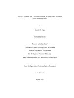
To have an overview of the historical importance of housing bubbles,
we repeat the same exercise for the 23 countries with available data from
the BIS residential price database.5 Figure 2.2 reports the evolution of
the fraction of countries in the sample with a housing bubble between
1980 and 2015. We want to remark two features of this figure. First,
housing bubble episodes are not rare events. In 52% of the quarters
5 The list of countries covered in the BIS residential property price is the following.
Australia, Belgium, Canada, Denmark, Finland, France, Germany, Hong Kong, Ireland,
Italy, Japan, Korea, Malaysia, Netherlands, New Zealand, Norway, South Africa, Spain,
Sweden, Switzerland, Thailand, UK and the USA.


2  A BRIEF HISTORY OF BUBBLES 

13

30

(% countries)

20

10

0
1980

1985


1990

1995

2000

2005

2010

2015

Fig. 2.2  World housing bubble indicator. Notes Bars indicate the percentage
of countries in the sample with the housing bubble indicator equal to one. The
bubble indicator is one if (i) the deviation of house prices from the trend is
higher than ½*standard deviation and (ii) nominal house prices are lower three
quarters later. House prices indices from BIS Residential Property Price database
( />
between 1980 and 2015, the bubble indicator was one for at least one
country in the sample. Second, the evolution of the world bubble indicator post-2000 seems different. Indeed, the housing bubble episodes in
the 2000s had a multi-country component that was not present before.
For instance, the peak of the world bubble indicator pre-2000 was June
1991–September 1992. It involved three countries, Switzerland, Japan
and Korea. In contrast, the largest peak in the sample occurred between
March 2008 and June 2008. In this case, the bubble indicator was one
for seven countries: Denmark, France, Ireland, Netherlands, South
Africa, Spain and UK. The housing bubble in the United States had collapsed two years before. Finally, it cannot be seen in the figure but the
size of the bubble (computed as the deviation of the house price index



14 

S. BASCO

from the linear trend) was also larger in the 2000s. Indeed, the average
bubble was almost three times larger in the bubble episodes of the late
2000s than during the 1990s (109 over 39).6 Therefore, it seems that
both the likelihood of having a global housing bubble and the size of
the bubble were increasing over time. These results are consistent with
the findings of Pavlidis et al. (2016), which use time-series techniques
to identify housing bubble episodes in a panel of 22 countries between
1975 and 2013. They also document an exceptional emergence and synchronization of housing bubble episodes in the late 2000s.7 In the next
chapters, we will offer a possible explanation for this increasing trend.

References
Brunnermeier, M. K. (2009). Bubbles. In L. Blume & S. Durlauf (Eds.), New
Palgrave Dictionary of Economics. Basingstoke: Palgrave Macmillan.
Giglio, S., Maggiori, M., & Stroebel, J. (2016). No-Bubble Condition: ModelFree Tests in Housing Markets. Econometrica, 84, 1047–1091.
Jordà, Ò., Schularick, M., & Taylor, A. M. (2015). Leveraged Bubbles. Journal
of Monetary Economics, 76, S1–S20.
Kindleberger, C. P., & Aliber, R. (2005). Manias, Panics, and Crashes: A History
of Financial Crises (5th ed.). Hoboken: Wiley. ISBN 0-471-46714-6.
Knoll, K., Schularick, M., & Steger, T. (2017). No Price Like Home: Global
House Prices, 1870–2012. American Economic Review, 107(2), 331–353.

6 The size of the bubble is computed as a simple average of the deviation from the trend
for the countries with the housing bubble indicator equal to one.
7 Other economists have attempted to identify housing bubbles. In an important
empirical contribution, Giglio et al. (2016) analyze the housing boom in London in the

late 2000s. As we will see in the next chapter, classical rational bubbles can only emerge
in infinite time horizon models. The authors take advantage of a peculiar feature of the
London housing market to compare the price of an “identical” house under two types of
ownership: (i) leaseholds (ownership expires in finite time, often more than 700 years) and
(ii) freeholds (there is no expiration date). Thus, theoretically, rational bubbles could only
emerge in houses under freehold ownership. Since they do not find a statistically significant
difference between the prices of houses under the two types of ownership, they conclude
that rational bubbles alone cannot explain the recent housing boom in London. The first
thing to remark is that the authors do not rule out the presence of a housing bubble in
London. Moreover, although they perform a very interesting exercise, we do not think that
their findings rule out rational bubbles as drivers of housing booms. In other words, as we
describe in the rest of the book, features of both rational and irrational bubbles seem relevant to describe the recent housing booms.


2  A BRIEF HISTORY OF BUBBLES 

15

Mackay, C. (1841). Memoirs of Extraordinary Popular Delusions and the Madness
of Crowds. London: Richard Bentley.
Pavlidis, E., Yusupova, A., Paya, I., Peel, D., Martínez-García, E., Mack, A.,
et al. (2016). Episodes of Exuberance in Housing Markets: In Search of the
Smoking Gun. Journal of Real Estate Finance and Economics, 53, 419–444.
Shiller, R. J. (2003). From Efficient Markets Theory to Behavioral Finance.
Journal of Economic Perspectives, 17(1), 83–104.
Temin, P., & Voth, H.-J. (2004). Riding the South Sea Bubble. American
Economic Review, 94(5), 1654–1668.


CHAPTER 3


Origin of Asset Price Bubbles

Abstract  The recurrence of asset price bubbles throughout ­
history
has stimulated the interest of economists in different generations.
We divide theories on the origin of bubbles in two: (i) behavioral and
(ii) rational. First, we explain how differences in the beliefs of agents may
result in bubbles (behavioral explanation). Second, we discuss how asset
price bubbles may emerge because the economy has a shortage of assets
(rational explanation). Finally, we develop a simple model to explain
how rational housing bubbles may appear in financially underdeveloped
economies.
Keywords  Behavioral
Financial constraint

· Rational bubbles · Shortage of assets ·

Asset price bubbles have triggered the interest of distinguished economists across generations. This list includes several Nobel Prize winners.
Starting with the late Paul Samuelson, who was awarded in the second edition (1970) and ending with the most recent Nobel Prize winner, Richard Thaler (2017). In between, Robert Shiller (2013) and
Jean Tirole (2014) have also been awarded with the Nobel Prize. This
(incomplete) list of economists help us to distinguish between two
very different views on the origin of asset price bubble episodes. The
first group, which includes Samuelson and Tirole, developed models
to explain how asset price bubbles can be the rational market response
© The Author(s) 2018
S. Basco, Housing Bubbles,
/>
17