Option pricing models (2007)
Bạn đang xem bản rút gọn của tài liệu. Xem và tải ngay bản đầy đủ của tài liệu tại đây (14.53 MB, 458 trang )
Option Pricing Models
and Volatility Using
Excel -VBA
FABRICE DOUGLAS ROUAH
GREGORY VAINBERG
John Wiley & Sons, Inc.
Option Pricing Models
and Volatility Using
Excel -VBA
Founded in 1807, John Wiley & Sons is the oldest independent publishing company
in the United States. With offices in North America, Europe, Australia, and Asia,
Wiley is globally committed to developing and marketing print and electronic
products and services for our customers’ professional and personal knowledge and
understanding.
The Wiley Finance series contains books written specifically for finance and
investment professionals as well as sophisticated individual investors and their
financial advisors. Book topics range from portfolio management to e-commerce,
risk management, financial engineering, valuation, and financial instrument analysis,
as well as much more.
For a list of available titles, visit our Web site at www.WileyFinance.com.
Option Pricing Models
and Volatility Using
Excel -VBA
FABRICE DOUGLAS ROUAH
GREGORY VAINBERG
John Wiley & Sons, Inc.
Copyright c 2007 by Fabrice Douglas Rouah and Gregory Vainberg. All rights reserved.
Published by John Wiley & Sons, Inc., Hoboken, New Jersey.
Published simultaneously in Canada.
Wiley Bicentennial Logo: Richard J. Pacifico
No part of this publication may be reproduced, stored in a retrieval system, or transmitted in any form
or by any means, electronic, mechanical, photocopying, recording, scanning, or otherwise, except as
permitted under Section 107 or 108 of the 1976 United States Copyright Act, without either the prior
written permission of the Publisher, or authorization through payment of the appropriate per-copy fee to
the Copyright Clearance Center, Inc., 222 Rosewood Drive, Danvers, MA 01923, (978) 750-8400, fax
(978) 750-4470, or on the Web at www.copyright.com. Requests to the Publisher for permission should
be addressed to the Permissions Department, John Wiley & Sons, Inc., 111 River Street, Hoboken, NJ
07030, (201) 748-6011, fax (201) 748-6008, or online at />Limit of Liability/Disclaimer of Warranty: While the publisher and author have used their best efforts in
preparing this book, they make no representations or warranties with respect to the accuracy or
completeness of the contents of this book and specifically disclaim any implied warranties of
merchantability or fitness for a particular purpose. No warranty may be created or extended by sales
representatives or written sales materials. The advice and strategies contained herein may not be suitable
for your situation. You should consult with a professional where appropriate. Neither the publisher nor
author shall be liable for any loss of profit or any other commercial damages, including but not limited
to special, incidental, consequential, or other damages.
For general information on our other products and services or for technical support, please contact our
Customer Care Department within the United States at (800) 762-2974, outside the United States at
(317) 572-3993 or fax (317) 572-4002.
Wiley also publishes its books in a variety of electronic formats. Some content that appears in print may
not be available in electronic books. For more information about Wiley products, visit our Web site at
www.wiley.com.
Designations used by companies to distinguish their products are often claimed as trademarks. In all
instances where John Wiley & Sons, Inc. is aware of a claim, the product names appear in initial capital
or all capital letters. Readers, however, should contact the appropriate companies for more complete
information regarding trademarks and registration.
Library of Congress Cataloging-in-Publication Data:
Rouah, Fabrice, 1964Option pricing models and volatility using Excel-VBA / Fabrice Douglas Rouah, Gregory Vainberg.
p. cm. –(Wiley finance series)
Includes bibliographical references and index.
ISBN: 978-0-471-79464-6 (paper/cd-rom)
1. Options (Finance)–Prices. 2. Capital investments–Mathematical–Mathematical models.
3. Options (Finance)–Mathematical models. 4. Microsoft Excel (Computer file) 5. Microsoft
Visual Basic for applications. I. Vainberg, Gregory, 1978-II. Title.
HG6024.A3R678 2007
332.64’53–dc22
2006031250
Printed in the United States of America.
10 9 8 7 6 5 4 3 2 1
To Jacqueline, Jean, and Gilles
—Fabrice
To Irina, Bryanne, and Stephannie
—Greg
Contents
Preface
ix
CHAPTER 1
Mathematical Preliminaries
1
CHAPTER 2
Numerical Integration
39
CHAPTER 3
Tree-Based Methods
70
CHAPTER 4
The Black-Scholes, Practitioner Black-Scholes, and Gram-Charlier Models
112
CHAPTER 5
The Heston (1993) Stochastic Volatility Model
136
CHAPTER 6
The Heston and Nandi (2000) GARCH Model
163
CHAPTER 7
The Greeks
187
CHAPTER 8
Exotic Options
230
CHAPTER 9
Parameter Estimation
275
vii
viii
CONTENTS
CHAPTER 10
Implied Volatility
304
CHAPTER 11
Model-Free Implied Volatility
322
CHAPTER 12
Model-Free Higher Moments
350
CHAPTER 13
Volatility Returns
374
APPENDIX A
A VBA Primer
404
References
409
About the CD-ROM
413
About the Authors
417
Index
419
Preface
his book constitutes a guide for implementing advanced option pricing models
and volatility in Excel/VBA. It can be used by MBA students specializing in
finance and risk management, by practitioners, and by undergraduate students in
their final year. Emphasis has been placed on implementing the models in VBA,
rather than on the theoretical developments underlying the models. We have made
every effort to explain the models and their coding in VBA as simply as possible.
Every model covered in this book includes one or more VBA functions that can be
accessed on the CD-ROM. We have focused our attention on equity options, and
we have chosen not to include interest rate options. The particularities of interest
rate options place them in a separate class of derivatives.
The first part of the book covers mathematical preliminaries that are used
throughout the book. In Chapter 1 we explain complex numbers and how to
implement them in VBA. We also explain how to write VBA functions for finding
roots of functions, the Nelder-Mead algorithm for finding the minimum of a
multivariate function, and cubic spline interpolation. All of these methods are used
extensively throughout the book. Chapter 2 covers numerical integration. Many of
option pricing and volatility models require that an integral be evaluated for which
no closed-form solution exists, which requires a numerical approximation to the
integral. In Chapter 2 we present various methods that have proven to be extremely
accurate and efficient for numerical integration.
The second part of this book covers option pricing formulas. In Chapter 3
we cover lattice methods. These include the well-known binomial and trinomial
trees, but also refinements such as the implied binomial and trinomial trees, the
flexible binomial tree, the Leisen-Reimer tree, the Edgeworth binomial tree, and
the adapted mesh method. Most of these methods approximate the Black-Scholes
model in discrete time. One advantage they have over the Black-Scholes model,
however, is that they can be used to price American options. In Chapter 4 we
cover the Black-Scholes, Gram-Charlier, and Practitioner Black-Scholes models, and
introduce implied volatility. The Black-Scholes model is presented as a platform
upon which other models are built. The Gram-Charlier model is an extension
of the Black-Scholes model that allows for skewness and excess kurtosis in the
distribution of the return on the underlying asset. The Practitioner Black-Scholes
model uses implied volatility fitted from a deterministic volatility function (DVF)
regression, as an input to the Black-Scholes model. It can be thought of as an
ad hoc method that adapts the Black-Scholes model to account for the volatility
smile in option prices. In Chapter 5 we cover the Heston (1993) model, which is
an extension of the Black-Scholes model that allows for stochastic volatility, while
T
ix
x
PREFACE
in Chapter 6 we cover the Heston and Nandi (2000) GARCH model, which in its
simplest form is a discrete-time version of the model in Chapter 5. The call price
in each model is available in closed form, up to a complex integral that must be
evaluated numerically. In Chapter 6 we also show how to identify the correlation
and dependence in asset returns, which the GARCH model attempts to incorporate.
We also show how to implement the GARCH(1,1) model in VBA, and how GARCH
volatilities can be used for long-run volatility forecasting and for constructing the
term structure of volatility. Chapter 7 covers the option sensitivities, or Greeks,
from the option pricing models covered in this book. The Greeks for the BlackScholes and Gram-Charlier models are available in closed form. The Greeks from
Heston (1993), and Heston and Nandi (2000) models are available in closed form
also, but require a numerical approximation to a complex integral. The Greeks
from tree-based methods can be approximated from option and asset prices at the
beginning nodes of the tree. In Chapter 7 we also show how to use finite differences
to approximate the Greeks, and we show that these approximations are all close to
their closed-form values. In Chapter 8 we cover exotic options. Most of the methods
we present for valuing exotic options are tree-based. Particular emphasis is placed
on single-barrier options, and the various methods that have been proposed to
deal with the difficulties that arise when tree-based methods are adapted to barrier
options. In Chapter 8 we also cover Asian options, floating-strike lookback options,
and digital options. Finally, in Chapter 9 we cover basic estimation methods for
parameters that are used as inputs to the option pricing models covered in this
book. Particular emphasis is placed on loss function estimation, which estimates
parameters by minimizing the difference between market and model prices.
The third part of this book deals with volatility and higher moments. In
Chapter 10 we present a thorough treatment of implied volatility and show how
the root-finding methods covered in Chapter 1 can be used to obtain implied
volatilities from market prices. We explain how the implied volatility curve can shed
information on the distribution of the underlying asset return, and we show how
option prices generated from the Heston (1993) and Gram-Charlier models lead
to implied volatility curves that account for the smile and skew in option prices.
Chapter 11 deals with model-free implied volatility. Unlike Black-Scholes implied
volatility, model-free implied volatility does not require the restrictive assumption
of a particular parametric form for the underlying price dynamics. Moreover, unlike
Black-Scholes implied volatilities, which are usually computed using at-the-money
or near-the-money options only, model-free volatilities are computed using the
whole cross-section of option prices. In Chapter 11 we also present methods that
mitigate the discretization and truncation bias brought on by using market prices
that do not include a continuum of strike prices, and that are available only over a
bounded interval of strike prices. We also show how to construct the Chicago Board
Options Exchange volatility index, the VIX, which is now based on model-free
implied volatility. Chapter 12 extends the model-free methods of Chapter 11, and
deals with model-free skewness and kurtosis. We show how applying interpolationextrapolation to these methods leads to much more accurate approximations to
xi
Preface
the integrals that are used to estimate model-free higher moments. In Chapter 13
we treat volatility returns, which are returns on strategies designed to profit from
volatility. We cover simple straddles, which are constructed using a single call and
put. Zero-beta straddles are slightly more complex, but have the advantage that they
are hedged against market movements. We also introduce a simple model to value
straddle options, and introduce delta-hedged gains. Similar to zero-beta straddles,
delta-hedged gains are portfolios in which all risks except volatility risk have been
hedged away, so that the only remaining risk to the portfolio is volatility risk.
Finally, we cover variance swaps, which are an application of model-free volatility
for constructing a call option on volatility.
This book also contains a CD-ROM that contains Excel spreadsheets and VBA
functions to implement all of the option pricing and volatility models presented in
this book. The CD-ROM also includes solutions to all the chapter exercises, and
option data for IBM Corporation and Intel Corporation downloaded from Yahoo!
(finance.yahoo.com).
ACKNOWLEDGMENTS
We have several people to thank for their valuable help and comments during the
course of writing this book. We thank Peter Christoffersen, Susan Christoffersen,
and Kris Jacobs. We also thank Steven Figlewski, John Hull, Yue Kuen Kwok, Dai
Min, Mark Rubinstein, and our colleagues Vadim Di Pietro, Greg N. Gregoriou,
and especially Redouane El-Kamhi. Working with the staff at John Wiley & Sons
has been a pleasure. We extend special thanks to Bill Falloon, Emilie Herman, Laura
Walsh, and Todd Tedesco. We are indebted to Polina Ialamova at OptionMetrics.
We thank our families for their continual support and personal encouragement.
Finally, we thank Peter Christoffersen, Steven L. Heston, and Espen Gaarder, for
kindly providing the endorsements.
CHAPTER
1
Mathematical Preliminaries
INTRODUCTION
In this chapter we introduce some of the mathematical concepts that will be needed to
deal with the option pricing and stochastic volatility models introduced in this book,
and to help readers implement these concepts as functions and routines in VBA.
First, we introduce complex numbers, which are needed to evaluate characteristic
functions of distributions driving option prices. These are required to evaluate the
option pricing models of Heston (1993) and Heston and Nandi (2000) covered in
Chapters 5 and 6, respectively. Next, we review and implement Newton’s method
and the bisection method, two popular and simple algorithms for finding zeros of
functions. These methods are needed to find volatility implied from option prices,
which we introduce in Chapter 4 and deal with in Chapter 10. We show how to
implement multiple linear regression with ordinary least squares (OLS) and weighted
least squares (WLS) in VBA. These methods are needed to obtain the deterministic
volatility functions of Chapter 4. Next, we show how to find maximum likelihood
estimators, which are needed to estimate the parameters that are used in option
pricing models. We also implement the Nelder-Mead algorithm, which is used to find
the minimum values of multivariate functions and which will be used throughout
this book. Finally, we implement cubic splines in VBA. Cubic splines will be used
to obtain model-free implied volatility in Chapter 11, and model-free skewness and
kurtosis in Chapter 12.
COMPLEX NUMBERS
Most of the numbers we are used to dealing with in our everyday lives are real
numbers, which are defined as any number lying on the real line = (−∞, +∞).
As such, real numbers can be positive or negative; rational, meaning that they can
be expressed as a fraction; or irrational, meaning that√they cannot be expressed as a
numbers,
fraction. Some examples of real numbers are 1/3, −3, 2, and π . Complex
√
however, are constructed around the imaginary unit i defined as i = −1. While i is
not a real number, i2 is a real number since i2 = −1. A complex number is defined as
1
2
OPTION PRICING MODELS AND VOLATILITY USING EXCEL-VBA
a = x + iy, where x and y are both real numbers, called the real and imaginary parts
of a, respectively. The notation Re[] and Im[] is used to denote these quantities, so
that Re[a] = x and Im[a] = y.
Operations on Complex Numbers
Many of the operations on complex numbers are done by isolating the real and
imaginary parts. Other operations require simple tricks, such as rewriting the
complex number in a different form or using its complex conjugate. Krantz (1999)
is a good reference for this section.
Addition and subtraction of complex numbers is performed by separate operation on the real and imaginary parts. It requires adding and subtracting, respectively,
the real and imaginary parts of the two complex numbers:
(x + iy) + (u + iv) = (x + u) + i(y + v),
(x + iy) − (u + iv) = (x − u) + i(y − v).
Multiplying two complex numbers is done by applying the distributive axiom to the
product, and regrouping the real and imaginary parts:
(x + iy)(u + iv) = (xu − yv) + i(xv + yu).
The complex conjugate of a complex number is defined as a = x − iy and is useful
for dividing complex numbers. Since aa = x2 + y2 , we can express division of any
two complex numbers as the ratio
(x + iy)(u − iv)
(xu + yv) + i(yu − xv)
x + iy
=
=
.
u + iv
(u + iv)(u − iv)
u2 + v2
Exponentiation of a complex number is done by applying Euler’s formula, which
produces
exp(x + iy) = exp(x) exp(iy) = exp(x)[cos(y) + i sin(y)].
Hence, the real part of the resulting complex number is exp(x) cos(y), and the
imaginary part is exp(x) sin(y). Obtaining the logarithm of a complex number
requires algebra. Suppose that w = a + ib and that its logarithm is the complex
number z = x + iy, so that z = log(w). Since w = exp(z), we know that a = ex cos(y)
the identity cos(y)2 + sin(y)2 =
and b = ex sin(y). Squaring these numbers, applying
√
2
1, and solving for x produces x = Re[z] = log( a + b2 ). Taking their ratio produces
b/a = sin(y)/cos(y) = tan(y),
and solving for y produces y = Im[z] = arctan(b/a).
3
Mathematical Preliminaries
It is now easy to obtain the square root of the complex number w = a + ib,
using DeMoivre’s Theorem:
[cos(x) + i sin(x)]n = cos(nx) + i sin(nx).
(1.1)
By arguments in the previous paragraph,
we can write w = r cos(y) + ir sin(y) = reiy ,
√
2
2
where y = arctan(b/a) and r = a + b . The square root of w is therefore
√
r[cos(y) + i sin(y)]1/2 .
Applying DeMoivre’s Theorem with n = 1/2, this becomes
√
r[cos( 2y ) + i sin( 2y )],
√
√
√
so that the real and imaginary parts of w are r cos( 2y ) and r sin( 2y ), respectively.
Finally, other functions of complex numbers are available, but we have not
included VBA code for these functions. For example, the cosine of a complex number z = x + iy produces another complex number, with real and imaginary parts
given by cos(x) cosh(y) and − sin(x) sinh(y) respectively, while the sine of a complex
number has real and imaginary parts sin(x) cosh(y) and − cos(x) sinh(y), respectively.
The hyperbolic functions cosh(y) and sinh(y) are defined in Exercise 1.1.
Operations Using VBA
In this section we describe how to define complex numbers in VBA and how to
construct functions for operations on complex numbers. Note that it is possible
to use the built-in complex number functions in Excel directly, without having to
construct them in VBA. However, we will see in later chapters that using the built-in
functions increases substantially the computation time required for convergence of
option prices. Constructing complex numbers in VBA, therefore, makes computation
of option prices more efficient. Moreover, it is sometimes preferable to have control
over how certain operations on complex numbers are defined. There are other
definitions of the square root of a complex number, for example, than that given by
applying DeMoivre’s Theorem. Finally, learning how to construct complex numbers
in VBA is a good learning exercise.
The Excel file Chapter1Complex contains VBA functions to define complex
numbers and to perform operations on complex numbers. Each function returns
the real part and the imaginary part of the resulting complex number. The first
step is to construct a complex number in terms of its two parts. The function
Set cNum() defines a complex number with real and imaginary parts given by
set cNum.rp and set cNum.ip, respectively.
Function Set_cNum(rPart, iPart) As cNum
Set_cNum.rP = rPart
Set_cNum.iP = iPart
End Function
4
OPTION PRICING MODELS AND VOLATILITY USING EXCEL-VBA
The function cNumProd() multiplies two complex numbers cNum1 and cNum2, and
returns the complex number cNumProd with real and imaginary parts cNumProd.rp
and cNumProd.ip, respectively.
Function cNumProd(cNum1 As cNum, cNum2 As cNum) As cNum
cNumProd.rP = (cNum1.rP * cNum2.rP) - (cNum1.iP * cNum2.iP)
cNumProd.iP = (cNum1.rP * cNum2.iP) + (cNum1.iP * cNum2.rP)
End Function
Similarly, the functions cNumDiv(), cNumAdd(), and cNumSub() return the
real and imaginary parts of a complex number obtained by, respectively, division,
addition, and subtraction of two complex numbers, while the function cNumConj() returns the conjugate of a complex number.
The function cNumSqrt() returns the square root of a complex number:
Function cNumSqrt(cNum1 As cNum) As cNum
r = Sqr(cNum1.rP ^ 2 + cNum1.iP ^ 2)
y = Atn(cNum1.iP / cNum1.rP)
cNumSqrt.rP = Sqr(r) * Cos(y / 2)
cNumSqrt.iP = Sqr(r) * Sin(y / 2)
End Function
The functions cNumExp() and cNumLn() produce, respectively, the exponential
of a complex number and the natural logarithm of a complex number using the VBA
function Atn() for the inverse tan function (arctan).
Function cNumExp(cNum1 As cNum) As cNum
cNumExp.rP = Exp(cNum1.rP) * Cos(cNum1.iP)
cNumExp.iP = Exp(cNum1.rP) * Sin(cNum1.iP)
End Function
Function cNumLn(cNum1 As cNum) As cNum
r = (cNum1.rP^2 + cNum1.iP^2)^0.5
theta = Atn(cNum1.iP / cNum1.rP)
cNumLn.rP = Application.Ln(r)
cNumLn.iP = theta
End Function
Finally, the functions cNumReal() and cNumIm() return the real and imaginary
parts of a complex number, respectively.
The Excel file Chapter1Complex illustrates how these functions work. The VBA
function Complexop2() performs operations on two complex numbers:
Function Complexop2(rP1, iP1, rP2, iP2, operation)
Dim cNum1 As cNum, cNum2 As cNum, cNum3 As cNum
Dim output(2) As Double
cNum1 = setcnum(rP1, iP1)
cNum2 = setcnum(rP2, iP2)
Select Case operation
Case 1: cNum3 = cNumAdd(cNum1, cNum2) ' Addition
5
Mathematical Preliminaries
Case 2: cNum3 = cNumSub(cNum1, cNum2) ' Subtraction
Case 3: cNum3 = cNumProd(cNum1, cNum2) ' Multiplication
Case 4: cNum3 = cNumDiv(cNum1, cNum2) ' Division
End Select
output(1) = cNum3.rP
output(2) = cNum3.iP
complexop2 = output
End Function
The Complexop2() function requires five inputs, a real and imaginary part for
each number, and the parameter corresponding to the operation being performed
(1 through 4). Its output is an array of dimension two, containing the real and
imaginary parts of the complex number. Figure 1.1 illustrates how this function
works. To add the two numbers 11 + 3i and −3 + 4i, which appear in ranges C4:D4
and C5:D5 respectively, in cell C6 we type
= Complexop2(C4,D4,C5,D5,F6)
and copy to cell D6, which produces the complex number 8 + 7i. Note that the
output of the Complexop2() function is an array. The appendix to this book explains
in detail how to output arrays from functions. Note also that the last argument
of the function Complexop2() is cell F6, which contains the operation number (1)
corresponding to addition.
FIGURE 1.1 Operations on Complex Numbers
6
OPTION PRICING MODELS AND VOLATILITY USING EXCEL-VBA
Similarly, the function Complexop1() performs operations on a single complex
number, in this example 4 + 5i. To obtain the complex conjugate, in cell C15
we type
= Complexop2(C14,D14,F15)
and copy to cell D15 This is illustrated in the bottom part of Figure 1.1.
Relevance of Complex Numbers
Complex numbers are abstract entities, but they are extremely useful because they
can be used in algebraic calculations to produce solutions that are tangible. In
particular, the option pricing models covered in this book require a probability
density function for the logarithm of the stock price, X = log(S). From a theoretical
standpoint, however, it is often easier to obtain the characteristic function ϕX (t) for
log(S), given by
ϕX (t) =
∞
eitx fX (x) dx,
0
where
√
i = −1,
fX (x) = probability density function of X.
The probability density function for the logarithm of the stock price can then be
obtained by inversion of ϕX (t):
fX (x) =
1
2π
∞
−∞
e−itx ϕX (t) dt
One corollary of Levy’s inversion formula—an alternate inversion formula—is that
the cumulative density function FX (x) = Pr(X < x) for the logarithm of the stock
price can be obtained. The following expression is often used for the risk-neutral
probability that a call option lies in-the-money:
FX (k) = Pr[log(S) > k] =
1
1
+
2 π
∞
Re
0
e−itk ϕX (t)
dt,
it
where k = log(K) is the logarithm of the√strike price K. Again, this formula requires
evaluating an integral that contains i = −1.
Mathematical Preliminaries
7
FINDING ROOTS OF FUNCTIONS
In this section we present two algorithms for finding roots of functions, the NewtonRaphson method, and the bisection method. These will become important in later
chapters that deal with Black-Scholes implied volatility. Since the Black-Scholes
formula cannot be inverted to yield the volatility, finding implied volatility must
be done numerically. For a given market price on an option, implied volatility is
that volatility which, when plugged into the Black-Scholes formula, produces the
same price as the market. Equivalently, implied volatility is that which produces a
zero difference between the market price and the Black-Scholes price. Hence, finding
implied volatility is essentially a root-finding problem.
The chief advantage of programming root-finding algorithms in VBA, rather
than using the Goal Seek and Solver features included in Excel, is that a particular
algorithm can be programmed for the problem at hand. For example, we will see
in later chapters that the bisection algorithm is particularly well suited for finding
implied volatility. There are at least four considerations that must be kept in mind
when implementing root-finding algorithms. First, adequate starting values must
be carefully chosen. This is particularly important in regions of highly functional
variability and when there are multiple roots and local minima. If the function is
highly variable, a starting value that is not close enough to the root might stray the
algorithm away from a root. If there are multiple roots, the algorithm may yield
only one root and not identify the others. If there are local minima, the algorithm
may get stuck in a local minimum. In that case, it would yield the minimum as
the best approximation to the root, without realizing that the true root lies outside
the region of the minimum. Second, the tolerance must be specified. The tolerance
is the difference between successive approximations to the root. In regions where
the function is flat, a high number for tolerance can be used. In regions where the
function is very steep, however, a very small number must be used for tolerance.
This is because even small deviations from the true root can produce values for the
function that are substantially different from zero. Third, the maximum number of
iterations needs to be defined. If the number of iterations is too low, the algorithm
may stop before the tolerance level is satisfied. If the number of iterations is too
high and the algorithm is not converging to a root because of an inaccurate starting
value, the algorithm may continue needlessly and waste computing time.
To summarize, while the built-in modules such as the Excel Solver or Goal Seek
allows the user to specify starting values, tolerance, maximum number of iterations,
and constraints, writing VBA functions to perform root finding sometimes allows
flexibility that built-in modules do not. Furthermore, programming multivariate
optimization algorithms in VBA, such as the Nelder-Mead covered later in this
chapter, is easier if one is already familiar with programming single-variable algorithms. The root-finding methods outlined in this section can be found in Burden
and Faires (2001) or Press et al. (2002).
8
OPTION PRICING MODELS AND VOLATILITY USING EXCEL-VBA
Newton-Raphson Method
This method is one of the oldest and most popular methods for finding roots of
functions. It is based on a first-order Taylor series approximation about the root.
To find a root x of a function f (x), defined as that x which produces f (x) = 0, select
a starting value x0 as the initial guess to the root, and update the guess using the
formula
f (xi )
f (xi+1 ) = xi −
(1.2)
f (xi )
for i = 0, 1, 2, . . ., and where f (xi ) denotes the first derivative of f (x) evaluated at
xi . There are two methods to specify a stopping condition for this algorithm, when
the difference between two successive approximations is less than the tolerance level
ε, or when the slope of the function is sufficiently close to zero. The VBA code in
this chapter uses the second condition, but the code can easily be adapted for the
first condition.
The Excel file Chapter1Roots contains the VBA functions for implementing the
root-finding algorithms presented in this section. The file contains two functions
for implementing the Newton-Raphson method. The first function assumes that an
analytic form for the derivative f (xi ) exists, while the second uses an approximation
to the derivative. Both are illustrated with the simple function f (x) = x2 − 7x + 10,
which has the derivative f (x) = 2x − 7. These are defined as the VBA functions
Fun1() and dFun1(), respectively.
Function Fun1(x)
Fun1 = x^2 - 7*x + 10
End Function
Function dFun1(x)
dFun1 = 2*x - 7
End Function
The function NewtRap() assumes that the derivative has an analytic form, so
it uses the function Fun1() and its derivative dFun1() to find the root of Fun1. It
requires as inputs the function, its derivative, and a starting value x guess. The
maximum number of iterations is set at 500, and the tolerance is set at 0.00001.
Function NewtRap(fname As String, dfname As String, x_guess)
Maxiter = 500
Eps = 0.00001
cur_x = x_guess
For i = 1 To Maxiter
fx = Run(fname, cur_x)
dx = Run(dfname, cur_x)
If (Abs(dx) < Eps) Then Exit For
cur_x = cur_x - (fx / dx)
Next i
NewtRap = cur_x
End Function
9
Mathematical Preliminaries
The function NewRapNum() does not require the derivative to be specified, only
the function Fun1() and a starting value. At each step, it calculates an approximation
to the derivative.
Function NewtRapNum(fname As String, x_guess)
Maxiter = 500
Eps = 0.000001
delta_x = 0.000000001
cur_x = x_guess
For i = 1 To Maxiter
fx = Run(fname, cur_x)
fx_delta_x = Run(fname, cur_x - delta_x)
dx = (fx - fx_delta_x) / delta_x
If (Abs(dx) < Eps) Then Exit For
cur_x = cur_x - (fx / dx)
Next i
NewtRapNum = cur_x
End Function
The function NewtRapNum() approximates the derivative at any point x by
using the line segment joining the function at x and at x + dx, where dx is a small
number set at 1×10⁻⁹ . This is the familiar ‘‘rise over run’’ approximation to the
slope, based on a first-order Taylor series expansion for f (x + dx) about x:
f (x) ≈
f (x) − f (x + dx)
.
dx
This approximation appears as the statement
dx = (fx - fx_delta_x) / delta_x
in the function NewtRapNum().
Bisection Method
This method is well suited to problems for which the function is continuous on an
interval [a, b] and for which the function is known to take a positive value on one
endpoint and a negative value on the other endpoint. By the Intermediate Value
Theorem, the interval will necessarily contain a root. A first guess for the root is the
midpoint of the interval. The bisection algorithm proceeds by repeatedly dividing
the subintervals of [a, b] in two, and at each step locating the half that contains the
root. The function BisMet() requires as inputs the function for which a root must
be found, and the endpoints a and b. The endpoints must be chosen so that the
function assumes opposite signs at each, otherwise the algorithm may not converge.
Function BisMet(fname As String, a, b)
Eps = 0.000001
If (Run(fname, b) < Run(fname, a)) Then
10
OPTION PRICING MODELS AND VOLATILITY USING EXCEL-VBA
tmp = b: b = a: a = tmp
End If
Do While (Run(fname, b) - Run(fname, a) > Eps)
midPt = (b + a) / 2
If Run(fname, midPt) < 0 Then
a = midPt
Else
b = midPt
End If
Loop
BisMet = (b + a) / 2
End Function
We will see in Chapters 4 and 10 that the bisection method is particularly well
suited for finding implied volatilities extracted from option prices.
Illustration of the Methods
Figure 1.2 illustrates the Newton-Raphson method with an explicit derivative, the
Newton-Raphson method with an approximation to the derivative, and the Bisection
method. This spreadsheet appears in the Excel file Chapter1Roots. As before, we use
the function f (x) = x2 − 7x + 10, coded by the VBA function Fun1(), with derivative
f (x) = 2x − 7, coded by the VBA function dFun1(). It is easy to see by inspection
that this function has two roots, at x = 2 and at x = 5. We illustrate the methods
with the first root.
The bisection method requires an interval with endpoints chosen so that the
function takes on values opposite in sign at each endpoint. Hence, we choose the
FIGURE 1.2 Root-Finding Algorithms